P.A. Cucis | C. Berger-Vachon | R. Hermann | H. Thaï-Van | S. Gallego | E. Truy
OPEN ACCESS
The cochlear implant is the most successful implantable device for the rehabilitation of profound deafness. However, in some cases, the electrical stimulation delivered by the electrode can spread inside the cochlea creating overlap and interaction between frequency channels. By using channel-selection algorithms like the “nofm” coding-strategy, channel interaction can be reduced. This paper describes the preliminary results of experiments conducted with normal hearing subjects (n = 9). Using a vocoder, the present study simulated the hearing through a cochlear implant. Speech understanding in noise was measured by varying the number of selected channels (“nofm”: 4, 8, 12 and 16of20) and the degree of simulated channel interaction (“Low”, “Medium”, “High”). Also, with the vocoder, we evaluated the impact of simulated channel interaction on frequency selectivity by measuring psychoacoustic tuning curves. The results showed a significant average effect of the signal-to-noise ratio (p < 0.0001), the degree of channel interaction (p < 0.0001) and the number of selected channels, (p = 0.029). The highest degree of channel interaction significantly decreases intelligibility as well as frequency selectivity. These results underline the importance of measuring channel interaction for cochlear implanted patients to have a prognostic test and to adjust fitting methods in consequence. The next step of this project will be to transpose these experiments to implant users, to support our results.
cochlear implant, speech in noise, simulation, psychoacoustic tuning curves, channel interaction
There are different types of hearing aids, and the cochlear implant is one of them. It is a neuroprosthetic device that bypasses the sensory cells of the inner-ear and transforms acoustic information into electrical pulses received by the auditory system (Figure 1). It is primarily intended for severe and profound bilateral deafness. It can be used for children with congenital hearing loss or for adults that have lost their hearing through time [1]. Thanks to the technological improvements of the last decades, modern cochlear implants provide very good results in terms of hearing and quality of life [2, 3].
Cochlear implant signal processing follows the principles of the vocoder [4], this is why different types of vocoders are often used with normal-hearing subjects to simulate the performances of cochlear implanted patients [5-7]. The acoustic signal is divided into several frequency bands (the channels) and the variations of spectral energy over time are calculated. In some cochlear implant simulators, sounds are created by modulating narrowband noises containing the same frequencies as those selected for the input analysis [8]. In a real cochlear implant, the spectral energy of the channels is sent to the electrodes (one channel per electrode). Then, modulated electrical pulses activate the neurons of the inner-ear. Pitch is coded by the stimulation site: a basal stimulation of the cochlea is interpreted by the auditory system as a high-pitched sound, while an apical stimulation gives a low-pitched sensation. With multi-electrode implants, speech understanding is greatly improved; however, channel interaction is often cited as one of the reasons for poor performances.
The activation of the auditory neurons by the electrodes is not as accurate as the natural mechanical activation in normal-hearing people. The cochlear implant operates on a disabled auditory system with reduced nerve survival and nerve repartition [9]. Moreover, an electrode stimulates the area directly in front of it, but also common areas with the neighboring electrodes which can cause an overlap between the neuronal frequency channels. The overlap is more or less important depending on the amplitude of the electric field and its diffusion in the cochlear fluid. The spread of excitation combined with the overlapping stimulation is referred to as channel interaction. One of the solutions suggested by cochlear implant manufacturers is the “nofm” codding strategy (standing for “n out of m”). The “nofm” algorithms reduce the number of stimulating electrodes in each analysis time-frame by performing a channel selection. The algorithm only keeps the “maxima”: the “n” most energetic channels among the “m” available [10]. As the overall number of channels and the number of selected “maxima” increase the spectral information, there is also an increased risk of channel interaction [11-13]. Nevertheless, in noisy places, more channels are indicated to maintain an acceptable speech intelligibility [14].
Figure 1. Cochlear Implant. a) The external behind-the-ear processor receives, converts, and sends the auditory information to the internal part via a radio frequency antenna, b) The internal receiver decodes the information and activates the electrode array which stimulates the cochlea
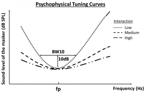
The number of “maxima” is usually subjectively defined in a quiet environment by the hearing care professional during a dialog with the patient. However, the optimal number of “maxima” is thought to be related to channel interaction [15]. It would therefore seem useful to take this into account during the fitting appointments. Indeed, some psychoacoustic measurements can account for channel interaction because overlapping stimulations can change the perceived loudness [16]. This principle is used to measure psychophysical tuning curves (PTC) whose “V-shape” reflects the frequency selectivity of the ear [17]. The level of masking required at a specific frequency thus gives an overview of the overlap degree. For a cochlear implant, each point on the PTC reflects the minimum intensity required for an electrode to mask the reference electrode (probe) [18, 19]. Channel interaction reduces frequency selectivity and flattens the PTC. A parameter called Q10 is used to characterize the curve frequency selectivity (Figure 2). The Q10 is the ratio between the probe frequency value (fp in Hertz) and the bandwidth taken 10 dB above the bottom of the curve (BW10 in Hertz) (1). The higher the Q10, the better the frequency selectivity.
Figure 2. Psychophysical tuning curves and the effect of channel interaction on frequency selectivity
$Q 10=f p / B W 10$ (1)
Currently, only a few studies assess Q10 in normal-hearing subjects using a vocoder that simulates channel interaction [20].
This paper introduces the first results of a study performed with normal-hearing subjects listening to a cochlear implant simulator. This experiment tested: 1) The effect of the number of “maxima” on word recognition in noise when combined with a simulation of channel interaction. 2) The impact of channel interaction on frequency selectivity.
2.1 Subjects
Nine native French speakers aged from 19 to 40 years old (Mean = 30.3 years) took part in this study. Pure tone audiometry was performed on all participants to verify that their hearing was normal (average hearing loss below 20 dB HL on each ear for 500, 1000, 2000, and 4000 Hz) The study was approved by the French ethics comity Est IV (April 12, 2019) and was supervised by the Civil Hospitals of Lyon.
2.2 Material
The subjects were tested in a soundproof room using TDH 39 audiometric headphones from Telephonics. The stimuli were generated by a standard laptop computer. An external M-Track MkII sound card from M-Audio was used for digital-to-analog conversion. Stimulation levels were calibrated by a Madsen Orbiter 922 clinical audiometer.
2.3 Protocol
The study took place at the ORL department of the Edouard Herriot Hospital in Lyon and each appointment lasted approximately 4 hours. A session consisted of the following steps:
2.4 Vocoder signal processing
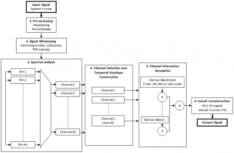
A 20-channel vocoder was used to reproduce the signal processing of a Neurelec/Oticon Medical© cochlear implant. Such as a real cochlear implant, speech and noise were summed at the required signal to noise ratio (SNR) before being processed by the vocoder. The signal processing sequence is depicted in Figure 3.
The signal processing performed by the vocoder followed six main steps:
Figure 3. Synoptic diagram of the signal processing performed by the vocoder used in the study
Table 1. Cutoff frequencies of the vocoder, number of bins distributed per channel
|
Channel Number |
20 |
19 |
18 |
17 |
16 |
15 |
14 |
13 |
12 |
11 |
|
Lower Cutoff (Hz) |
195 |
326 |
456 |
586 |
716 |
846 |
977 |
1107 |
1237 |
1367 |
|
Higher Cutoff (Hz) |
326 |
456 |
586 |
716 |
846 |
977 |
1107 |
1237 |
1367 |
1497 |
|
Filter bandwidth (Hz) |
131 |
130 |
130 |
130 |
130 |
131 |
130 |
130 |
130 |
130 |
|
Bin (s) per channel |
1 |
1 |
1 |
1 |
1 |
1 |
1 |
1 |
1 |
1 |
|
|
|
|
|
|
|
|
|
|
|
|
|
Channel Number |
10 |
9 |
8 |
7 |
6 |
5 |
4 |
3 |
2 |
1 |
|
Lower Cutoff (Hz) |
1497 |
1758 |
2018 |
2409 |
2799 |
3451 |
4102 |
4883 |
5794 |
6836 |
|
Higher Cutoff (Hz) |
1758 |
2018 |
2409 |
2799 |
3451 |
4102 |
4883 |
5794 |
6836 |
8008 |
|
Filter bandwidth (Hz) |
261 |
260 |
391 |
390 |
652 |
651 |
781 |
911 |
1042 |
1172 |
|
Bin (s) per channel |
2 |
2 |
3 |
3 |
5 |
5 |
6 |
7 |
8 |
9 |
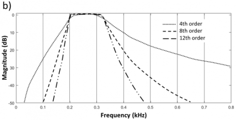
Figure 4. Vocoder output and sound reconstruction in the vocoder, a) filtering, modulation, and summation; b) Bode diagrams: 4th, 8th, and 12th order Butterworth filters
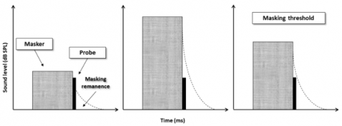
Figure 5. Schematic representation of the forward masking paradigm
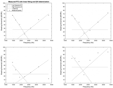
Figure 6. Examples of linear fitting used to evaluate the frequency selectivity of psychophysical tuning curves
2.5 Speech audiometry in noise
Subjects were instructed to repeat each word after it was presented to them. Words were extracted from Fournier's dissyllabic lists (e.g. “le bouchon” = “the cork”) and mixed with a “Cocktail-Party” noise (a mixture of chatter and tableware noises). The lists were calibrated to 65 dB SPL by a clinical audiometer and played through headphones to the subject's right ear. Each list consisted of 10 words, and the unit of error was the syllable, giving a final score between 0 and 20. Word lists were processed by the vocoder. A combination of the three parameters was attributed to each list: noise level, degree of overlap, and number of maxima. All in all, there were 36 possible conditions, i.e. 36 different lists out of the 40 existing ones.
2.6 Psychophysical tuning curves
Thanks to a program coded with MATLAB, the stimuli were generated and presented to the right ear. To find the masking threshold, the sound levels were adapted according to the answers given by the subject. A tuning curve was established for each level of simulated interaction for a probe frequency of fp = 2226 Hz corresponding to channel number 8 of the Digisonic SP (Neurelec©). The masking sounds correspond to channels 11 to 5, i.e. fm = 1440.5, 1637, 1898.5, 2226, 2619, 3143, and 3798 Hz respectively. The measurement followed a forward masking paradigm (sequential) (Figure 5). A 110-ms masker was followed by a 20-ms probe with no time delay between them. For each listener, a hearing threshold and a maximum acceptable level were measured for the maskers and the probe.
We used an adaptive three intervals forced-choice (3IFC) method [21], to measure the masking thresholds. The level adaptation followed a “2Up-1Down” paradigm, the sound level of the masker was increased by one step when the subject identified the probe sound twice in a row and decreased by one step when the subject made a mistake. There was a 4 dB step for the first three reversals, decreased to 2 dB for reversals three to six, and 1 dB for the last six. There were 12 reversals inside a run and the masked threshold was defined, in dB SPL, as the average masker level at the last six reversals.
2.7 Tuning curves fitting and Q10
A program has been developed to calculate the Q10 from a data table containing the measured masking thresholds. Slopes on both sides were considered monotonic, so if a masked threshold did not follow this rule with a deviation higher than 10 dB, it was not taken into account for the regression. The typical fitted-function included all the seven masking thresholds except for 2 subjects: subject S04 (6 points for the “Low” curve and 5 points for the “Medium” curve) and S07 (6 points, “Medium” curve). Figure 6 shows some examples of the results obtained with the fitting algorithm.
3.1 Speech audiometry in noise
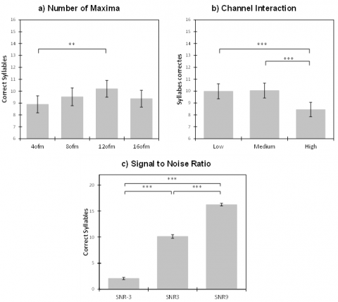
The repeated measure ANOVA, based on a linear mixed model, showed a significant effect of the simulated channel interaction, the number of maxima and the SNR with p < 0.0001, p = 0.029, and p < 0.0001 respectively. The interaction effects were not significant. The results are shown in Figure 7. T-tests were used for post-hoc testing. For the number of maxima, the significance level was α = 0.05/6 = 0.008 according to the Bonferroni correction. For the simulated channel interaction, α = 0.05/3 = 0.016. First, we observe that with 12 maxima the average intelligibility was 10.2 syllables (out of 20 syllables); it was significantly different from the intelligibility of 8.9 syllables observed with 4 maxima (p = 0.006). Then, there were significant differences between the average syllable recognition for the “High” interaction (8.44 syllables) and the syllable recognition (9.98 and 10.05 syllables respectively) for the “Low” and “Medium” interaction, p < 0.0001. Finally, the RSB gave for the three noise levels, significant differences, p < 0.0001 (respectively 2.1; 10.1 and 16.2 out of 20).
Figure 7. Results of the 3-way repeated measures ANOVA and the Wilcoxon tests. (A) Average syllable recognition across the number of maxima, (B) across the levels of channel interaction, (C) across the signal-to-noise ratios. Error bars represent ±1 standard error of the mean
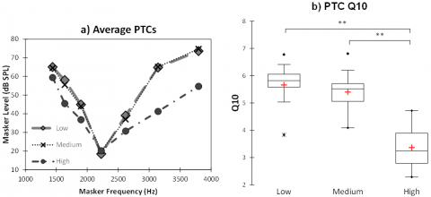
Figure 8. Comparison of the sharpness (Q10) of the average psychophysical tuning curves (PTC) function of the degree of channel interaction. (A) Average tuning curves for the three levels of excitation spread. (B) Boxplots showing Q10dB: the horizontal line within the box indicates the median; means are indicated by a plus sign; edges are the 25th and 75th percentiles
3.2 Psychophysical tuning curves
The Friedman test, revealed a significant effect of the degree of inter-channel overlap on the Q10 (p = 0.001). Then, the pair-wise comparisons (Wilcoxon tests) showed that the average Q10 for the “High” degree of interaction was significantly lower than the average Q10 for the “Low” and “Medium” interaction (3.37, 5.66 and 5.40). “Low” - “Medium” p = 0.426; “Low” - “High” p = 0.004; “Medium” - “High” p = 0.004 (Bonferroni, α = 0.017) (Figure 8).
In this study, we measured word recognition in noise and frequency selectivity with normal-hearing subjects using a cochlear implant simulation. Thanks to the simulator, several degrees of channel interaction and different number of maxima were tested. The results presented here are prelaminar and correspond to the measurements performed with 9 subjects.
The results showed a significant average effect of the number of selected maxima and a significant effect of the degree of simulated channel interaction on word recognition in noise.
Regarding the number of maxima, there was a significant improvement of intelligibility from 4 to 12 maxima, however, there is no significant change from 8 to 12 and from 12 to 16. The plateau effect seen between 8 and 16 is consistent with the literature on the number of channels [13] and in particular with the study by Dorman et al. who observed an intelligibility plateau at 9 maxima and no improvement from 9 to 20 [14].
About the effect of simulated channel interaction, the “High” level (-24 dB/oct filter) significantly reduced word recognition compared to the “Low” and “Medium” levels that gave similar results (-48 and -72 dB/oct). It seems therefore necessary to exceed a certain amount of interaction to impair speech understanding. Similar results can be found in the literature, for example in the experiment of Jahn et al. the recognition of consonants and vowels was significantly reduced by simulating a “High” interaction (-15 dB/oct filter) compared to the results obtained with lower interaction (-30 and -60 dB/oct) [15]. The small difference of performance observed between “Low” and “Medium” interaction could be explained by the proximity of shape between the filters (Figure 4b). The difference could be insufficient to create a difference in intelligibility. There is a ratio of 1.5 between the slopes of the “Low” and “Medium” filters (72 on 48 dB/oct), whereas if we compare them with the “High” filter, the ratios are 2 and 3 (48 on 24 dB/oct and 72 on 24 dB/oct).
Finally, it should be noted that the statistical interaction effects considering the relationship between the three variables were not significant. It may indicate that the effects of channel interaction, number of maxima, and signal to noise ratio on word recognition are independent of each other. This result seems surprising because one might think that intelligibility increases with the number of maxima. Therefore, it would be better to confirm that point, first with a larger number of normal-hearing subjects, but also in a real situation with cochlear implant users.
The frequency selectivity was also significantly changed by the level of channel interaction. The results showed that the “High” interaction leads to a significantly lower frequency selectivity reflected by a lower Q10. Measuring frequency selectivity through a vocoder is not very common in the literature. Only the article by Langner et al. shows a change in Q10 in simulation by varying the frequency selectivity of the vocoder [20]. Thus, this result confirms the relationship between the Q10 value and channel interaction.
To conclude, our simulation study highlighted a plateau effect of the number of maxima on word recognition and showed that, on average, there is a maximum recognition with 12 maxima out of 20. Moreover, changing channel interaction led to a similar profile in both experiments (word recognition in noise and frequency selectivity) and impaired perceptions only at the highest simulated level (Figures 6 and 7b). These preliminary results follow the data in the literature but they have to be completed: first, with more normal-hearing subjects and further statistical analyses, and secondly, by performing an equivalent study with cochlear implant users.
The authors would like to thank the people and institutions that allowed to carry out this work: the subjects who participated in the experiments and the entire staff of the ORL and Audiology Department at Edouard Herriot University Hospital, Civil Hospitals of Lyon. We also thank Dan Gnansia, Pierre Stahl, and the company Neurelec/Oticon Medical, for the support provided to the entire project.
[1] Clark, G., Richter, C.P. (2004). Cochlear implants: Fundamentals and applications. Physics Today, 57(11): 66-67. https://doi.org/10.1063/1.1839383
[2] Dhanasingh, A., Jolly, C. (2017). An overview of cochlear implant electrode array designs. Hearing Research, 356: 93-103. https://doi.org/10.1016/j.heares.2017.10.005
[3] McRackan, T.R., Bauschard, M., Hatch, J.L., Franko-Tobin, E., Droghini, H.R., Nguyen, S.A., Dubno, J.R. (2018). Meta-analysis of quality-of-life improvement after cochlear implantation and associations with speech recognition abilities. The Laryngoscope, 128(4): 982-990. https://doi.org/10.1002/lary.26738
[4] Loizou, P.C. (2006). Speech processing in vocoder-centric cochlear implants. Cochlear and Brainstem Implants, 64: 109-143. https://doi.org/10.1159/000094648
[5] Karoui, C., James, C., Barone, P., Bakhos, D., Marx, M., Macherey, O. (2019). Searching for the sound of a cochlear implant: Evaluation of different vocoder parameters by cochlear implant users with single-sided deafness. Trends in hearing, 23: 2331216519866029. https://doi.org/10.1177/2331216519866029
[6] Seldran, F., Thai-Van, H., Truy, E., Berger-Vachon, C., Collet, L., Gallego, S., Beliaeff, M. (2010). Simulation of an EAS implant with a hybrid vocoder. Cochlear Implants International, 11(sup1): 125-129. https://doi.org/10.1179/146701010X12671177544302
[7] Shannon, R.V., Zeng, F.G., Kamath, V., Wygonski, J., Ekelid, M. (1995). Speech recognition with primarily temporal cues. Science, 270(5234): 303-304. https://doi.org/10.1126/science.270.5234.303
[8] Griffin, D.W., Lim, J.S. (1988). Multiband excitation vocoder. IEEE Transactions on Acoustics, Speech, and Signal Processing, 36(8): 1223-1235. https://doi.org/10.1109/29.1651
[9] Shannon, R.V. (1983). Multichannel electrical stimulation of the auditory nerve in man. II. Channel interaction. Hearing Research, 12(1): 1-16. https://doi.org/10.1016/0378-5955(83)90115-6
[10] Wilson, B.S., Dorman, M.F. (2008). Cochlear implants: a remarkable past and a brilliant future. Hearing Research, 242(1-2): 3-21. https://doi.org/10.1016/j.heares.2008.06.005
[11] Berger-Vachon, C., Djedou, B., Collet, L., Morgon, A. (1992). Model for understanding the influence of some parameters in cochlear implantation, pp. 42-45. https://doi.org/10.1177/000348949210100112
[12] Faulkner, A., Rosen, S., Wilkinson, L. (2001). Effects of the number of channels and speech-to-noise ratio on rate of connected discourse tracking through a simulated cochlear implant speech processor. Ear and Hearing, 22(5): 431-438. https://doi.org/10.1097/00003446-200110000-00007
[13] Shannon, R.V., Fu, Q.J., Galvin Iii, J. (2004). The number of spectral channels required for speech recognition depends on the difficulty of the listening situation. Acta Oto-Laryngologica, 124(0): 50-54. https://doi.org/10.1080/03655230410017562
[14] Dorman, M.F., Loizou, P.C., Spahr, A.J., Maloff, E. (2002). A comparison of the speech understanding provided by acoustic models of fixed-channel and channel-picking signal processors for cochlear implants. J. Speech Lang. Hear. Res., 45(4): 783-788. https://doi.org/10.1044/1092-4388(2002/063)
[15] Jahn, K.N., DiNino, M., Arenberg, J.G. (2019). Reducing simulated channel interaction reveals differences in phoneme identification between children and adults with normal hearing. Ear and Hearing, 40(2): 295-311. https://doi.org/10.1097/AUD.0000000000000615
[16] Tang, Q., Benítez, R., Zeng, F.G. (2011). Spatial channel interactions in cochlear implants. Journal of Neural Engineering, 8(4): 046029. https://doi.org/10.1088/1741-2560/8/4/046029
[17] Moore, B.C. (1978). Psychophysical tuning curves measured in simultaneous and forward masking. The Journal of the Acoustical Society of America, 63(2): 524-532. https://doi.org/10.1121/1.381752
[18] Nelson, D.A., Kreft, H.A., Anderson, E.S., Donaldson, G.S. (2011). Spatial tuning curves from apical, middle, and basal electrodes in cochlear implant users. The Journal of the Acoustical Society of America, 129(6): 3916-3933. https://doi.org/10.1121/1.3583503
[19] Nelson, D.A., Donaldson, G.S., Kreft, H. (2008). Forward-masked spatial tuning curves in cochlear implant users. The Journal of the Acoustical Society of America, 123(3): 1522-1543. https://doi.org/10.1121/1.2836786
[20] Langner, F., Jürgens, T. (2016). Forward-masked frequency selectivity improvements in simulated and actual cochlear implant users using a preprocessing algorithm. Trends in Hearing, 20: 2331216516659632. https://doi.org/10.1177/2331216516659632
[21] Levitt, H.C.C.H. (1971). Transformed up-down methods in psychoacoustics. The Journal of the Acoustical Society of America, 49(2B): 467-477. https://doi.org/10.1121/1.1912375