M.A. Gazi | P.P. Gharami | R. Biswas | S.F. Ahmmed*
OPEN ACCESS
An exploration has been perpetrated to study the heat and mass transfer flow of an incompressible electrically conducting Maxwell fluid past a stretching sheet in the presence of nanoparticle with Soret and Dufour effects. The governing partial differential equations are transformed into dimensionless momentum, energy and concentration equations and are solved numerically by using explicit finite difference method (EFDM) by employing Compact visual FORTRAN 6.6a programming algorithm. For optimizing the system parameter and accuracy of the system the stability and convergence analysis was carried out. It was observed that with the initial boundary conditions, for ∆τ=0.0005, ∆X=0.67, ∆Y=0.167, the system converged at prandtl number Pr≥0.044 and Schmidt number Sc≥0.036.The dominance of various physical parameters on the flow, heat and mass translation characteristics are speculated through diagram and tables.
Maxwell fluid, Explicit Finite Difference Method (EFDM), stretching sheet, nanoparticles
Now a day the research sector of engineering and industry is being attracted by the flow disposition of non-Newtonian fluids because of its upbeat applications. The evocation of polymers fluids, animal bloods, solidification of melted crystals, exotic lubricants is important. A non-linear relationship between the stress and rate of strain has been perpetrated by various fluids such as shampoo, polymer solutions and paints. Maxwell model is one of the subclass of rate type fluids. This model retrenches the complicating payoff of shear-dependent viscosity from any boundary layer exploration and qualifies, one to concentrate exclusively on the outcome of fluids pliability on the nature which is seen in the boundary layer Sakiadis et al. [1]. Some polymeric solutions, glycerin etc. are such kinds of fluids. An analytic solution for unsteady MHD flow in a rotating Maxwell fluid through a porous medium was developed by Hayat et al. [2]. Tan and Mustafa [3] discussed linear convective stability of a Maxwell fluid layer in a porous medium. Some recent investigators (Abel et al. [4]; Kamran et al. [5]; Abbas et al. [6] and Hayat et al. [7]) dealt with the flows of Maxwell fluids.
The analysis of heat transfer of MHD Maxwell fluid flow past a stretching sheet in the presence of thermal radiation effect can be perfectly significant. The impact of thermal radiation on MHD flow of a Maxwell fluid over a stretching sheet was discussed by Aliakbar et al. [8]. Zargartelebi et al. [9] has discussed the heat transfer of Nano fluids towards stretching sheet in the stagnation point. The heat transfer in a Maxwell fluid over an oscillating vertical plate has studied by Khan et al. [10]. Satya Narayana et al. [11] have dissolved the effects of thermal radiation and heat source on MHD nanofluid past a vertical plate in a rotating system. MHD boundary layer flow of a Maxwell fluid past a stretching sheet in the presence of nanoparticles was viewed by Nadeem et al. [12]. Samir Kumar Nandy [13] has studied an unsteady flow of Maxwell fluid in the presence of nanoparticles toward a permeable shrinking surface with Navier slip. Many researchers (Biswas et al. [14-17]; Hayat et al. [18]) have studied the problem of Maxwell fluid flow over a stretching sheet analytically and numerically under different geometries.
The efflux of Maxwell fluid on MHD heat and mass metastasis problems with chemical reaction is of illustrious practical appreciation in much affiliation of science and engineering. The action, such as absorbing, volatilization at the periphery of a water corpse, and the efflux in a plain cooler etc needs to be considered. Unsteady flow of a Maxwell fluid over a stretching surface in presence of chemical reaction is commenced by Mukhopadhyay and Rama Subba Reddy [19]. Satya Narayana et al. [20] inspected the Hall current and chemical reaction effects on MHD micropolar fluid in a rotating frame of reference. Satya Narayana et al. [21] presented Chemical reaction and Radiation absorption effects on MHD micropolar fluid past a vertical porous plate in a rotating system. Noor [22] analyzed the flow behavior of a Maxwell fluid in the presence of thermophoresis and chemical reaction. Vertical stretching sheet is considered in this investigation. Mukhopadhyay and Bishnoi et al. [23] have performed their exploration work to look into the effect of chemical reaction on some mass transfer related Maxwell fluid flow problems. Also, this type of work is done by Biswas et al. [24-27]; Ahmmed, et al. [28, 29] and Mondal et al. [30].
Heat and mass transfer ascend simultaneously between the flow and the leading potentials are of more fabricated in nature. Dufour or diffusion-thermo effect is resulted from the energy flux and the energy fluxes are caused by a composition gradient. Soret or thermal-diffusion effect is involved with mass fluxes which are also related with the temperature gradient. Bishnoi and Bilal [31] have presented three Dimensional Flow of Maxwell Fluid with Soret and Dufour Effects. Venkateswarlu and Satya Narayana [32] investigated the influence of variable thermal conductivity on MHD Casson fluid flow over a stretching sheet with viscous dissipation, Soret and Dufour effects. Recently Venkateswarlu and Satya Narayana [20] viewed soret and dufour effects on MHD flow over a stretching sheet with joule heating.
The Maxwell fluid flow, heat and mass transfer past a stretching surface with Dufour and Soret effects in the presence of nanoparticles is discussed here is a fundamental one that arises in many practical situations such as polymer extrusion process. Keeping this in view, the main objective of the present work is the numerical investigation of thermo diffusion and diffusion thermo effects over a stretching sheet with heat source and viscous dissipation. Similarity solutions are obtained and the reduced ordinary differential equations are solved numerically using explicit finite difference scheme. The effects of different flow parameters encountered in the equations are studied with the help of their graphical representations and tables.
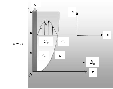
We consider the two dimensional steady mixed convective heat and mass transfer of viscous incompressible boundary layer flow of a Maxwell fluid past a stretching sheet. The -axis is considered in the direction along the sheet and the -axis is normal to the surface. The flow is generated due to the stretching of sheet by applying two equal and opposite forces along the x-axis. A uniform transverse magnetic field of strength B0 is imposed along the y-axis and the chemical reaction is taking place in the flow. We also proposed that the plate is maintained at variable temperature and concentration, Tw(x)>T∞ and Cw(x)>C∞ respectively, where T∞ is the uniform temperature of the ambient fluid and C∞ is the uniform ambient concentration.
Figure 1. Physical configuration and co-ordinate system
Under the usual boundary layer approximation, the governing equations are:
$\frac{\partial u}{\partial x}+\frac{\partial v}{\partial y}=0$ (1)
$\frac{\partial u}{\partial t}+u\frac{\partial u}{\partial x}+v\frac{\partial u}{\partial y}=\upsilon \frac{{{\partial }^{2}}u}{\partial {{y}^{2}}}-{{\lambda }_{1}}\left( {{u}^{2}}\frac{{{\partial }^{2}}u}{\partial {{x}^{2}}}+{{v}^{2}}\frac{{{\partial }^{2}}u}{\partial {{y}^{2}}}+2uv\frac{{{\partial }^{2}}u}{\partial x\partial y} \right)+g{{\beta }_{T}}\left( T-{{T}_{\infty }} \right)+g{{\beta }_{C}}\left( C-{{C}_{\infty }} \right)-\frac{\sigma B_{0}^{2}}{\rho }$ (2)
$\frac{\partial T}{\partial t}+u\frac{\partial T}{\partial x}+v\frac{\partial T}{\partial y}=\alpha \frac{{{\partial }^{2}}T}{\partial {{y}^{2}}}+\tau \left[ {{D}_{B}}\frac{\partial T}{\partial y}\frac{\partial C}{\partial y}+\frac{{{D}_{T}}}{{{T}_{\infty }}}{{\left( \frac{\partial T}{\partial y} \right)}^{2}} \right]-\frac{1}{\rho {{c}_{p}}}\frac{\partial {{q}_{r}}}{\partial y}+\frac{{{D}_{m}}{{K}_{T}}}{{{C}_{S}}{{C}_{P}}}\frac{{{\partial }^{2}}C}{\partial {{y}^{2}}}+\frac{{{Q}_{0}}}{\rho {{c}_{p}}}\left( T-{{T}_{\infty }} \right)$ (3)
$\frac{\partial C}{\partial t}+u\frac{\partial C}{\partial x}+v\frac{\partial C}{\partial y}={{D}_{m}}\frac{{{\partial }^{2}}C}{\partial {{y}^{2}}}+\frac{{{D}_{m}}{{K}_{T}}}{{{T}_{m}}}\frac{{{\partial }^{2}}T}{\partial {{y}^{2}}}-{{K}_{c}}{{\left( C-{{C}_{\infty }} \right)}^{p}}$ (4)
The associate boundary conditions are
$\left. \begin{align} & t=0,\,\,\,u=cx,\,\,\,v=0,\,\,\,T={{T}_{\infty }},\,\,\,C={{C}_{\infty }}\,\,\,\,\,\text{everywhere} \\ & t=0,\,\,\,u=cx,\,\,\,v=0,\,\,\,T={{T}_{\infty }},\,\,\,C={{C}_{\infty }}\,\,\,\text{at}\,\,\,x=0 \\ & u=cx,\,\,\,v=0,\,\,\,T={{T}_{w}},\,\,\,C={{C}_{w}}\,\,\,\text{at}\,\,\,y=0 \\ & u=0,\,\,\,v=0,\,\,\,T\to {{T}_{\infty }},\,\,\,C\to {{C}_{\infty }}\,\,\,\text{as}\,\,\,y\to \infty \\ \end{align} \right\}$ (5)
Rosseland approximation is being used for the simplification of radiation heat flux as follows ${{q}_{r}}=-\frac{4{{\sigma }_{s}}}{3{{k}_{e}}}\frac{\partial {{T}^{4}}}{\partial y}$.
In the fluid flow if it is considered small temperature difference then qr is identified by elucidating T4 in Taylor series at T∞ and then insulting the higher order terms we get ${{T}^{4}}\cong 4{{T}_{\infty }}^{3}T-3{{T}_{\infty }}^{4}$. After that equation (3) becomes
$\frac{\partial T}{\partial t}+u\frac{\partial T}{\partial x}+v\frac{\partial T}{\partial y}=\alpha \frac{{{\partial }^{2}}T}{\partial {{y}^{2}}}+\tau \left[ {{D}_{B}}\frac{\partial T}{\partial y}\frac{\partial C}{\partial y}+\frac{{{D}_{T}}}{{{T}_{\infty }}}{{\left( \frac{\partial T}{\partial y} \right)}^{2}} \right]+\frac{16{{\sigma }_{s}}{{T}_{\infty }}^{3}}{3{{k}_{e}}\rho {{c}_{p}}}\frac{{{\partial }^{2}}T}{\partial {{y}^{2}}}+\frac{{{D}_{m}}{{K}_{T}}}{{{C}_{S}}{{C}_{P}}}\frac{{{\partial }^{2}}C}{\partial {{y}^{2}}}+\frac{{{Q}_{0}}}{\rho {{c}_{p}}}\left( T-{{T}_{\infty }} \right)$ (6)
For solving the equation (1-6) dimensionless segments are considered as
$X=\frac{x{{U}_{0}}}{\upsilon },\,\,\,Y=\frac{y{{U}_{0}}}{\upsilon },\,\,\,U=\frac{u}{{{U}_{0}}},\,\,\tau =\frac{t{{U}_{0}}}{\upsilon },\,\,\,\theta =\frac{T-{{T}_{\infty }}}{{{T}_{w}}-{{T}_{\infty }}},\,\,\,\phi =\frac{C-{{C}_{\infty }}}{{{C}_{w}}-{{C}_{\infty }}}$ (7)
Now the dimensionless form of the governing equations
$\frac{\partial U}{\partial X}+\frac{\partial V}{\partial Y}=0$ (8)
$\frac{\partial U}{\partial \tau }+U\frac{\partial U}{\partial X}+V\frac{\partial V}{\partial Y}=\frac{{{\partial }^{2}}U}{\partial {{Y}^{2}}}+Gr\theta +Gm\phi -Nv\left[ {{U}^{2}}\frac{{{\partial }^{2}}U}{\partial {{X}^{2}}}+{{V}^{2}}\frac{{{\partial }^{2}}U}{\partial {{Y}^{2}}}+2UV\frac{{{\partial }^{2}}U}{\partial X\partial Y} \right]-MU$ (9)
$\frac{\partial \theta }{\partial \tau }+U\frac{\partial \theta }{\partial X}+V\frac{\partial \theta }{\partial Y}=\frac{1}{\Pr }\left( 1+\frac{16R}{3} \right)\frac{{{\partial }^{2}}\theta }{\partial {{Y}^{2}}}+Nb\frac{\partial \theta }{\partial Y}\frac{\partial \phi }{\partial Y}+Nt{{\left( \frac{\partial \theta }{\partial Y} \right)}^{2}}+Du{{\left( \frac{\partial \phi }{\partial Y} \right)}^{2}}+Q\theta $ (10)
$\frac{\partial \phi }{\partial \tau }+U\frac{\partial \phi }{\partial X}+V\frac{\partial \phi }{\partial Y}=\frac{1}{Sc}\frac{{{\partial }^{2}}\phi }{\partial {{Y}^{2}}}+Sr\frac{{{\partial }^{2}}\theta }{\partial {{Y}^{2}}}-Kr{{C}^{p}}$ (11)
Also the corresponding boundary conditions
$\left. \begin{align} & \tau \le 0,\,\,\,U=0,\,\,\,V=0,\,\,\,\theta =0,\,\,\,\phi =0\,\,\,\,\,\text{everywhere} \\ & \tau >0,\,\,\,U=0,\,\,\,V=0,\,\,\,\theta =0,\,\,\,\phi =0\,\,\,\,\text{at}\,\,X=0 \\ & U=cX=c,\,\,\,V=0,\,\,\,\theta =1,\,\,\,\phi =1\,\,\,\,\,\,\,\text{at}\,\,Y=0 \\ & U=0,\,\,\,V=0,\,\,\,\theta =0,\,\,\,\phi =0\,\,\,\text{as}\,\,Y\to \infty \\ \end{align} \right\}$ (12)
The non dimensionless quantities which is represent the skin friction, the Nusselt number and Sherwood number is as follows:
${{C}_{f}}=-\frac{1}{2\sqrt{2}}G{{r}^{-\frac{3}{4}}}{{\left( \frac{\partial U}{\partial Y} \right)}_{Y=0}}$ (13)
${{N}_{u}}=\frac{1}{\sqrt{2}}G{{r}^{-\frac{3}{4}}}{{\left( \frac{\partial \theta }{\partial Y} \right)}_{Y=0}}$ (14)
${{S}_{h}}=\frac{1}{\sqrt{2}}G{{r}^{-\frac{3}{4}}}{{\left( \frac{\partial \phi }{\partial Y} \right)}_{Y=0}}$ (15)
The continuity equation which is satisfied by stream function $\psi \left( X,Y \right)$ and is amalgamated with the velocity components in the usual way as
$U=\frac{\partial \psi}{\partial Y}, V=-\frac{\partial \psi}{\partial X}$
To solve the governing coupled non-dimensional partial differential equations with the associated initial and boundary conditions. It is considered that the plate of height Xmax(=125) i.e. X varies from 0 to 125 and regard Ymax(=125) i.e. Y varies from 0 to 25. There are m=150 and n=300 grid spacing in the X and Y directions respectively as shown in Figure. 2. It is assumed that ∆X, ∆Y are constant mesh sizes along X and Y directions respectively and taken, ∆X=0.83 (0≤X≤125); ∆Y=0.83 (0≤Y≤125); with the smaller time interval ∆τ= 0.0005.
Figure 2. The finite difference space grid
With the help of explicit finite difference method equations:
$\frac{{{U}_{i,j}}-{{U}_{i-1,j}}}{\Delta X}+\frac{{{V}_{i,j}}-{{V}_{i-1,j}}}{\Delta Y}=0$ (16)
$\frac{U_{i, j}^{\prime}-U_{i, j}}{\Delta \tau}+U_{i, j} \frac{U_{i, j}-U_{i-1, j}}{\Delta X}+V_{i, j} \frac{U_{i, j+1}-U_{i, j}}{\Delta Y}=\frac{U_{i, j+1}-2 U_{i, j}+U_{i, j-1}}{(\Delta Y)^{2}}$ $+G r \theta_{i, j}+G m \phi_{i, j}-M U_{i, j}$
$-N v\left[\begin{array}{l}\left(U_{i, j}\right)^{2} \frac{U_{i, j+1}-2 U_{i, j}+U_{i, j-1}}{(\Delta X)^{2}}+\left(V_{i, j}\right)^{2} \frac{U_{i, j+1}-2 U_{i, j}+U_{i, j-1}}{(\Delta Y)^{2}} \\ +\left(2 U_{i, j} V_{i, j} \frac{U_{i+1, j+1}-U_{i+1, j-1}-U_{i-1, j+1}+U_{i-1, j-1}}{4 \Delta X \Delta Y}\right)\end{array}\right]$ (17)
$\begin{align} & \frac{{{\theta }^{'}}_{i,j}-{{\theta }_{i,j}}}{\Delta \tau }+{{U}_{i,j}}\frac{{{\theta }_{i,j}}-{{\theta }_{i-1,j}}}{\Delta X}+{{V}_{i,j}}\frac{{{\theta }_{i,j}}-{{\theta }_{i-1,j}}}{\Delta Y}=\frac{1}{\Pr }\left( 1+R \right)\frac{{{\theta }_{i,j+1}}-2{{\theta }_{i,j}}+{{\theta }_{i,j-1}}}{{{\left( \Delta Y \right)}^{2}}}+Q{{\theta }_{i,j}} \\ & +Du\frac{{{\phi }_{i,j+1}}-2{{\phi }_{i,j}}+{{\phi }_{i,j-1}}}{{{\left( \Delta Y \right)}^{2}}}+{{N}_{b}}\left( \frac{{{\theta }_{i,j+1}}-{{\theta }_{i,j}}}{\Delta Y}.\frac{{{\phi }_{i,j+1}}-{{\phi }_{i,j}}}{\Delta Y} \right)+{{N}_{t}}{{\left( \frac{{{\theta }_{i,j+1}}-{{\theta }_{i,j}}}{\Delta Y} \right)}^{2}} \\ \end{align}$ (18)
$\frac{{{\phi }^{'}}_{i,j}-{{\phi }_{i,j}}}{\Delta \tau }+{{U}_{i,j}}\frac{{{\phi }_{i,j}}-{{\phi }_{i-1,j}}}{\Delta X}+{{V}_{i,j}}\frac{{{\phi }_{i,j+1}}-{{\phi }_{i,j}}}{\Delta Y}=\frac{1}{Sc}\left( \frac{{{\phi }_{i,j+1}}-2{{\phi }_{i,j}}+{{\phi }_{i,j-1}}}{{{\left( \Delta Y \right)}^{2}}} \right)+Sr\left( \frac{{{\theta }_{i,j+1}}-2{{\theta }_{i,j}}+{{\theta }_{i,j-1}}}{{{\left( \Delta Y \right)}^{2}}} \right)-Kr{{\left( {{\phi }_{i,j}} \right)}^{p}}$ (19)
The associated boundary conditions become,
$\left. \begin{align} & U_{i,0}^{n}=1,\,\,\,\theta _{i,0}^{n}=1,\,\,\,\phi _{i,0}^{n}=1 \\ & U_{i,L}^{n}=0,\,\,\,\theta _{i,L}^{n}=0,\,\,\,\phi _{i,L}^{n}=0\,\,\,\text{where},L\to \infty \\ \end{align} \right\}$ (20)
Hither, i and j denotes the grid points with X and Y coordinates respectively and $\tau =n\Delta \tau $ where n=1,2,3…
For the constant mesh size the stability criteria of the scheme may be established as follows. The general term of the Fourier expansion for E, F and G at time τ is given below,
$\left. \begin{align} & E:E\left( \tau \right){{e}^{i\alpha x}}{{e}^{i\beta y}} \\ & F:F\left( \tau \right){{e}^{i\alpha x}}{{e}^{i\beta y}} \\ & G:G\left( \tau \right){{e}^{i\alpha x}}{{e}^{i\beta y}} \\ \end{align} \right\}$ (21)
After a time step these terms convert to
$\left. \begin{align} & E:{E}'\left( \tau \right){{e}^{i\alpha x}}{{e}^{i\beta y}} \\ & F:{F}'\left( \tau \right){{e}^{i\alpha x}}{{e}^{i\beta y}} \\ & G:{G}'\left( \tau \right){{e}^{i\alpha x}}{{e}^{i\beta y}} \\ \end{align} \right\}$ (22)
Substituting equation (21) and (22) to the equation (17-19) we get,
$\begin{align} & {E}'=E\left( \tau \right)+\Delta \tau [GrF+GmG-ME+\frac{\left( 2\cos \beta \Delta Y-1 \right)}{{{\left( \Delta Y \right)}^{2}}}E-\frac{U\left( 1-{{e}^{i\alpha \Delta X}} \right)}{\Delta X}E-\frac{V\left( {{e}^{i\beta \Delta Y}}-1 \right)}{\Delta Y} \\ & -Nv[\frac{2{{U}^{2}}E\left( 1-\cos \alpha \Delta X \right)}{{{\left( \Delta X \right)}^{2}}}+\frac{2{{V}^{2}}E\left( \cos \beta \Delta Y-1 \right)}{{{\left( \Delta Y \right)}^{2}}}+2EUV\frac{\left( {{e}^{i\alpha \left( X+\Delta X \right)}}{{e}^{i\beta \left( Y+\Delta Y \right)}}-{{e}^{i\alpha \left( X+\Delta X \right)}}{{e}^{i\beta \left( Y-\Delta Y \right)}} \right)}{4\Delta X\Delta Y} \\ & -2EUV\frac{\left( {{e}^{i\alpha \left( X-\Delta X \right)}}{{e}^{i\beta \left( Y+\Delta Y \right)}}-{{e}^{i\alpha \left( X-\Delta X \right)}}{{e}^{i\beta \left( Y-\Delta Y \right)}} \right)}{4\Delta X\Delta Y}]] \\\end{align}$
$\begin{align} & \Rightarrow {E}'=[1+\frac{2\left( \cos \beta \Delta Y-1 \right)}{{{\left( \Delta Y \right)}^{2}}}-\Delta \tau M-\frac{U\Delta \tau \left( 1-{{e}^{i\alpha \Delta X}} \right)}{\Delta X}-\frac{V\Delta \tau \left( {{e}^{i\beta \Delta Y}}-1 \right)}{\Delta Y} \\ & -Nv[\frac{2{{U}^{2}}\Delta \tau \left( 1-\cos \alpha \Delta X \right)}{{{\left( \Delta X \right)}^{2}}}+\frac{2{{V}^{2}}\Delta \tau \left( \cos \beta \Delta Y-1 \right)}{{{\left( \Delta Y \right)}^{2}}}+2\Delta \tau UV\frac{\left( {{e}^{i\alpha \left( X+\Delta X \right)}}{{e}^{i\beta \left( Y+\Delta Y \right)}}-{{e}^{i\alpha \left( X+\Delta X \right)}}{{e}^{i\beta \left( Y-\Delta Y \right)}} \right)}{4\Delta X\Delta Y} \\ & -2\Delta \tau UV\frac{\left( {{e}^{i\alpha \left( X-\Delta X \right)}}{{e}^{i\beta \left( Y+\Delta Y \right)}}-{{e}^{i\alpha \left( X-\Delta X \right)}}{{e}^{i\beta \left( Y-\Delta Y \right)}} \right)}{4\Delta X\Delta Y}]]E+\Delta \tau GrF+\Delta \tau GmG \\ \end{align}$
$\Rightarrow {E}'={{A}_{1}}E+{{A}_{2}}F+{{A}_{3}}G$ (23)
where,
$\begin{align} & {F}'=F+\Delta \left( \tau \right)[\frac{1}{\Pr }\left( 1+R \right)\frac{2F\left( \cos \beta \Delta Y-1 \right)}{{{\left( \Delta Y \right)}^{2}}}+QF-\frac{U\left( 1-{{e}^{i\alpha \Delta X}} \right)}{\Delta X}F-\frac{V\left( {{e}^{i\beta \Delta Y}}-1 \right)}{\Delta Y}E \\ & +NbFC{{\left\{ \frac{\left( {{e}^{i\beta \Delta Y}}-1 \right)}{\Delta Y} \right\}}^{2}}+Du\frac{2K\left( \cos \beta \Delta Y-1 \right)}{{{\left( \Delta Y \right)}^{2}}}+NtTF{{\left\{ \frac{\left( {{e}^{i\beta \Delta Y}}-1 \right)}{\Delta Y} \right\}}^{2}}] \\ \end{align}$
$\begin{align} & \Rightarrow {F}'=F\left[ 1+\Delta \left( \tau \right)\frac{1}{\Pr }\left( 1+R \right)\frac{2\left( \cos \beta \Delta Y-1 \right)}{{{\left( \Delta Y \right)}^{2}}}+Q\Delta \left( \tau \right)+NbC\Delta \left( \tau \right){{\left\{ \frac{\left( {{e}^{i\beta \Delta Y}}-1 \right)}{\Delta Y} \right\}}^{2}}+NtT\Delta \left( \tau \right){{\left\{ \frac{\left( {{e}^{i\beta \Delta Y}}-1 \right)}{\Delta Y} \right\}}^{2}} \right] \\ & +E\left[ -\frac{U\Delta \left( \tau \right)\left( 1-{{e}^{i\alpha \Delta X}} \right)}{\Delta X}-\frac{V\Delta \left( \tau \right)\left( {{e}^{i\beta \Delta Y}}-1 \right)}{\Delta Y} \right]+Du\frac{2\Delta \left( \tau \right)\left( \cos \beta \Delta Y-1 \right)}{{{\left( \Delta Y \right)}^{2}}}G \\\end{align}$
$\Rightarrow {F}'={{A}_{4}}F+{{A}_{5}}G$ (24)
where,
${{A}_{4}}=1+\Delta \left( \tau \right)\frac{1}{\Pr }\left( 1+R \right)\frac{2\left( \cos \beta \Delta Y-1 \right)}{{{\left( \Delta Y \right)}^{2}}}+Q\Delta \left( \tau \right)+NbC\Delta \left( \tau \right){{\left\{ \frac{\left( {{e}^{i\beta \Delta Y}}-1 \right)}{\Delta Y} \right\}}^{2}}+NtT\Delta \left( \tau \right){{\left\{ \frac{\left( {{e}^{i\beta \Delta Y}}-1 \right)}{\Delta Y} \right\}}^{2}}$
$\begin{align} & {G}'=G+\Delta \tau [\frac{1}{Sc}\frac{2\left( \cos \beta \Delta Y-1 \right)}{{{\left( \Delta Y \right)}^{2}}}G+Sr\frac{2\left( \cos \beta \Delta Y-1 \right)}{{{\left( \Delta Y \right)}^{2}}}F-Kr{{G}^{P}}-\frac{U\left( 1-{{e}^{i\alpha \Delta X}} \right)}{\Delta X}G-\frac{V\left( {{e}^{i\beta \Delta Y}}-1 \right)}{\Delta Y}G] \\ & \\ \end{align}$
$\Rightarrow {G}'=G[1+\Delta \tau \frac{1}{Sc}\frac{2\left( \cos \beta \Delta Y-1 \right)}{{{\left( \Delta Y \right)}^{2}}}-Kr\Delta \tau -\frac{U\Delta \tau \left( 1-{{e}^{i\alpha \Delta X}} \right)}{\Delta X}-\frac{V\Delta \tau \left( {{e}^{i\beta \Delta Y}}-1 \right)}{\Delta Y}]+Sr\frac{2\left( \cos \beta \Delta Y-1 \right)}{{{\left( \Delta Y \right)}^{2}}}F$
$\Rightarrow {G}'={{A}_{6}}G+{{A}_{7}}E$ (25)
where,
${{A}_{6}}=1+\Delta \tau \frac{1}{Sc}\frac{2\left( \cos \beta \Delta Y-1 \right)}{{{\left( \Delta Y \right)}^{2}}}-Kr\Delta \tau -\frac{U\Delta \tau \left( 1-{{e}^{i\alpha \Delta X}} \right)}{\Delta X}-\frac{V\Delta \tau \left( {{e}^{i\beta \Delta Y}}-1 \right)}{\Delta Y}$
and,
${{A}_{7}}=Sr\frac{2\left( \cos \beta \Delta Y-1 \right)}{{{\left( \Delta Y \right)}^{2}}}$
Equation (23-25) can be manifested by matrix form
$\left[ \begin{align} & {{E}'} \\ & {{F}'} \\ & {{G}'} \\ \end{align} \right]=\left[ \begin{matrix} {{A}_{1}} & {{A}_{2}} & {{A}_{3}} \\ 0 & {{A}_{4}} & {{A}_{5}} \\ 0 & {{A}_{7}} & {{A}_{6}} \\\end{matrix} \right]\left[ \begin{matrix} E \\ F \\ G \\\end{matrix} \right]\text{ }i.e.\text{ }{\eta }'={T}'\eta $
where,
${\eta }'=\left[ \begin{matrix} {{E}'} \\ {{F}'} \\ {{G}'} \\\end{matrix} \right]$; ${T}'=\left[ \begin{matrix} {{A}_{1}} & {{A}_{2}} & {{A}_{3}} \\ 0 & {{A}_{4}} & {{A}_{5}} \\ {{A}_{7}} & 0 & {{A}_{6}} \\\end{matrix} \right]$
and
$\eta =\left[ \begin{matrix} E \\ F \\ G \\\end{matrix} \right]$
Let $a_{1}=\Delta \tau, b_{1}=U \frac{\Delta \tau}{\Delta X}, c_{1}=|-V| \frac{\Delta \tau}{\Delta X}$ and $d_{1}=2 \frac{\Delta \tau}{(\Delta Y)^{2}}$. Here a1, b1, c1 and d1 are all real and positive number. So the extreme modulus of A1, A4 and A6 occurs when $\alpha \Delta X=m \pi$ and $\beta \Delta Y=n \pi$ where both m and n are odd integers. Therefore
$A_{4}=1-2\left[d_{1} \frac{1}{\operatorname{Pr}}(1+R)+\frac{a_{1}}{2} Q+b_{1}+c_{1}+2 N b C d_{1}+2 N t T d_{1}\right]$
$A_{6}=1-2\left[d_{1} \frac{1}{S c}+b_{1}+c_{1}+\frac{a_{1}}{2} K r\right]$
To satisfy the probable values are $A_{1}=-1, A_{4}=-1$ and $A_{6}=-1$. Under this discretion the stability conditions of the method are
$U \frac{\Delta \tau}{\Delta X}+V \frac{\Delta \tau}{\Delta X}+\frac{2}{\operatorname{Pr}}(1+R) \frac{\Delta \tau}{(\Delta Y)^{2}}-\frac{\Delta \tau Q}{2}+2 N b \frac{\Delta \tau}{(\Delta Y)^{2}}+2 N t \frac{\Delta \tau}{(\Delta Y)^{2}} \leq 1$
and,
$U\frac{\Delta \tau }{\Delta X}+V\frac{\Delta \tau }{\Delta X}+\frac{1}{Sc}\frac{2\Delta \tau }{{{\left( \Delta Y \right)}^{2}}}+\frac{\Delta \tau Kr}{2}\le 1$
For, $U=V=T=0, \Delta \tau=0.0005, \Delta Y=0.167$ and $\Delta X=0.67$ then existing problem will be converged at $\mathrm{Pr} \geq 0.044$ and $S c \geq 0.036$.
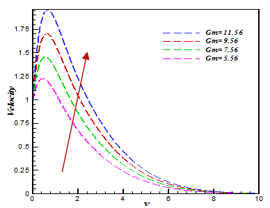
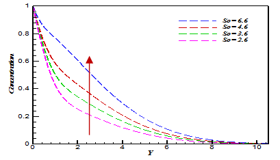
The numerical solutions are executed for velocity, temperature, concentration, the skin friction coefficient, the local Nusselt number, and the local Sherwood number for different values of occupying parameters. The numerical outcomes which are adopted for several values of different parameter are exhibited in the Figurers [1-24]. In order to attain the numerical inferences, the posterior values of default parameter are recherché as: $G m=5.56, G r=0.56, \operatorname{Pr}=0.20, R=0.20, Q=0.10, D u=0.20, N b=0.10, N t=0.40, K r=0.20, M=2.0$, $S c=2.60, N v=0.20, S o=2.60$.
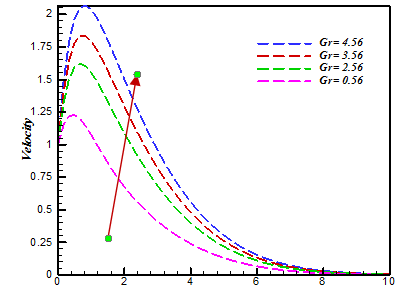
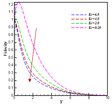
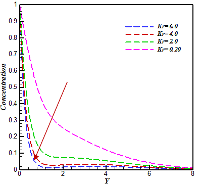
Figure 3 explain the impact of modified Grashof number (Gm) on the velocity profile. It is executed that with the increase of (Gm) parameter the velocity profile is increased. But, in Figure 4 velocity increases due to the increase of Grashof number (Gr), because the thermal Grashof number which signifies the relative effect of the thermal buoyancy force in the boundary layer. Figure 5 and Figure 6 respectively, show the velocity and concentration distributions for different values of the chemical reaction parameter Kr.
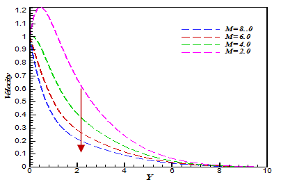
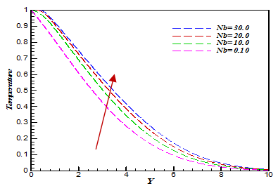
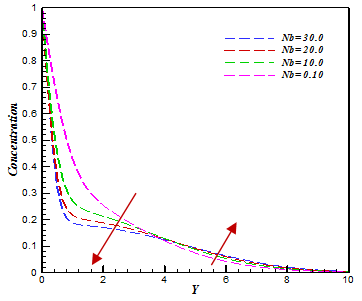
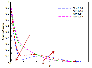
The velocity scheme for detached values of magnetic field parameter (M) is exhibited in Figure 7. It is clearly noticed that the velocity field extenuates with improvement of magnetic field parameter (M) towards the surface. In Figure 8 and Figure 9 elucidate the variations of temperature and concentration profiles for several values of Brownian parameter Nb. It is clearly seen that the improvement in the value of Nb≥0.10 the thermal boundary layer enhances and the concentration boundary layer reduces. The numerical value obtained from the EFDM simulation for Brownian parameter (Nb) varies from 0.10 to 30. Thermophoresis is the transport force that occurs due to the presence of a temperature gradient. From Figure 10 it can be observed that the concentration profile increases with the increase of thermophoresis parameter (Nt).
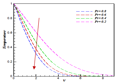
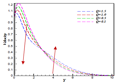
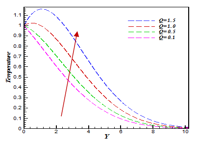
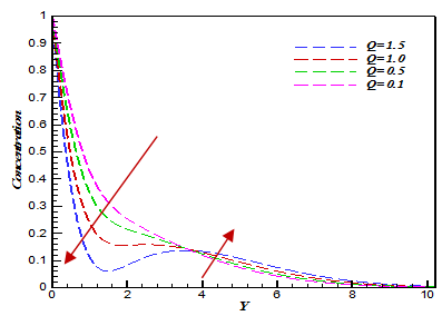
The parameter Pr is the proportion of kinematics viscosity to the thermal diffusivity. In Figure 11 represents that thermal boundary layer thickness downfall with the increase of Prandtl number. The effect of different values of Pr on temperature profiles is illustrated that the thermal boundary layer thickness increases with the decreasing values of Pr. Figure 12 is prepared to see the variation of the concentration profile. In the Figure 13, Figure 14 and Figure 15 is represented the effect of heat generation on the velocity, temperature and the concentration profile. The dimensionless Concentration distribution for different values of heat generation parameter Q is illustrated in Figure 15.
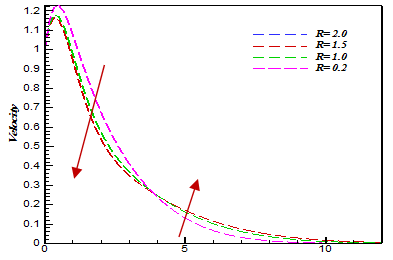
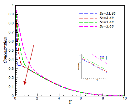
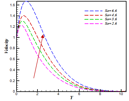
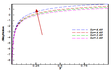
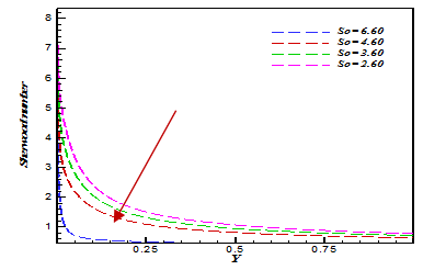
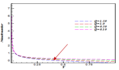
Figure 16 are graphical representation of the velocity profiles for different values of the thermal radiation parameter R. From Figure 17 it is noticed that, the indulgent motion of nanoparticles get decreased with an increase in Schmidt number (Sc). Figure 18 and Figure 19 respectively, show the velocity and concentration field for different values of Soret number (So). The impact of soret number (So) on skin friction and Sherwood number profile is given in Figure 20 and Figure 21. It is evident from this figure the value of Soret number (So) enhances by increasing skin friction whereas the reverse trend is observed for the Sherwood number. The impact of heat source (Q) on Nusselt number is shown on the Figure 22.
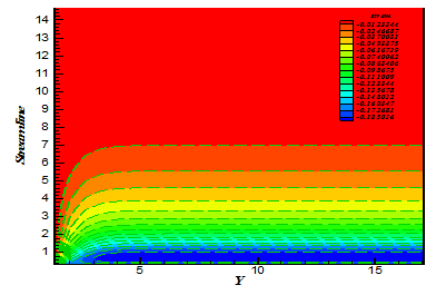
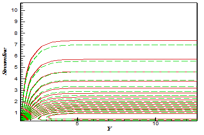
The non-dimensional equation after several transfigurations has been composed in the present numerical recitation. Therefore, for this contention, X and Y axis are dimensionless which announces the mesh extremity that has a great distance from the numerical calculation. In addition, with the stream and isotherms (line view) curves, the disparity of boundary layer for several parameters can be demarcated. The upliftment of streamlines and isotherms are submitted in Figure (23-24). It can be viewed that, thermal boundary layer and momentum boundary layer decreases due to the increase of radiation parameter, but the reverse trend is observed for the Chemical reaction parameter.
Table 1. Variation of parameters on skin friction coefficient, Nusselt number and Sherwood number
|
Kr |
Sc |
M |
Cf |
Nu |
Sh |
|
0.20 |
|
|
-3.73757 |
1.33590 |
4.30353 |
|
2.00 |
|
|
-3.74333 |
1.33231 |
4.44471 |
|
4.00 |
|
|
-3.74893 |
1.32883 |
4.58066 |
|
6.00 |
|
|
-3.75438 |
1.32547 |
4.71161 |
|
|
2.60 |
|
-3.73757 |
1.33590 |
4.30353 |
|
|
5.60 |
|
-3.78171 |
1.30935 |
5.23563 |
|
|
8.60 |
|
-3.79747 |
1.29918 |
5.59656 |
|
|
11.60 |
|
-3.80556 |
1.29383 |
5.78717 |
|
|
|
2.00 |
-3.73757 |
1.33590 |
4.30353 |
|
|
|
4.00 |
-3.83048 |
1.33590 |
4.30353 |
|
|
|
6.00 |
-3.92086 |
1.33590 |
4.30353 |
|
|
|
8.00 |
-4.00879 |
1.33590 |
4.30353 |
Table 2. Variation of diversified parameters (Du and So) on skin friction coefficient, Nusselt number and Sherwood number.
|
Du |
So |
Cf |
Nu |
Nt |
|
0.20 |
|
-3.75712 |
1.13380 |
4.78790 |
|
0.80 |
|
-3.77945 |
0.87497 |
5.38131 |
|
0.85 |
|
-3.87586 |
0.82512 |
5.49260 |
|
0.90 |
|
-3.87993 |
0.77309 |
5.60779 |
|
|
2.60 |
-3.73757 |
1.33590 |
4.30353 |
|
|
3.60 |
-3.67566 |
1.35809 |
3.55242 |
|
|
4.60 |
-3.61180 |
1.38169 |
2.75198 |
|
|
6.60 |
-3.47786 |
1.43350 |
0.98864 |
Table 3. Previous results by Venkateswarlu et al. (2017)
|
Increased parameter |
Velocity Profile |
Temperature profile |
Concentration Profile |
Skin friction |
Nussselt number |
Sherwood number |
|
M |
Dec |
|
|
|
|
|
|
Du |
|
|
|
Inc |
Inc |
Inc |
|
R |
Dec |
Inc |
Dec |
|
|
|
|
So |
Inc |
Dec |
Inc |
|
|
|
Table 4. Present results
|
Increased parameter |
Velocity Profile |
Temperature profile |
Concentration Profile |
Skin friction |
Nussselt number |
Sherwood number |
|
M |
Dec |
|
|
Dec |
|
|
|
So |
Inc |
|
Inc |
Inc |
|
Dec |
|
Nb |
|
Inc |
|
|
|
|
|
Pr |
|
Dec |
Inc |
|
|
Dec |
|
Kr |
Dec |
|
|
|
|
|
|
Le |
Dec |
|
Dec |
|
|
|
|
Q |
|
Inc |
|
|
Dec |
|
Figure 3. Velocity profile for different values of Gm
Figure 4. Velocity profile for different values of Gr
Figure 5. Velocity profile for different values of Kr
Figure 6. Concentration profile for different value of Kr
Figure 7. Velocity profile for different values of M
Figure 8. Temperature profile for different values of Nb
Figure 9. Concentration profile for different values of Nb
Figure 10. Concentration profile for different values of Nt
Figure 11. Temperature profile for different values of Pr
Figure 12. Concentration profile for different values of Pr
Figure 13. Velocity profile for different values of Q
Figure 14. Temperature profile for different values of Q
Figure 15. Concentration profile for different values of Q
Figure 16. Velocity profile for different values of R
Figure 17. Concentration profile for different values of Sc
Figure 18. Velocity profile for different values of So
Figure 19. Concentration profile for different values of So
Figure 20. Skin friction profile for different values of So
Figure 21. Sherwood number profile for different values of So
Figure 22. Nusselt number profile for different values of Q
Figure 23. Stream line profile (Flood view) for different values of R
Figure 24. Stream line profile (Line view) for different values of R
The results are presented graphically and we conclude the following findings
(1) An enhancement in the radiation parameter R and chemical reaction parameter Kr conduct to decrease the velocity and concentration ordination.
(2) By increasing the Soret number enhances the velocity and concentration profiles.
(3) The surface temperature and concentration of a sheet increase with increasing values of magnetic field parameter M, but the velocity decreases with an increase in magnetic field number M due to the magnetic fascination of the Lorentz force acting on the flow field.
(4) The effect of heat source and radiation parameter on velocity profile is equivalent.
(5) The effect of So on skin friction and Sherwood number is opposite. But for the growing value of Q decreases the Nusselt number.
[1] Sakiadis, B.C. (1961). Boundary-layer behavior on a continuous solid surface: II. The boundary layer on a continuous flat surface. American Institute of Chemical Engineering, 7(2): 221-225. https://doi.org/10.1002/aic.690070211
[2] Hayat, T., Abbas, Z., Ali, N. (2008). MHD flow and mass transfer of a upper-convected Maxwell fluid past a porous shrinking sheet with chemical reaction species. Physics Letters A, 372(26): 4698-4704. https://doi.org/10.1016/j.physleta.2008.05.006
[3] Mustafa, M., Hayat, T., Alsaedi, A. (2015). Simulations for maxwell fluid flow past a convectively heated exponentially stretching sheet with nanoparticles. American Institute of Physics Advances, 5: 037133. https://doi.org/10.1063/1.4916364
[4] Abel, M.S., Tawade, J.V., Nandeppanavar, M.M. (2012). MHD flow and heat transfer for the upper-convected Maxwell fluid over a stretching sheet. Meccanica, 47: 385-393. https://doi.org/10.1007/s11012-011-9448-7
[5] Kmaran, G., Sandeep, N. (2016). Computaional analysis of magnetohydrodynamics Casson and Maxwell flows over a stretching sheet with cross diffusion. Results in Physics, 7: 147-155. https://doi.org/10.1016/j.rinp.2016.12.011
[6] Abbas, Z., Javed, T., Ali, N., Sajid, M. (2014). Flow and Heat Transfer of Maxwell Fluid over an Exponentially Stretching Sheet. Heat Transfer, 43(3): 233-242. https://doi.org/10.1002/htj.21074
[7] Hayat, T., Fetecau, C., Sajid, M. (2008). On MHD flow of a Maxwell fluid in a porous medium and rotating frame. Physics Letters A, 372(10): 1639-1644. https://doi.org/10.1016/j.physleta.2007.10.036
[8] Aliakbar, V., Alizadeh, A., Sadeghy, K. (2009). The influence of thermal radiation on MHD flow of maxwellian fluids above stretching sheets. Communications in Nonlinear Science and Numerical Simulation, 14(3): 779-794. https://doi.org/10.1016/j.cnsns.2007.12.003
[9] Zargartalebi, H., Ghalambaz, M., Noghrehabadi, A., Chamkha, A. (2015). Stagnation-point heat transfer of nanofluids towards stretching sheets with variable thermo physical properties. Advanced Powder Technology, 26: 819-82. https://doi.org/10.1016/j.apt.2015.02.008
[10] Khan, M.S., Rahman, M.M., Arifuzzaman, S.M., Biswas, P., Karim, I. (2017). Williamson fluid flow behavior of MHD convective radiative Catteno-Chirstov heat flux type over a linearly stretched surface with heat generationand thermal diffusion. Frontris in Heat and Mass Transfer, 9: 1-11. https://doi.org/10.5098/hmt.9.15
[11] Satya Narayan, P.V., Venkateswarlu, B., Venkataramana, S. (2013). Effects of hall current and radiation absorption on MHD micropolar fluid in a rotating system. Ain Shams Engineering Journal, 4: 843-854. https://doi.org/10.1016/j.asej.2013.02.002
[12] Nadeem, S., Haq, R.U., Khan, Z.H. (2014). Numerical solution of non-Newtonian nanofluid over a stretching sheet, Appl Nanosci, 4: 625-631. https://doi.org/10.1007/s13204-013-0235-8
[13] Nandy, S.K. (2015). Unsteady flow of a Maxwell fluid in the presence of nanoparticles towards a permeable shrinking surface with Navier slip. Journal of the Taiwan Institute of Chemical Engineering, 52: 22-30. https://doi.org/10.1016/j.jtice.2015.01.025
[14] Biswas, R., Mondal, M., Islam, A. (2019). A steady MHD natural convection heat transfer fluid flow through a vertical surface in the existence of Hall current and radiation. Instrumentation, Mesure, Métrologie, 2: 331-356. https://doi.org/10.3166/i2m.17.331-356
[15] Biswas, R., Ahmmed, S.F. (2018). Effects of Hall current and chemical reaction on MHD unsteady heat and mass transfer of Casson nanofluid flow through a vertical plate. Journal of Heat Transfer, 140(9). https://doi.org/10.1115/1.4039909
[16] Biswas, R., Mondal, M., Sarkar, D.R., Ahmmed, S.F. (2017). Effects of radiation and chemical reaction on MHD unsteady heat and mass transfer of Casson fluid flow past a vertical plate. Journal of Advances in Mathematics and Computer Science, 23(2): 1-16. https://doi.org/10.9734/JAMCS/2017/34292
[17] Biswas, R., Hasan, M., Mondal, M., Kazi Shanchia, M., Bulbul, F., Ahmmed, S.F. (2019). A numerical superintendence with stability exploration of Casson nanofluid flow in the effects of variable thermal conductivity and radiation. Advanced Science, Engineering and Medicine, 11(8): 697-707. https://doi.org/info:doi/10.1166/asem.2019.2413
[18] Hayat, T., Abbas, Z., Sajid, M. (2009). MHD flow of an upper-convected Maxwell fluid near a stagnation-point over a stretching surface. Chaos Solitons & Fractals, 39(2): 840-848. https://doi.org/info:doi/10.1016/j.chaos.2007.01.067
[19] Mukhopadhyay, S., Bhattacharyya, K. (2012). Unsteady flow of a Maxwell fluid over a stretching surface in presence of chemical reaction. Journal of the Egyptian Mathematical Society, 20: 229-234. https://doi.org/info:doi/10.1016/j.joems.2012.08.019
[20] Satya Narayan, P.V., Venkateswarlu, B., Venkataramana, S. (2015). Thermal radiation and heat source effects on a MHD nanofluid past a vertical plate in a rotating system with porous medium. Heat Transfer Asian Research, 44(1): 1-19. https://doi.org/info:doi/10.1002/htj.21101
[21] Satya Narayan, P.V., Venkateswarlu, B. (2016). Heat and mass transfer on MHD nanofluid flow past a vertical porous plate in a rotating system. Frontiers in Heat and Mass Transfer, 7(1): 8. http://dx.doi.org/10.5098/hmt.7.8
[22] Noor, N.F.M. (2012). Analysis for MHD flow of a Maxwell fluid past a vertical stretching sheet in the presence of thermophoresis and chemical reaction. International Journal of Mathematical, Computational, Physical, Electrical and Computer Engineering, 64: 1019-1023.
[23] Bishnoi, J., Goyal, N. (2012). Soret-Dufour driven thermosolutal instability of Darccy Maxwell fluid. International Journal of Engineering, 25(4): 367-378.
[24] Biswas, R., Afikuzzaman, M., Mondal, M., Ahmmed, S.F. (2018). MHD free convection and heat transfer flow through a vertical porous plate in the presence of chemical reaction. Frontiers in Heat and Mass Transfer, 11: 13.
[25] Biswas, R., Mondal, M., Shanchia, K., Ahmed, R., Abdus Samad, S.K., Ahmmed, S.F. (2019). Explicit finite difference analysis of an unsteady magnetohydrodynamics heat and mass transfer micropolar fluid flow in the presence of radiation and chemical reaction through a vertical porous plate. Journal of nanofluids, 8(7): 1583-1591. https://doi.org/10.1166/jon.2019.1704
[26] Biswas, R., Mondal, M., Hossain, S., Urmi, K.F., Suma, U.K., Katun, M. (2019). A numerical investigation with hydromagnetic stability convergence analysis on unsteady heat and mass transfer fluid flow through a vertical porous plate. Advanced Science, Engineering and Medicine, 11(8): 687-696. https://doi.org/10.1166/asem.2019.2411
[27] Biswas, R., Mondal, M., Sarkar, D.R., Ahmmed, S.F. (2017). Effects of radiation and chemical reaction on MHD unsteady heat and mass transfer of Casson fluid flow past a vertical plate. Journal of Advances in Mathematics and Computer Science, 23(2): 1-16. https://doi.org/10.9734/JAMCS/2017/34292
[28] Ahmmed, S.F., Biswas, R., Afikuzzaman, M. (2018). Unsteady magnetohydrodynamic free convection flow of nanofluid through an exponentially accelerated inclined plate embedded in a porous medium with variable thermal conductivity in the presence of radiation. Journal of Nanofluids, 7(5): 891-901. https://doi.org/10.1166/jon.2018.1520
[29] Ahmmed, S.F., Biswas, R. (2019). Effects of radiation and chemical reaction on MHD unsteady heat and mass transfer of nanofluid flow through a vertical plate. Modelling Measurement and Control B, 87(4): 213-220.
[30] Mondal, M., Biswas, M., Hasan, M., Shanchia, K., Ahmmed, S.F. (2019). Numerical investigation with stability convergence analysis of chemically hydromagnetic Casson nanofluid flow in the effects of thermophoresis and Brownian motion. International journal of heat and technology, 37(1): 59-70. https://doi.org/10.18280/ijht.370107
[31] Bilal Ashraf, M., Hayat, T., Alhuthali, M.S. (2016). Three dimensional flow of Maxwell fluid with Soret and Dufour effects. Journal of Aerospace Engineering, 29(3): 04015065. https://doi.org/10.1061/(ASCE)AS.1943-5525.0000551
[32] Narayana, P. S., Venkateswarlu, B., Venkataramana, S. (2013). Effects of Hall current and radiation absorption on MHD micropolar fluid in a rotating system. Ain Shams Engineering Journal, 4(4): 843-854. https://doi.org/10.1016/j.asej.2013.02.002