Kaniz Fatima Lima | Mahmud Alam
OPEN ACCESS
Fluid flow through a straight pipe in a rotating system with magnetic field acting along center line having hall current is investigated numerically. A cylindrical co-ordinate system has been employed to derive the steady two dimensional momentum equations. By using usual transformation, the steady two dimensional coupled nonlinear partial momentum equations are transferred into non-dimensional coupled nonlinear partial momentum equations. To solve these equations, the Spectral Method has been used as a main tool and the Collocation Method, Chybyshev Polynomial and Newton-Raphson Method are also used as the secondary tools. Also, Arc length Method is used to compute the critical zone results. The influence of magnetic parameter, hall parameter, pressure gradient parameter and rotating parameter, the nature of the total flow (flux) and stream line flow is investigated with different aspect ratios. The numerical technique is applied to solve the governing equations with the help of computer programming language Compaq visual FORTRAN 6.6a and visualize the secondary and axial flow with the help of Tecplot 360 (2009) and Gost Script 8.11 as well as Gost View 4.7 software’s for simulation as well as plotting. Finally the axial flow and stream line flow have been shown in contour and stream line format.
pressure gradient parameter, magnetic parameter, rotating parameter and hall parameter
The study MHD Fluid flow through a rectangular straight duct to rotate at a constant angular velocity about an axis normal to a plane including the pipe is subjected to both coriolis and centrifugal force. The attention on this field is considered because of its practical importance in chemical and mechanical engineering. Such rotating passages are used in the cooling system for conductors of electric generators and generator motors for pumped –storage stations. Dean [1, 2] was the pioneer to develop a mathematical model for the flow through a curved pipe under the fully developed flow conditions and studied at first on the motion of fluid in a curved pipe. The work on the flow in rotating straight pipe was carried out for the asymptotic limits of weak and strong rotations by Barua [3, 4]. Flow in rotating straight pipes of circular cross section studied by Ito and Nanbu [5] and Yamamoto et al. [6] with square cross section. Alam et al. [7] studied the effects of torsion, aspect ratio and curvature on the helical pipe with 0≤δ≤0.02. A stability analysis shows that all multiple solutions except the two-cell type are unstable which has been investigated by Winters [8]. Hall Effect is the production of a voltage difference across an electrical conductor, transverse to an electric current and a magnetic field perpendicular to the current. It is well known that the effect of Hall Current becomes significant at low density of an ionized fluid as stated by Cowling [9]. Hall currents effects are likely to be important in many astrophysical and geophysical simulations as well as in engineering problems such as Hall accelerators constructions of turbines and centrifugal machines. The Hall Effect on magnet was discovered by Edwin Herbert Hall [10] on a new action of the magnet on electric currents in his first work of doctoral degree at Johns Hopkins University in Baltimore, Maryland. Using finite difference method, the combined effect of Magnetic field and hall current have been studied with volumetric flow rate on the flow of a dusty Bingham fluid in a circular pipe by Hazem [11] and Afroja et al. (2015) worked on unsteady MHD viscous incompressible Bingham fluid flow. Using Spectral Methods [12] high torsion as well as rotation effect on fluid flow in a helical pipe with circular cross-section has been investigated by Masud and Alam [13] and the spiraling flow within a curved tube of rectangular cross-section normally formed two distinct cells in the plane of the cross-section and the bifurcation set and had a complex structure, with a number of higher-order singularities; the path of limit points have been found to cross in the manner of an unfolded swallowtail catastrophe. Wahiduzzaman et al. [14] worked on non-isothermal flow through a rotating straight duct with wide range of rotational and pressure driven parameters using spectral method. This investigation gradually studied by Hoque et al. [15] on fully developed flow and found the nature of the magnetohydrodynamics laminar flow in a rotating curved pipe with circular cross section. The effect of magnetic field on the fluid flow through a rotating straight duct with large aspect ratio has been studied by Kamruzzaman et al. [16]. The results for fully developed flow have been obtained by using Spectral method. The Arc length method has been used to obtain the critical zone results. Fluid flow has been investigated by Rina and Alam (2015) as well as Kadir and Alam [17] using the concept of hall current with magnetic field in a rotating parallel plate.
Hence our aim is to study on fluid flow through a straight pipe in a rotating system with magnetic field acting along the center line having hall current. Spectral Method is used as the main tool where Chebyshev polynomials, Collocation Methods and Newton Raphson method are used as secondary tools. Arc length method is used to calculate the results of critical solution zone. The results have been simulated for large aspect ratio and the results of axial velocity have been shown in the form of contour plots. Also the secondary velocity has been shown in the form of streamlines [18-21].
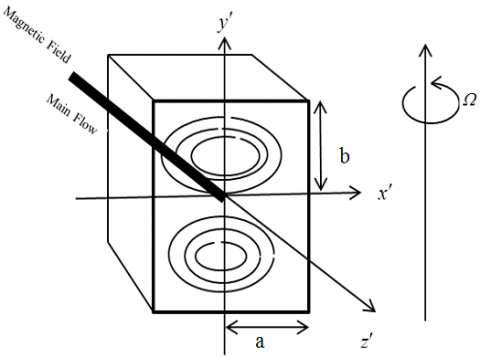
The fully developed laminar flow of an incompressible fluid in a straight pipe with rectangular cross-section in the presence of magnetic field including hall current is considered where $\Omega $ is the angular velocity for steady rotating system and $\mathbf{q}\left( u,v,w \right)$ is the fluid velocity vector in free dimensionless Cartesian co-ordinate system. Consider $2a$ is the cross-sectional width of the pipe and $2b$ is considered its height.
Equation yields in vector form as follows:
$\nabla .\mathbf{q}=0$ (1)
$\frac{d \boldsymbol{q}}{d t}=\boldsymbol{F}-\frac{1}{\rho} \nabla p+v \nabla^{2} q$ (2)
Figure 1. Co-ordinate system of a rotating straight pipe
Cartesian co-ordinate system $\left( {x}',{y}',{z}' \right)$ has been considered to describe the motion of the fluid particles in the pipe which is described in Figure 1. The system rotates with angular velocity $\mathbf{\Omega }=\left( 0,-\Omega ,0 \right)$ around the y-axis. The flow is driven by pressure gradient $-\frac{\partial {p}'}{\partial {z}'}=G$ along the centerline of the pipe in the presence of magnetic field and hall current. When fluid moves along the electric and magnetic field as well as a uniform magnetic field $\mathbf{B}$ is applied in a rotating straight pipe with rectangular cross-section along the center line, it becomes as follows
$\frac{\partial \bar{q}}{\partial t}+\bar{q}\left( \bar{q}.\bar{\nabla } \right)=\mathbf{F}-\frac{1}{\rho }\nabla p+\upsilon {{\nabla }^{2}}q+2\left( \mathbf{\Omega }\,\wedge \,\,\mathbf{q} \right)+\frac{1}{\rho }\left( \mathbf{J}\wedge \mathbf{B} \right)$ (3)
$J\wedge B$ is the force on the fluid per unit volume produced by interaction of the electric and magnetic field(called Lorentz Force). $\upsilon $ is the kinematic viscosity and $\mathbf{q}$ is the fluid velocity in the pipe.
The generalized Ohm’s Law in the absence of electric field is of the form
$\boldsymbol{J}+\frac{\omega_{e} \tau_{e}}{B_{0}} \boldsymbol{J} \wedge \boldsymbol{B}=\sigma^{\prime}\left(\mu_{e} \boldsymbol{q}^{\prime} \wedge \boldsymbol{B}+\frac{1}{e n_{e}} \nabla p_{e}\right)$ (4)
where ${{\omega }_{e}}$ is the cyclotron frequency, ${{\tau }_{e}}$ is the electron collision, $e$ is the electric charge, $n$ is the number density electron. Here ${{\omega }_{e}}{{\tau }_{e}}=m$ is the hall parameter and ${{p}_{e}}=0.$
$\frac{\partial u^{\prime}}{\partial x^{\prime}}+\frac{\partial v^{\prime}}{\partial y^{\prime}}+\frac{\partial w^{\prime}}{\partial z^{\prime}}=0$ (5)
The Radial Momentum equation
$u^{\prime} \frac{\partial u^{\prime}}{\partial x^{\prime}}+v^{\prime} \frac{\partial u^{\prime}}{\partial y^{\prime}}+w^{\prime} \frac{\partial u^{\prime}}{\partial z^{\prime}}=-\frac{1}{\rho} \frac{\partial p^{\prime}}{\partial x^{\prime}}+v\left(\frac{\partial^{2} u^{\prime}}{\partial x^{\prime 2}}+\frac{\partial^{2} u^{\prime}}{\partial y^{\prime 2}}+\frac{\partial^{2} u^{\prime}}{\partial z^{\prime 2}}\right)-2 \Omega v^{\prime}-\frac{\sigma B_{0}^{2}}{\rho}\left(\frac{u^{\prime}+m v^{\prime}}{1+m^{2}}\right)$ (6)
The Vertical Momentum equation
$u^{\prime} \frac{\partial v^{\prime}}{\partial x^{\prime}}+v^{\prime} \frac{\partial v^{\prime}}{\partial y^{\prime}}+w^{\prime} \frac{\partial v^{\prime}}{\partial z^{\prime}}=-\frac{1}{\rho} \frac{\partial p^{\prime}}{\partial y^{\prime}}+v\left(\frac{\partial^{2} v^{\prime}}{\partial x^{\prime 2}}+\frac{\partial^{2} v^{\prime}}{\partial y^{\prime 2}}+\frac{\partial^{2} v^{\prime}}{\partial z^{\prime 2}}\right)+\frac{\sigma B_{0}^{2}}{\rho}\left(\frac{m u^{\prime}-v^{\prime}}{1+m^{2}}\right)$ (7)
The Axial momentum equation is
$u^{\prime} \frac{\partial v^{\prime}}{\partial x^{\prime}}+v^{\prime} \frac{\partial w^{\prime}}{\partial y^{\prime}}+w^{\prime} \frac{\partial v^{\prime}}{\partial z^{\prime}}=-\frac{1}{\rho} \frac{\partial p^{\prime}}{\partial z^{\prime}}+v\left(\frac{\partial^{2} w^{\prime}}{\partial x^{\prime 2}}+\frac{\partial^{2} w^{\prime}}{\partial y^{\prime 2}}+\frac{\partial^{2} w^{\prime}}{\partial z^{\prime 2}}\right)+2 \Omega u^{\prime}$ (8)
Here the axis of rotation is perpendicular to the span of the pipe and the axial pressure gradient $-\frac{\partial {p}'}{\partial {z}'}=G$ is constant and is maintained by external means i.e ${p}'$ is the modified pressure, which includes the gravitational and centrifugal force potentials. The axial pressure gradient $G=\frac{\partial {p}'}{\partial {z}'}$ is substituted in (8), the equation becomes
$\frac{\partial {w}'}{\partial t}+{u}'\frac{\partial {w}'}{\partial {x}'}+{v}'\frac{\partial {w}'}{\partial {y}'}+{w}'\frac{\partial {w}'}{\partial {z}'}=\frac{G}{\rho }+\upsilon \left( \frac{{{\partial }^{2}}{w}'}{\partial {{{{x}'}}^{2}}}+\frac{{{\partial }^{2}}{w}'}{\partial {{{{y}'}}^{2}}}+\frac{{{\partial }^{2}}{w}'}{\partial {{{{z}'}}^{2}}} \right)+2\Omega {u}'\,$
The boundary conditions are that ${u}'={v}'={w}'=0$ on the wall of the straight duct. The assumption of fully developed flow means that except for the pressure derivative all ${z}'$ derivatives are set to zero. The following dimensionless variables have been used to obtain the dimensionless equation and the above equations becomes
${u}'=\frac{\upsilon }{a}u\,;\,\,\,{x}'=xa\,;\,\,\,{p}'=\frac{{{\upsilon }^{2}}}{{{a}^{2}}}\rho p\,\,;\,\,\,\,{v}'=\frac{\upsilon }{a}v\,\,;\,\,\,{y}'=ya\,\,;\,\,\,{w}'=\frac{\upsilon }{a}w\,\,;\,\,\,{z}'=0$
The boundary condition is that the velocities are zero at $x=\pm 1$ and $y=\pm \frac{b}{a}=\gamma $(aspect ratio).It is introduced the new variable $\bar{y}=\left( \frac{y}{\gamma } \right),$ where $\gamma $ is the aspect ratio i.e $\gamma =\left( \frac{b}{a} \right),$ where $b$ be the half height of the cross section and $u=-\left( \frac{\partial \psi }{\partial y} \right)$ and $v=-\left( \frac{\partial \psi }{\partial x} \right)$ which satisfies the continuity equation.
Rotating parameter ${{T}_{r}}=2\left( \frac{{{a}^{2}}\Omega }{\upsilon } \right),$ Magnetic Parameter ${{M}_{g}}=\frac{{{\sigma }'}}{{{\mu }_{e}}}{{a}^{2}}{{B}_{0}}^{2}={\sigma }'{{\mu }_{e}}{{a}^{2}}{{H}_{0}}^{2},$ Pressure driven parameter ${{D}_{n}}=\frac{G{{a}^{3}}}{\rho {{\upsilon }^{2}}}$ The dimensionless governing equations for $\psi $ and $w$ are as follows:
$\frac{{{\partial }^{4}}\psi }{\partial {{x}^{4}}}+\frac{2}{{{\gamma }^{2}}}\frac{{{\partial }^{4}}\psi }{\partial {{{\bar{y}}}^{2}}\partial {{x}^{2}}}+\frac{1}{{{\gamma }^{4}}}\frac{{{\partial }^{4}}\psi }{\partial {{{\bar{y}}}^{4}}}=-\frac{1}{{{\gamma }^{3}}}\frac{\partial \psi }{\partial \bar{y}}\frac{{{\partial }^{3}}\psi }{\partial x\partial {{{\bar{y}}}^{2}}}-\frac{1}{\gamma }\frac{\partial \psi }{\partial \bar{y}}\frac{{{\partial }^{3}}\psi }{\partial {{x}^{3}}}+\frac{1}{{{\gamma }^{3}}}\frac{\partial \psi }{\partial x}\frac{{{\partial }^{3}}\psi }{\partial {{{\bar{y}}}^{3}}}+\frac{1}{\gamma }\frac{\partial \psi }{\partial x}\frac{{{\partial }^{3}}\psi }{\partial {{x}^{2}}\partial \bar{y}}-\frac{1}{\gamma }\frac{\partial w}{\partial \bar{y}}{{T}_{r}}+\frac{{{M}_{g}}}{1+{{m}^{2}}}\left( \frac{1}{{{\gamma }^{2}}}\frac{{{\partial }^{2}}\psi }{\partial {{{\bar{y}}}^{2}}}+\frac{{{\partial }^{2}}\psi }{\partial {{x}^{2}}} \right)\,$ (9)
$\frac{{{\partial }^{2}}w}{\partial {{x}^{2}}}+\frac{1}{{{\gamma }^{2}}}\frac{{{\partial }^{2}}w}{\partial {{{\bar{y}}}^{2}}}=-\frac{1}{\gamma }\frac{\partial \psi }{\partial \bar{y}}\frac{\partial w}{\partial x}+\frac{1}{\gamma }\frac{\partial \psi }{\partial x}\frac{\partial w}{\partial \bar{y}}-{{D}_{n}}+\frac{1}{\gamma }\frac{\partial \psi }{\partial \bar{y}}{{T}_{r}}$ (10)
The boundary conditions are as follows:
$w\left( \pm 1,\bar{y} \right)=w(x,\pm 1)=\psi \left( \pm 1,\bar{y} \right)=0$
$\left( \frac{\partial \psi }{\partial x} \right)\left( \pm 1,\bar{y} \right)=\psi \left( x,\pm 1 \right)=\left( \frac{\partial \psi }{\partial \bar{y}} \right)\left( x,\pm 1 \right)=0$
Spectral methods have proven a powerful tool in simulation of incompressible steady flow. This work is based on Spectral methods and Collocation methods. The Collocation method has been used to discretize the cross section of the pipe and used in vertical and radial directions. The series of Chebyshev polynomials and Newton Raphson method are used to solve the non-linear differential equations in $\bar{x}$ and $\bar{y}$ directions. Actually the expansion by polynomial function is utilized to obtain steady or unsteady solution. The symmetric solution of the rotating pipe is expressed as secondary flow and contour plots of axial flow which are expended as:
${{\varphi }_{n}}(x)=\left( 1-{{x}^{2}} \right){{T}_{n}}(x),{{\psi }_{n}}(x)={{\left( 1-{{x}^{2}} \right)}^{2}}{{T}_{n}}(x)$
where ${{\varphi }_{n}}(x)$ and ${{\psi }_{n}}(x)$ are expansion function. ${{T}_{n}}(x)=\cos \left( n{{\cos }^{-1}}(x) \right)$ is ${{n}^{th}}$ order first kind Chebyshev Polynomial. $w(x,\bar{y})$ and $\psi (x,\bar{y})$ are expressed in terms of ${{\varphi }_{n}}\left( x \right)$ and ${{\psi }_{n}}\left( x \right)$.
$w(x,\bar{y})=\sum\limits_{m=0}^{M}{\sum\limits_{n=0}^{N}{{{w}_{mn}}{{\varphi }_{m}}(x){{\varphi }_{n}}}}(\bar{y})$
$\psi (x,\bar{y})=\sum\limits_{m=0}^{M}{\sum\limits_{n=0}^{N}{{{\psi }_{mn}}{{\psi }_{m}}(x){{\psi }_{n}}}}(\bar{y})$
where $M$ and $N$ are truncation number in the $x$ and $\bar{y}$ directions respectively. The collocation points are taken as $({{x}_{i}},{{\bar{y}}_{j}})$
${{x}_{i}}=\cos \left[ \pi \left( 1-\frac{i}{M+2} \right) \right],{{y}_{j}}=\cos \left[ \pi \left( 1-\frac{j}{M+2} \right) \right]$
where $i=1,2,3,4,...,M+1$ and $j=1,2,3,4,...,N+1$. The obtained non-linear algebraic equations are solved by the Newton-Raphson iteration method as follows:
${{w}^{\left( p+1 \right)}}={{C}_{1}}^{-1}{{N}_{1}}\left( {{w}_{mn}}^{\left( p \right)},\,{{\psi }_{mn}}^{\left( p \right)} \right),\,\,{{\psi }^{\left( p+1 \right)}}={{C}_{2}}^{-1}{{N}_{2}}\left( {{w}_{mn}}^{\left( p \right)},\,{{\psi }_{mn}}^{\left( p \right)} \right)$
where $p$ denotes the iteration number. The arc-length equation is
$\sum\limits_{m=0}^{M}{\sum\limits_{n=0}^{N}{\left[ {{\left( \frac{d{{w}_{mn}}}{ds} \right)}^{2}}+{{\left( \frac{d{{\psi }_{mn}}}{ds} \right)}^{2}} \right]}}=1$
which is solved by using the Newton-Raphson iteration method. An initial guess at a point $s+\Delta s$ is considered as:
${{w}_{mn}}(s+\Delta s)={{w}_{mn}}(s)+\frac{d{{w}_{mn}}(s)}{ds}\Delta s,\,\,{{\psi }_{mn}}(s+\Delta s)={{w}_{mn}}(s)+\frac{d{{\psi }_{mn}}(s)}{ds}\Delta s$
To obtain a correct solution at $s+\Delta s$ the convergence is taken ${{\varepsilon }_{p}}<{{10}^{-8}}$ which is defined as:
${{\varepsilon }_{p}}={{C}_{1}}^{-1}{{N}_{1}}{{\left( {{w}_{mn}}^{\left( p+1 \right)}-{{w}_{mn}}^{\left( p \right)} \right)}^{2}}+{{\left( {{\psi }_{mn}}^{\left( p+1 \right)}-{{\psi }_{mn}}^{\left( p \right)} \right)}^{2}}$
Fully developed flow implies that the velocity distribution does not change in the direction of fluid when the velocity of the fluid for a fully developed flow is fastest at the center line of the pipe and the velocity at the walls of the pipe is slowest. In such a case, the pressure in the flow direction balance the shear stress near the wall but momentum changes only in the radial direction. The main flow is imposed by the Hall Current in the presence of magnetic field (Figure 1) along the center line of the rotating straight pipe. Co-rotation and counter clockwise rotation are considered. The flow characteristics are investigated by using different Pressure gradient parameters $\left( {{D}_{n}} \right),$ and Hall parameters $\left( m \right)$ at different aspect ratios in the presence of rotating parameter and magnetic parameter. The truncation number $M$and $N$with aspect ratios are changed for numerical calculation to make different cross-section of the pipe. For a good accuracy of the solutions, $N$ is chosen equal to $\gamma M.$ The physical problem has been solved by using Spectral Method as main tool and Newton Raphson Iteration Method, Chebyshev Polynomial and Collocation Method are used as secondary tools. Critical solution zone of the solution curve is obtained by Arc-length method where the solutions are not converged as usual. Arc-length method has been extrapolated the singular points like bifurcation points. To obtain the appropriate result Mesh sensitivity test, Convergence test and validation test are required to know the validity and comparision of the present work. The Present study has aimed to reveal the nature of flux and emphasized on the effects of Pressure Gradient pressure in the presence of Hall Current.
4.1 Mesh Sensitvity Test
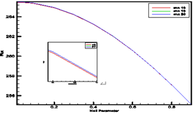
To obtain an appropriate and better result mesh spaces are taken $m=10,n=10$ and $m=16,n=16$ as well as $m=20,n=20,$ the computations have been carried out for three different mesh sizes which is shown in Figure 2. The mesh results are quietly same with the mesh sizes. The curves are smooth for all mesh spaces and show a negligible changes among the curves. space.This test is called Mesh sensitivity test.
4.2 Convergence Test
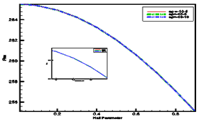
To obtain the above mentioned steady-state solution of the developed mathematical model, the computations are observed that the result of computations for differentconvergence parameters ${{10}^{-5}},\,{{10}^{-8}},{{10}^{-10}}$ are examined to test the convergence by using the techniq and defined as Convergence Parameter $ep.$ However, this computation shows almost same result and convergesto the point. It is observed that the result of computationsfor different parameters shows little changes after ${{10}^{-5}}$ and shows negligible changes after ${{10}^{-8}}$ and ${{10}^{-10}}$.
Figure 2. Mesh sensitivity test
Figure 3. Convergence test
4.3 Validation Sensitivity Test(Comparison)
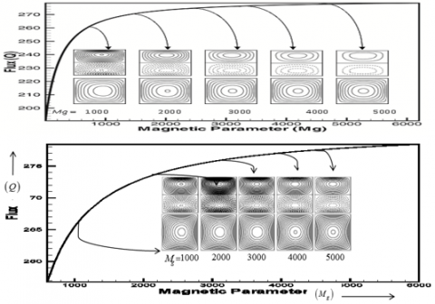
A validation test of the present study with magnetic parameters and the results of Kamruzzaman et al. [146] are shown in Figure 4. These results are qualitatively same but not quantitavely. Contour lines and streamlines plot have been obtained different for the effect of Hall Parameters in the present study. The computational results of Visual Studio Developer FORTRAN 6.6a and Gost Scripts 8.11 and Gost View 4.7 are almost same.
Figure 4. Validation Test of Previous work with Present work
These tests have been assured to investigate the present work where Hall current has been applied. Two cases are considered as:
Case-I
Case-II
Case I: Variation of Pressure Gradient Parameter at aspect ratio $\gamma =1.0$
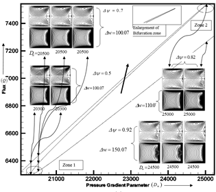
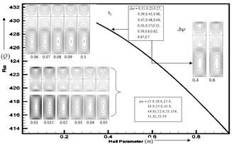
This comprehensive estimation obtains a steady solution curves along the center line for total flow $\left( Q \right)$ versus Pressure Gradient Parameter $\left( {{D}_{n}} \right)$ when Hall Parameter $\left( m \right)=0.5,$ Magnetic Parameter $\left( {{M}_{g}} \right)=1000$ and Rotating Parameter $\left( {{T}_{r}} \right)=1000$. Pressure Gradient Parameter $\left( {{D}_{n}} \right)$ is reached up to the range $50\le {{D}_{n}}\le 23500,\,\,50\le {{D}_{n}}\le 3500,\,\,50\le {{D}_{n}}\le 2500$ with regard to aspect ratios $\gamma =1.0,\,2.0,\,3.0$ respectively where steady solutions are found by applying Spectral Method, Collocation Method and Chebyshev as well as critical solution zones are found by Arc-length Method in the range $23500\le {{D}_{n}}<25500,\,\,3500\le {{D}_{n}}\le 11473,\,2500\le {{D}_{n}}\le 7800$ respectively for $\gamma =1.0,\,2.0,\,3.0$ which have been described in Figures 5-7. The main flow is forced by the magnetic field along the center line and Hall Current and Pressure Gradient are produced from here. An assessment on the fluid flow through a straight pipe is completed over the parametric space. The variation of the secondary flow and the axial flow at the several Pressure Gradient Parameters $\left( {{D}_{n}} \right)$on the solution curves are drawn for constants $\psi $ and $w$ in a cross-section of the pipe; looked the figures from the upstream. The right hand side of each pipe box is in the outside direction of the pipe from the center line. In the figures of secondary flow, solid lines $\left( \psi >1 \right)$ show that the secondary flow is in the counter clockwise direction while the dotted ones $\left( \psi <1 \right)$ show that the flow is in the clockwise direction. The streamlines and contour lines of Pressure Gradient Parameters $\left( {{D}_{n}} \right)$ are detected by arrow sign on the steady solution curve. Flux increases with the increase of Pressure Gradient Parameter $\left( {{D}_{n}} \right).$ Specially Two Bifurcation zones are found in aspect ratio $\gamma =1.0$ in Figure 5.
The two Bifurcation zones are obtained where zone 2 has enlarged in Figure 5. Three flux points on the curve are delineated on Bifurcation zone 2 (critical solution zone) to perceive of the identical Pressure Gradient Parameter ${{D}_{n}}=24500$ respectively where the distance between contour lines and streamlines plot are obtained $150.07$ and $0.92$. Four vortex solutions are acquired. Meanwhile two flux points on the curve are taken for same Pressure Gradient Parameter ${{D}_{n}}=25000$ on the Bifurcation zone 2 where distance between contour lines and streamlines plot are $110.07$ and $0.82$ and four vortex solutions have been found at each flux point. In bifurcation zone 1, distance between contour lines and streamlines plot are considered $\Delta w=100.07 $ and $\Delta \psi =0.7$ to find out vortex solution on the flux point for Pressure Gradient Parameter $\left( {{D}_{n}} \right)=20500.$ Arrow sign is used to detect the point on the bifurcation zone 1 of the curve and four vortex solutions have been found at each streamline plot. The contour lines are shifted to the outer wall. There are examined the nature of contour lines and streamlines plot to achieve different flux points on the curve with respect to the indistinguishable point of Pressure Gradient Parameter $\left( {{D}_{n}} \right)=20300$. The distance between contour lines and streamlines plot are considered $\Delta w=100.07$ and $\Delta \psi =0.7.$ respectively.
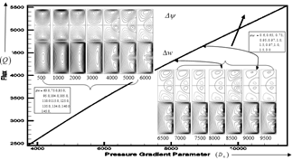
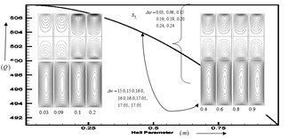
Solutions curve of Pressure Gradient Parameter $\left( {{D}_{n}} \right)$ have been delineated in the Figure 6 with respect to total flow $\left( Q \right)$ by imposing Arc-length Method. Stream lines of the secondary flow and contour plot of axial flow have been drawn in Figure 6 where distance between contour lines and streamlines plot are considered $\Delta w=63.0,\,\,75.0,\,\,85.0,\,\,95.0,104.0,\,105.0,\,110.0$ and $\Delta \psi =0.6,\,\,0.65,\,\,0.75,\,\,0.95,\,0.97,\,1.0,\,1.5$ respectively with respect to the Pressure Gradient Parameters $\left( {{D}_{n}} \right)=500,1000,2000,3000,$ 3500, 4000, and 5000 at aspect ratio $\gamma =2.0.$Again other Pressure Gradient Parameters $\,6000,\,6500,\,7000,\,8000,\,9000,\,\,9500$ are considered when distance between contour lines and streamlines plot are taken $\Delta w=115.0,\,\,125.0,\,\,135.0,134.0,\,\,140.0,\,$ $145.0,\Delta \psi =0.97,\,1.0,\,$ $1.5,\,2.0,\,\,2.5,\,\,\,3.0$ respectively. Instead of a large difference in the streamlines plot solid lines are found and two and four vortex solutions have been obtained with the change of Pressure Gradient Parameters on the solution curve of flux.
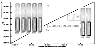
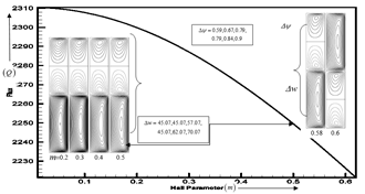
Steady solution curve has been obtained in the numerical scale $50\le {{D}_{n}}\le 7800$ at aspect ratio $\gamma =3.0.$ The streamlines plots $\psi $ and the contour lines $w$have been drawn in Figure 7 with increment of Pressure Gradient Parameters ${{D}_{n}}=1000,\,\,2000,\,\,3000,\,\,4000,\,\,5000,\,\,6000,\,\,7000$ $\Delta \psi =0.3,\,\,\,0.4,\,\,0.45,\,\,0.5,\,\,0.6,\,\,0.7,\,0.79$ and $\Delta w=19.0,\,\,\,37.0,\,\,50.0,\,\,70.0,\,\,85.0,\,\,95.0,\,\,109.0$ respectively Two vortex solutions have been obtained in this case. The maximum axial flow is shifted to the outer wall from center of the pipe cross-section. The solid lines and dashed lines of the streamlines plot are much thicker with the increase of Pressure Gradient Parameters than the previous streamlines plot of aspect ratios $\gamma =1.0,\,2.0.$
Figure 5. Solution curve for flux (Q) versus Pressure Gradient Parameters Dn=20300,20500, 24500,25000 at m=0.5, Mg=1000 and Tr=50.79;
Figure 6. Solution curve for total flow (Q) versus Pressure Gradient Parameters Dn=500,1000,2000, 3000,4000,5000,6000,6500,7000,7500,8000,8500,9000,9500 at m=0.5,Mg=1000,Tr=50.79,γ=2.0;
Figure 7. Solution curve for total flow (Q) versus Pressure Gradient Parameters Dn=1000,2000, 3000,3500,4000,5000,6000 at m=0.5, Mg=1000, Tr=50.79,γ=3.0
Case II: Variation of Hall Parameter m at aspect ratio γ=1.0 and Mg=1000
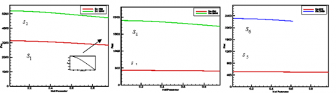
Figure 8 illustrates the steady solution curves s1,s2,s3,s4,s5.s6 for flux (total flow) (Q) versus Hall Parameter (m) where flux decreases with the increase of Hall Parameter (m).The secondary flow and axial flow at several values of m are reached up to 0.01≤m<1.0 by their restriction.
Figure 8. Steady solution curves for total flow (Q) versus Hall Parameter (m) at Aspect Ratios γ=1.0,2.0,3.0 and Tr=50.79, Dn=6000,15000,500,2500,500,2500
Figure 9. Solution curve for flux (Q) (total flow) versus Hall Parameter (m) at Dn=15000, Mg=1000,Tr=50.79 where Hall Parameters (m) are 0.02,0.05,0.06,0.08,0.1,0.2,0.3,0.5,0.6, 0.7,0.8,0.9
Steady solution curves s1 have been demonstrated and enlarged in Figure 8 to show the same nature of flux for other solutions curve. The other steady solution curve has been illustrated in Figure 9 and describe the nature of flux which decreases with the raise of Hall Parameter up to its range (m<1.0.). Secondary flow and axial flow on the curve have been obtained where distance between contour lines and stream lines plot are taken 56.07 (bottom) in the axial flow and 0.457 (top) in the secondary flow respectively. In this case Hall Parameters are considered m=0.02,0.05,0.06, 0.08,0.1, 0.2,0.3,0.5,0.6,0.7,0.8,0.9 at Pressure Gradient Parameter Dn=15000 respectively. The contour lines are shifted to the outer wall. Arrow sign has been used to detect the point of Hall Parameters on the solution curve.
iii. Aspect Ratio γ=2.0
The steady solution is found on the solution curves s3, s4 for Pressure Gradient Parameters Dn=500,2500 in the range of Hall Parameters 0.01≤m<1.0 when other parameters Mg=1000, Tr=50.79 remain constant.
In Figures (10-11), the total flow (Q) decreases with the increase of Hall Parameter (m) which is the new findings from the previous work. On the steady solution curve s3 Hall parameters are considered m=0.01, 0.015,0.02,0.03,0.04,0.05,0.06,0.07,0.08,0.09,0.1, 0.3,0.4, 0.5, 0.6,0.8,0.9 at Pressure Gradient Parameter Dn=500 in Figure 10. The contour lines and streamlines plot are drawn on the curve where distance between streamlines ψ and contour lines w have been taken with increment=0.15,0.23,0.27,0.39,0.45,0.46,0.47,0.48,0.49,0.50,0.57,0.55,0.59,0.6,0.62,0.67,0.7, Δw=15.0,15.0,15.0,20.0,25.0,30.0,35.0,43.0,49.0,49.03,52.0,52. 01,53.359,53.39,53.42,53.50. Arrow sign has been used to detect the point of Hall Parameters m=0.4,0.5,0.8.
On the solution curve s4 distance between contour lines and streamlines plot are 49.03, 49.05, 49.03, 52.0, 53.05, 53.05, 53.359, 53.39, 53.42, 53.42, 53.50 and 0.39, 0.45, 0.46, 0.47, 0.48, 0.49, 0.5, 0.59, 0.6, 0.62, 0.67 where Hall parameters are considered 0.02,0.05,0.09,0.1,0.2, 0.3,0.4,0.5, 0.6,0.8,0.9. at Pressure Gradient Parameter Dn=2500 in Figure 11.
Figure 10. Solution curve for flux Q (total flow) versus Hall parameter (m) at Pressure Gradient Parameter Dn=500, Magnetic Parameter Mg=1000, Rotating Parameter Tr=50.79 where Hall Parameters are m=0.01, 0.015,0.02,0.03,0.04,0.05, 0.06,0.07,0.08,0.09,0.1,0.2,0.3,0.4.0.6
Figure 11. Solution curve for flux Q (total flow) versus Hall parameter (m) at Pressure gradient parameter Dn=2500, Magnetic Parameter Mg=1000, Rotating parameter Tr=50.79 where Hall parameters are considered m=0.02,0.05,0.09, 0.1,0.2.0.3,0.4,0.5, 0.6,0.8,0.9
iii. Aspect Ratio γ=3.0
The steady solution curves s5, s6 are obtained for Pressure Gradient Parameters Dn=500, 2500 in the range of Hall Parameters 0.01≤m<1.0 when other Parameters Mg=1000, Tr=50.79 remain constant. One steady solution curve is enlarged at Dn=500 to show the nature of all steady curves in Figure12 and denoted by arrow sign. In Figures. (12-13) the total flux (Q) decreases with the increase of Hall Parameter (m).
Dn=500,2500
On the solution curve s5 Hall parameters are considered m=0.03,0.09,0.1,0.2,0.4,0.6,0.8,0.9 at Pressure Gradient Parameter Dn=500n showing in Figure 13. Arrow sign have been used to detect the point of Hall Parameters m=0.4. Two vortex solutions have been found in each case. Distance between contour lines and streamlines plots are Δw=15.0, 15.0, 16.0, 16.0, 16.0, 17.05, 17.05, 17.05 and Δψ=0.03, 0.09, 0.15, 0.19, 0.19, 0.20, 0.24, 0.24 respectively.
Figure 12. Solution curve for flux Q (total flow) versus Hall parameter (m) at Pressure gradient parameter
Magnetic Parameter Mg=1000, Rotating parameter Tr=50.79 where Hall parameter m=0.03,0.09,0.1, 0.2,0.4,0.6,0.8,0.9On the solution curve s6 Hall parameters are considered m=0.2,0.3, 0.4,0.5,0.58,0.6 at Pressure Gradient Parameter Dn=2500 showing in Figure 13. Distance between streamlines ψ and contour lines
have been taken with increment Δψ=0.59,0.67,0.79,0.79,0.84,0.9, Δw=45.07, 45.07,57.07,45.07,62.07,70.07. Arrow sign have been used to detect the point of Hall Parameters m=0.4. Two vortex solutions have been found in each case.Figure 13. Solution curve for flux Q (total flow) versus Hall parameter (m) at Pressure gradient parameter Dn=2500, Magnetic Parameter Mg=1000, Rotating parameter Tr=50.79 where Hall parameters m=0.2,0.3,0.4,0.5, 0.58,0.6
From the numerical investigation, the following inferences can be drawn:
The steady solutions have been obtained in different values of Pressure Gradient Parameter (Dn), Magnetic Parameter (Mg) and Hall Parameter (m), Flux (Q) increases with the increase of Pressure Gradient Parameter (Dn). Two vortex and four vortex solutions have been obtained. The strength of the secondary flow pattern especially Bifurcation zone is obtained for aspect ratio γ=1.0 and four vortex solutions are found.
Flux (Q) decreases with the increase of Hall Parameter (m) and two vortex solutions have been obtained of all the secondary flow. The fluid particles motion strength is weak in the flow patterns of the secondary flow. The middle of the secondary flow is vacuum with the increase of aspect ratios.
The present study has aimed to reveal the nature of flux and emphasized on the effects of Pressure Gradient Parameter and Magnetic Parameter in the presence of Hall Current.
|
$F$ |
Body force |
|
$G$ |
Non-dimensional pressure driven parameter |
|
$R$ |
Non-dimensional rotation parameter |
|
$q$ |
Fluid velocity |
|
$p$ |
Fluid pressure |
|
$p'$ |
Modified fluid pressure |
|
$a$ |
Half width of the duct cross-section |
|
$b$ |
Half-height of the duct cross-section |
|
$M_{g}$ |
Magnetic parameter |
|
$m$ |
Hall parameter |
|
$D_{n}$ |
Pressure gradient parameter |
|
$T_{r}$ |
Rotating parameter |
Greek symbols
|
$\psi$ |
Stream function |
|
$\rho$ |
Fluid density |
|
$\Omega$ |
Angular velocity |
|
$\mu$ |
Viscosity |
|
$v$ |
Kinematics viscosity |
|
$\gamma$ |
Aspect Ratio |
[1] Dean, W.R. (1927). XVI. Note on the motion of fluid in a curved pipe. The London, Edinburgh, and Dublin Philosophical Magazine and Journal of Science, 4(20): 208-223. https://doi.org/10.1080/14786440708564324
[2] Dean, W.R. (1928). LXXII. The stream-line motion of fluid in a curved pipe (Second paper). The London, Edinburgh, and Dublin Philosophical Magazine and Journal of Science, 5(30): 673-695. https://doi.org/10.1080/14786440408564513
[3] Barua, S.N. (1954). Secondary flow in a rotating straight pipe. Proceedings of the Royal Society of London. Series A. Mathematical and Physical Sciences, 227(1168): 133-139. https://doi.org/10.1098/rspa.1954.0285
[4] Barua, S.N. (1963). On secondary flow in stationary curved pipes. The Quarterly Journal of Mechanics and Applied Mathematics, 16(1): 61-77. https://doi.org/10.1093/qjmam/16.1.61
[5] Ito, H., Nanbu, K. (1952). Flow in rotating straight pipes of circular cross section. ASME Journal of Basic Engineering, September Issue, 93(3): 383-394. https://doi.org/10.1115/1.3425260
[6] Yamamoto, K., Yanase, S., Alam, M.M. (1999). Flow through a Rotating Curved Duct with Square Cross section. Journal of the physical society of Japan, 68(4): 1173-1184. https://doi.org/10.1143/JPSJ.68.1173
[7] Alam, M.M., Ota, M., Ferdows, M., Islamv, M.N., Wahiduzzaman, M., Yamamoto, K. (2007). Flow through a rotating helical pipe with a wide range of the Dean Number. Archive for Rotational Mechanics and Analysis, 59(6): 501-517.
[8] Winters, K.H. (1987). A Bifurcation Study of Laminar Flow in a Curved Tube of Rectangular Cross-section. Journal of Fluid Mechanics, 180: 343-369. https://doi.org/10.1017/S0022112087001848
[9] Cowling, T.G. (1976). Magnetohydrodynamics. Interscience Publications, New York.
[10] Hall, E.H. (1879). On A New Action of the Magnet on Electric Currents. American Journal of Mathematics, 2(3): 287-292. https://doi.org/10.1038/021361a0
[11] Hazem, A.A. (2004). Hall Effect on the Flow of a Dusty Bingham Fluid in a Circular Pipe. Turkish Journal of Engineering and Environmental Sciences, 30(1): 14-21.
[12] Gottlieb, D., Orszag, S.A. (1977). Numerical Analysis of Spectral Methods: Theory and Application. Society for Industrial and Applied Mathematics, Philadelphia.
[13] Masud, M.A., Alam, M.M. (2011). High Torsion as well as rotation effect on fluid flow in a helical pipe with circular cross-section. AMSE Journal, Modelling B, 80(1): 53.
[14] Wahiduzzaman, M., Alam, M.M., Ferdows, M., Sivasankaran, S. (2013). Non-Isothermal flow through a rotating straight duct with wide range of rotational and pressure driven parameters. Computational Mathematics and Mathematical Physics, 53(10): 1571-1589. https://doi.org/10.1134/S096554251310014X
[15] Hoque, M., Anika, N.N., Alam, M.M. (2013). Magnetic effects on direct numerical solution of fluid flow through a curved pipe with circular cross section. European Journal of Scientific Research, 103(3): 343-361.
[16] Kamruzzaman, M., Wahiduzzaman, M., Alam, M.M., Djenidi, L. (2013). The effect of magnetic field on the fluid flow through a rotating straight duct with large aspect ratio. Procedia Enginnering (Elsevier Journal), 56: 239-244.
[17] Kadir, M., Alam, M.M. (2015). Effects of Hall Current and Viscous Dissipation on MHD Free Convection Fluid Flow a rotating System. AMSE Journal, Modelling B, 83: 110-128.
[18] Hoque, M.M., Alam, M.M. (2013). Effects of Dean number and curvature on fluid flow through a curved pipe with magnetic field. Procedia Engineering, 56(1): 245-253.
[19] Masud, M.M., Alam, M.M. (2011). Stiring of Fluid Particles through a rotating Helical Pipe of Circular Cross-section under Fully Developed Flow Condition. International Journal of Fluid Mechanics Research, 38(2): 179-191.
[20] Parvin, R., Alam, M.M. (2015). Fluid Flow through Parallel Plates in the Presence of Hall Current with Inclined Magnetic Field in a Rotating System. AMSE Journal, 84: 49-68.
[21] Parvin, A., Dola, T.A., Alam, A.A. (2015). Unsteady MHD Viscous Incompressible Bingham Fluid Flow with Hall Current. AMSE Journal, Modelling B, 84: 38-48.