OPEN ACCESS
The present study aims to investigate the condition of existence of resonance and the stability of oblate infinitesimal body around the triangular equilibrium points in the elliptical restricted three body problem, when both the primaries are source of radiation and oblate spheroid. We have adopted the method due to Markeev, in which the Hamiltonian function pertaining to the problem is made independent of time using several canonical transformations. The existence of resonance and their stability of infinitesimal near the resonance frequency around the triangular equilibrium points of the perturbed system has been analyzed analytically and numerically. The region of stability and instability has been discussed by adopting simulation technique in circular and elliptic cases separately.
parametric resonance, elliptic restricted three body model, equilibrium points, Hamiltonian
The present study aims to investigate the condition of existence of resonance and to study the linear stability of oblate infinitesimal body around the triangular equilibrium points in the model of elliptical restricted three body problem, when both the primaries are the source of radiation as well as oblate spheroid in elliptical as well as circular case. It is well known that resonance plays an important role in the long term evolution of dynamical system. Many types of resonances are associated with periodic motion. The method of averaging is a widely used technique in celestial mechanics and stellar dynamics for the study of resonant motion because at and near resonance cannonical transformations can be applied. The method given by Markeev [1] is used in which the Hamiltonian function pertaining to the problem is made independent of time by using several cannonical transformations. The existence of resonance and the stability of oblate infinitesimal near the resonance frequency $\omega_{2}=1 / 2$ have been analyzed using the simulation techniques by drawing the region of stability in circular as well as elliptical case. The results are of immediate importance in stellar dynamics around the binary system as well as for the solar system.
The stability of motion around the triangular equilibrium points in the elliptical restricted three body problem have been described in considerable details by Danby [2] and the problem was also studied by Bennett [3] and many others. The stability of infinitesimal around the equilibrium points of the elliptical restricted three body have been studied considering the various perturbation forces [3-8]. The authors have investigated the different aspects of the elliptic problem. The existence of the liberation points and their stability in the radiational elliptical restricted three body problem has been investigated [9-10]. The stability of the motion of infinitesimal around the triangular equilibrium points are depending upon μ and e. The different aspects of the same problem in details have been investigated [11-14]. The existence of libration points and their stability in the photo gravitational elliptical restricted three body problem have been studied [15]. The analytical investigation concerning the structure of asymptotic perturbative approximation for small amplitude motions of the third point mass in the neighborhood of a Lagrangian equilateral libration positions in the planar, elliptical restricted three bodies have been investigated [16-17]. After a sequence of canonical transformations, they formulated the Hamiltonian governing the motion of the negligible mass body using the eccentric anomaly of the primaries elliptical Keplerian orbits as the independent variable. They studied the liberalized system of differential equations of motion obtained from expanding the Hamiltonian around a Lagrangian solution. The approximated integration of the elliptical restricted three body problem by means of perturbation technique based on lie series development, which led to an approximated solution of the differential system of canonical equation of motion derived from the chosen Hamiltonian function have been discussed [18].
The stability of the triangular equilibrium points in the circular restricted three body problem considering both the primaries as oblate spheroid and the source of radiation in linear case, has been studied [19]. The values of critical mass ratio have been obtained for the various values of the oblateness and radiation parameter.
The present study describes the effects of the oblateness of all the three bodies and radiation pressure of both the primaries on the existence of resonance and the stability of the triangular equilibrium points of the planar elliptical restricted three body problem in particular case, when e=0 and e<1.
The paper is organized in six sections. Section 1 presents the introduction to the problem, section 2 describes the equation of motion of the problem. Section 3 and 4 deals with the stability of the triangular equilibrium points in circular and elliptical case respectively. Section 5 presents the conclusion of the problem. Section 6 and 7 gives the acknowledgement and bibliography of the paper.
The equation of motion of the planar elliptical restricted three body problem under the photo gravitational and oblateness of both the primaries in barycentric, pulsating, non-dimensional co-ordinates are represented as follows:
$\overline{x}^{\prime \prime}-2 \overline{y}^{\prime}=\mathrm{C}(\mathrm{e}, \mathrm{f}) \frac{\partial U}{\partial \overline{x}}$
$\overline{y}^{\prime \prime}+2 \overline{x}^{\prime}=\mathrm{C}(\mathrm{e}, \mathrm{f}) \frac{\partial U}{\partial \overline{y}}$ (1)
$U=(1-\mu)\left[\frac{1}{2} \overline{r}_{1}^{2}+\frac{1}{n^{2}}\left(\frac{\delta_{1}}{\overline{r}_{1}}+\frac{\delta_{1} A_{1}+A_{3}}{2 \overline{r}^{3}_{1}}\right)+\mu\left[\frac{1}{2} \overline{r}_{2}^{2}+\right.\right.$
$\left.\frac{1}{n^{2}}\left(\frac{\delta_{2}}{\overline{r}_{2}}+\frac{\delta_{2} A_{2}+A_{3}}{2 \overline{r}^{3}_{2}}\right)\right]$ (2)
$\overline{\mathbf{r}}_{1}^{2}=(\overline{x}+\mu)^{2}+\overline{y}^{2}$
$\overline{\mathbf{r}}_{2}^{2}=(\overline{x}+\mu-1)^{2}+\overline{y}^{2}$ (3)
$C(e, f)=\frac{1}{1+e \cos f}$ (4)
$n^{2}=\frac{1}{a^{3}}\left(1+\frac{3}{2}\left(A_{1}+A_{2}+e^{2}\right)\right)$ (5)
Here prime (‘) denotes the differentiation with respect to the true anomaly f. Ux and Uydenotes the partial differentiation of U with respect to x and y respectively. A1, A2 and A3 are the oblateness parameter of the primaries and infinitesimal respectively and $\delta_{1}, \delta_{2}$ are the radiation pressure of both the primaries.
These equilibrium points are symmetrical to each other, hence the nature of motion near the two triangular equilibrium points are the same. The system (1) described the motion of dynamical system with Lagrangian, which is represented as:
$L=\frac{x^{\prime}+\overline{y}^{\prime} t^{2}}{2}+\left(\overline{y}^{\prime} \overline{x}-\overline{x}^{\prime} \overline{y}\right)+\frac{1}{1+e \cos f}\left[(1-\mu)\left\{\frac{\mathrm{r}_{1}^{2}}{2}+\frac{1}{n^{2}}\left(\frac{\delta_{1}}{\mathrm{r}_{1}}+\right.\right.\right.$
$\left.\left.\frac{\delta_{1} \mathrm{A}_{1}+\mathrm{A}_{3}}{2 \mathrm{r}_{1}^{3}}\right)\right\}+\mu\left\{\frac{\mathrm{r}_{2}^{2}}{2}+\frac{1}{\mathrm{n}^{2}}\left(\frac{\delta_{2}}{\mathrm{r}_{2}}+\frac{\delta_{2} \mathrm{A}_{2}+\mathrm{A}_{3}}{2 \mathrm{r}_{2}^{3}}\right)\right\}$ (6)
The system description through Hamiltonian is given by:
$x^{\prime}=\frac{\partial H}{\partial p} p^{\prime}=\frac{\partial H}{\partial \overline{x}}$
where, $\boldsymbol{x}=x \boldsymbol{i}+y \boldsymbol{j}$ and $\boldsymbol{p}=p_{x} i+p_{y} j$
The Legendre transformation given as
$H=\boldsymbol{p}^{T} \overline{\boldsymbol{x}}^{\prime}-L$ (7)
where $p_{x}=x^{\prime}-y, p_{y}=y^{\prime}+x$
From (7) and (6), the perturbed Hamiltonian function in simplified form for the problem is given by
$\left.H = \frac { P _ { x } ^ { 2 } + P _ { y } ^ { 2 } } { 2 } + p _ { x } y - p _ { y } x + \frac { x ^ { 2 } + y ^ { 2 } } { 2 } - \frac { 1 } { 1 + e \cos f } \left[ ( 1 - \mu ) \left\{ \frac { r _ { 1 } ^ { 2 } } { 2 } + \frac { 1 } { n ^ { 2 } } \left( \frac { \delta _ { 1 } A _ { 1 } + A _ { 3 } } { r _ { 1 } } \right) \right\} + \mu _ { \{ } \frac { r _ { 2 } ^ { 2 } } { 2 } + \frac { 1 } { n ^ { 2 } } \frac { \delta _ { 2 } R _ { 2 } + A _ { 3 } } { 2 r _ { 2 } ^ { 3 } } \right) \right\}$(8)
Here, px and py denotes the generalized components of momenta. Equation (8) presents the Hamiltonian of the model of ERTBP considering the perturbation resulting due to the radiation effect of the two primaries and oblateness of all the participating bodies.
The triangular equilibrium points in the case of planar three body problem is obtained by solving the equation, $H_{x}=H_{y}=H_{p_{x}}=H_{p_{y}}=0$ for $x^{\prime}=y^{\prime}=x^{\prime \prime}=y^{\prime \prime}=0$ The triangular points given as $\left(\left(x *, \pm y^{*}, \pm p_{x} *_{\mathrm{ma}} \pm p_{y}^{*}\right)\right.$ in linear terms of all the perturbing factors is given as:
$x^{*}=\frac{1}{2}-\mu+\frac{\beta_{2}}{3}-\frac{\beta_{1}}{3}+\frac{A_{1}}{2}-\frac{A_{2}}{2}-A_{3}$$y^{*}=\frac{\sqrt{3}}{2}\left(1-\frac{2}{3} e^{2}-\frac{5}{3} \alpha-\frac{2 \beta_{2}}{9}-\frac{2 \beta_{1}}{9}-\frac{A_{1}}{3}-\frac{A_{2}}{3}\right)$$p_{x}^{*}=\frac{\sqrt{3}}{2}\left(1-\frac{2}{3} e^{2}-\frac{5}{3} \alpha-\frac{2 \beta_{2}}{9}-\frac{2 \beta_{1}}{9}-\frac{A_{1}}{3}-\frac{A_{2}}{3}\right)$$p_{y}^{*}=\frac{1}{2}-\mu+\frac{\beta_{2}}{3}-\frac{\beta_{1}}{3}+\frac{A_{1}}{2}-\frac{A_{2}}{2}-A_{3}$ (9)
Here $\alpha=1-a, \beta_{i}=1-\delta_{i}, i=1,2$
In order to investigate the stability of the triangular points L4,5, we study the motion of the infinitesimal in the vicinity of one of the two points, as nature of the motion shall be same near both the points. Shifting the origin of the system to the triangular point L4
and considering $\left(q_{i}, p_{i}\right), i=1,2$ to be a small shift in the position and momentum from the equilibrium point. Then, the variational equations may be written as:$\frac{d q_{i}}{d f}=\frac{\partial H}{\partial p_{i}}, \frac{d p_{i}}{d f}=-\frac{\partial H}{\partial q_{i}} ;(i=1,2)$ (10)
where,
$H=H_{0}+H_{1}+H_{2}+\cdots$ (11)
$H_{0}=\operatorname{cont}, H_{1}=0$ (12)
Expanding the Hamiltonian H2 about the shifted equilibrium point, we obtain:
$H_{2}=\frac{q_{1}^{2}+q_{2}^{2}}{2}+p_{1} q_{2}-p_{2} q_{1}+\frac{p_{1}^{2}+p_{2}^{2}}{2}+$$\frac{1}{1+e \cos f}\left[-\frac{\left(q_{1}^{2}+q_{2}^{2}\right)}{2}+(1-\mu)\left(1-\beta_{1}\right)\left\{\left(\frac{1}{8}+\frac{7}{8} e^{2}+\right.\right.\right.$ $\left.\frac{43}{32} \alpha-\frac{3}{4} A_{1}+\frac{3}{4} A_{2}+\frac{9}{8} A_{3}+\frac{3}{8} \beta_{1}-\frac{\beta_{2}}{2}\right) q_{1}^{2}+$$q_{2}^{2}\left(-\frac{5}{8}-\frac{23}{8} e^{2}+\frac{95}{32} \alpha-\frac{9}{4} A_{1}-\frac{3}{4} A_{2}+\frac{9}{8} A_{3}-\frac{7}{8} \beta_{1}+\right.$ $\left.\frac{\beta_{2}}{2}\right)+q_{1} q_{2}\left(-\frac{3 \sqrt{3}}{4}-\frac{11 \sqrt{3}}{4} e^{2}-\frac{29 \sqrt{3}}{16} \alpha-\frac{7 \sqrt{3}}{2} A_{1}-\right.$$\left.\left.2 \sqrt{3} A_{2}-\frac{9 \sqrt{3}}{4} A_{3}-\frac{7 \sqrt{3}}{4} \beta_{1}+\frac{\beta_{2}}{\sqrt{3}}\right)\right\}+\mu(1-\mu)\left\{q_{1}^{2}\left(\frac{1}{8}-\right.\right.$ $\left.\frac{7}{8} e^{2}-\frac{97}{32} \alpha-\frac{9}{16} A_{1}-\frac{9}{16} A_{2}-\frac{3}{2} A_{3}-\frac{\beta_{1}}{2}+\frac{3 \beta_{2}}{8}\right)+$$q_{2}^{2}\left(-\frac{5}{8}-\frac{1}{8} e^{2}+\frac{125}{32} \alpha-\frac{69}{16} A_{1}-\frac{3}{16} A_{2}+\frac{1}{2} \beta_{1}-\frac{7 \beta_{2}}{8}\right)+$$q_{1} q_{2}\left(\frac{3 \sqrt{3}}{4}+\frac{9 \sqrt{3}}{4} e^{2}+\frac{9 \sqrt{3}}{16} \alpha+\frac{3 \sqrt{3}}{8} A_{1}+\frac{13 \sqrt{3}}{8} A_{2}+\frac{3 \sqrt{3}}{2} A_{3}+\right.$$\left.\frac{1}{\sqrt{3}} \beta_{1}+\frac{7}{4 \sqrt{3}} \beta_{2}\right)$ (13)
For the CRTBP, when e = 0,
$H _ { 2 } = \frac { q _ { 2 } ^ { 2 } + q _ { 2 } ^ { 2 } } { 2 } + p _ { 1 } q _ { 2 } - p _ { 2 } q _ { 1 } + \frac { p _ { 1 } ^ { 2 } + p _ { 2 } ^ { 2 } } { 2 } + \left[ \left( \frac { 1 } { s } + A \right) q _ { 1 } ^ { 2 } - ( K - B ) q _ { 1 } q _ { 2 } - \left( \frac { 5 } { 8 } + C \right) q _ { 2 } ^ { 2 } \right]$(14)
where,
$\begin{aligned} A=& \frac{\alpha}{8}\left(\frac{43}{32}-35 \mu\right)-\frac{3}{4}\left(1-\frac{7}{4} \mu\right) A_{1}+\frac{3}{4}\left(1-\frac{7}{4} \mu\right) A_{2}+\\ &\left.\frac{9}{8} A_{3}\left(1-\frac{7}{4} \mu\right)+\frac{1}{4} \beta_{1}(1-3 \mu)-\frac{\beta_{2}}{4}(2-3 \mu)\right) \\ & K=\frac{3}{4} \sqrt{3}(1-2 \mu)+\frac{9}{4} A_{1}\left(1+\frac{11}{12} \mu\right)+\frac{9}{4} A_{1}(1+\\ &\left.\frac{11}{12} \mu\right)+\frac{9}{4} A_{2}\left(1-\frac{11}{12} \mu\right)+\frac{33}{8} A_{3}(1-\mu)+\frac{\alpha}{32}(95-\\ &220 \mu) \end{aligned}$ (15)
$\mathrm { B } = \sqrt { 3 } \left( \frac { 1 } { 6 } \beta _ { 1 } ( 1 + \mu ) - \frac { \beta _ { 2 } } { 6 } ( 2 - \mu ) - \frac { 7 } { 2 } A _ { 1 } \left( 1 - \frac { 59 } { 28 } \mu \right) - 2 A _ { 2 } \left( 1 - \frac { 29 } { 16 } \mu \right) - \frac { 9 } { 4 } A _ { 3 } \left( 1 - \frac { 5 } { 3 } \mu \right) - \frac { 29 } { 16 } \alpha \left( 1 - \frac { 38 } { 29 } \mu \right) \right)$
$\mathrm { C } = \frac { 1 } { 4 } \beta _ { 1 } ( 1 - 3 \mu ) - \frac { \beta _ { 2 } } { 4 } ( 2 - 3 \mu ) + \frac { 9 } { 4 } A _ { 1 } \left( 1 + \frac { 11 } { 12 } \mu \right) + \frac { 9 } { 4 } A _ { 1 } \left( 1 + \frac { 11 } { 12 } \mu \right) + \frac { 9 } { 4 } A _ { 2 } \left( 1 - \frac { 11 } { 12 } \mu \right) + \frac { 33 } { 8 } A _ { 3 } ( 1 - \mu ) + \frac { \alpha } { 32 } ( 95-220\mu)$
For circular problem considering only the second order terms of Hamiltonian, equation (10) can be rewritten as:
$\dot{p}_{\iota}=-\frac{\partial H_{2}}{\partial q_{i}} ; \quad \dot{q}_{i}=-\frac{\partial H_{2}}{\partial p_{i}} ; \quad \mathrm{i}=1,2$ (16)
here '.'
denotes differentiation with respect to time t. Thus, canonical equations are obtained as$\ddot{q}_{1}-2 \dot{q}_{2}=A^{*} q_{1}+B^{*} q_{2}$ $\ddot{q}_{2}+2 \dot{q}_{1}=B^{*} q_{1}+C^{*} q_{2}$ (17)
where,
$A^{*}=\frac{3}{4}-2 \mathrm{A}, B^{*}=\mathrm{K}-\mathrm{B}, C^{*}=\frac{9}{4}+2 \mathrm{C}$ (18)
Taking,
$q_{1}=\mathrm{L} e^{\lambda t}, \quad q_{2}=\mathrm{M} e^{\lambda t}$ (19)
and substitute in equation (17), we have:
$\left(\lambda^{2}-A^{*}\right) \mathrm{L}+\left(-2 \lambda-B^{*}\right) \mathrm{M}=0$ $\left(\lambda^{2}-C^{*}\right) \mathrm{M}+\left(2 \lambda-B^{*}\right) \mathrm{L}=0$ (20)
Solving, the system of equations (20), we obtain the characteristic equation as
$\lambda^{4}-T_{1} \lambda^{2}+T_{2}=0$ (21)
where, $T_{1}=A^{*}+C^{*}-4, T_{2}=A^{*} C^{*}-B^{* 2}$
Simplifying, we get the coefficients as follows:
$\begin{aligned} T_{1}=-1+& \frac{\alpha}{4}(13-20 \mu)+6 A_{1}+\frac{3 \mu}{4} A_{1}+3 A_{2} \\ &-\frac{3 \mu}{4} A_{2}+6 A_{3}-3 \mu A_{3} \end{aligned}$ (22)
$T _ { 2 } = \frac { 27 } { 4 } \mu ( 1 - \mu ) \left[ 1 + \frac { 2 } { 9 } \beta _ { 1 } + \frac { 2 } { 9 } \beta _ { 2 } + \frac { 4 } { 27 } \mu ( 1 + \mu ) \times \right.$
$\left[ - \frac { 3 } { 8 } \left( 26 - 97 \mu + 57 \mu ^ { 2 } \right) \alpha - \frac { 9 } { 8 } \left( 8 - 33 \mu + 29 \mu ^ { 2 } \right) A _ { 2 } - \frac { 9 } { 4 } \left( 4 - 19 \mu + 15 \mu ^ { 2 } \right) A _ { 3 } \right]$
(23)
Assuming the roots of characteristic equation (21) are $\lambda _ { 1 } ^ { 2 }$ and $\lambda _ { 2 } ^ { 2 } ,$ we take $\lambda _ { 1 } = \mathrm { i } \omega _ { 1 }$ and $\lambda _ { 2 } = \mathrm { i } \omega _ { 2 }$ That is taking $\lambda ^ { 2 } = - \omega ^ { 2 }$, we get:
$\omega^{4}-T_{1} \omega^{2}+T_{2}=0$ (24)
Solving equation (24), we get
$\omega_{1,2}^{2}=\frac{1}{2}\left[1 \pm\left\{1-27 \mu(1-\mu)\left(1++\frac{2}{9} \beta_{1}+\frac{2}{9} \beta_{2}+\right.\right.\right.$$\frac{94}{9} \alpha+\frac{119}{6} A_{1}+\frac{61}{6} A_{2}+17 A_{3}-\frac{1}{\mu}\left(\frac{13}{9} \alpha+\frac{4}{3} A_{1}+\right.$$\left.\left.\left.\left.\frac{4}{3} A_{2}+\frac{4}{3} A_{3}\right)\right)\right\}\right]^{1 / 2} \times\left(1-\frac{13}{4} \alpha-6 A_{1}-3 A_{2} 6 \frac{4}{3} A_{3}\right)$
That is
$\omega_{1}=\pm\left[\frac{1}{2}\left[1+\left\{1-27 \mu(1-\mu)\left(1+\frac{2}{9} \beta_{1}+\frac{2}{9} \beta_{2}+\right.\right.\right.\right.$$\frac{94}{9} \alpha+\frac{119}{6} A_{1}+\frac{61}{6} A_{2}+17 A_{3}-\frac{1}{\mu}\left(\frac{13}{9} \alpha+\frac{4}{3} A_{1}+\right.$$\left.\left.\left.\left.\frac{4}{3} A_{2}+\frac{4}{3} A_{3}\right)\right)\right\}\right]^{\frac{1}{2}} \times\left(1-\frac{13}{4} \alpha-6 A_{1}-3 A_{2}+\right.$
$\left.\left.\frac{4}{3} A_{3}\right)\right]^{1 / 2}$ (25)
$\omega_{2}=\pm\left[\frac{1}{2}\left[1-\left\{1-27 \mu(1-\mu)\left(1+\frac{2}{9} \beta_{1}+\frac{2}{9} \beta_{2}+\right.\right.\right.\right.$$\frac{94}{9} \alpha+\frac{119}{6} A_{1}+\frac{61}{6} A_{2}+17 A_{3}-\frac{1}{\mu}\left(\frac{13}{9} \alpha+\frac{4}{3} A_{1}+\right.$$\left.\left.\left.\left.\frac{4}{3} A_{2}+\frac{4}{3} A_{3}\right)\right)\right\}\right]^{\frac{1}{2}} \times\left(1-\frac{13}{4} \alpha-6 A_{1}-3 A_{2}+\right.$
$\left.\left.\frac{4}{3} A_{3}\right)\right]^{1 / 2}$ (26)
The equilibrium points are stable, if the characteristic roots of equation are purely imaginary. That is if $\omega_{1,2}^{2}$ is negative value for which discrimination is greater than or equal to zero. That is
$\left[\mu^{2}-\mu+\frac{1}{27}\left[1-\frac{13}{2} \alpha-12 A_{1}-6 A_{2}-12 A_{3}\right][1-\right.$$\left.\quad \frac{2}{9} \beta_{1}-\frac{2}{9} \beta_{2}-\frac{94}{9} \alpha-\frac{119}{6} A_{1}-\frac{61}{6} A_{2}-17 A_{3}\right] \geq 0$
Thus the value of μ, for stable motion, with respect to the other parameters is obtained as:
$\mu=\frac{1}{2} \pm \frac{1}{6} \sqrt{\frac{23}{13}}\left[1-\frac{4}{207} \beta_{1}+\frac{2}{9} \beta_{2}+\frac{188}{207} \alpha+\frac{119}{69} A_{1}+\right.$$\left.\frac{61}{69} A_{2}+\frac{34}{23} A_{3}\right]$ (27)
Since, $\mu \leq \frac{1}{2}$, taking only the negative sign, the region of stability in the first approximation can be written as:
$0<\mu \leq \frac{1}{2}-\frac{1}{6} \sqrt{\frac{23}{13}}\left[1-\frac{4}{207} \beta_{1}+\frac{2}{9} \beta_{2}+\frac{188}{207} \alpha+\frac{119}{69} A_{1}+\right.$ $\left.\frac{61}{69} A_{2}+\frac{34}{23} A_{3}\right]$ (28)
Thus, the value of μ admissible for stable equilibrium points given by:
$\mu _ { \text {critical} } = 0.0385209 - 0.00891747 \left( \beta _ { 1 } + \beta _ { 2 } \right) - 0.419121 \alpha - 0.795884 A _ { 1 } - 0.407974 A _ { 2 } - 0.682187 A _ { 3 }$(29)
When perturbing force such as radiation pressure and oblates of the primaries are not considered and semimajor axis$a=1,$ i.e, $\beta_{1}=\beta_{2}=A_{1}=A_{2}=A_{3}=\alpha=0$, we get the frequencies corresponding to the critical value as
$\omega_{1}\left(\mu_{c}\right)=\omega_{2}\left(\mu_{c}\right)=\frac{1}{\sqrt{2}} \omega_{1}(0)=1, \omega_{2}(0)=0$ (30)
It is observed that the parametric resonance is possible in the neighborhood of the value of μ for which satisfy atleast one of the following relations:
$\omega_{1}=\frac{N}{2}, \omega_{2}=\frac{N}{2}, \omega_{1}-\omega_{2}=N$
N is natural number.
To find $\mu_{0}$ taking $\omega_{2}=\frac{1}{2}$, solving, we get:
$\mu_{0}=0.0285955-0.00654729\left(\beta_{1}+\beta_{2}\right)-0.0523783 \alpha-$
$0.112941 A_{1}-0.063836 A_{2}-0.0294628 A_{3}$ (31)
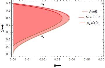
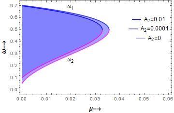
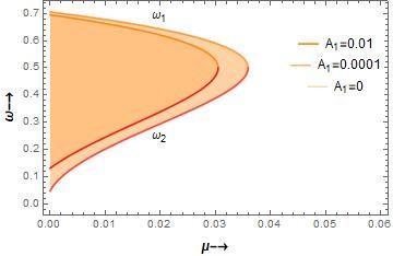
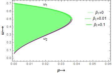
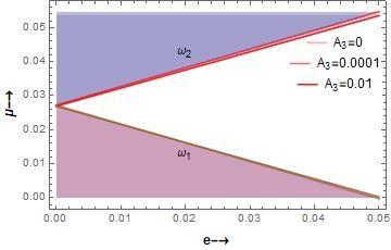
Figures 1-5, shows the correlation between the mass parameter μ and the frequencies $\omega_{1,2}$ varying the various perturbing parameters.
Figure 1. Correlation between $\mu$ and $\omega _ { 1,2 }$ for $A _ { 1 } = A _ { 2 } = 0.001 , \beta _ { 1 } = \beta _ { 2 } = 0 , a = 1$
Figure 2. Correlation between $\mu$ and $\omega _ { 1,2 }$ for $A _ { 1 } = A _ { 3 } = 0.001 , \beta _ { 1 } = \beta _ { 2 } = 0 , a = 1$
Figure 3. Correlation between$\mu$ and $\omega _ { 1,2 }$ for $A _ { 3 } = A _ { 2 } = 0.001 , \beta _ { 1 } = \beta _ { 2 } = 0 , a = 1$
Figure 4. Correlation between$\mu$ and $\omega _ { 1,2 }$ for $A _ { 1 } = A _ { 2 } =A_2= 0.001 , \beta _ { 2 } = 0 .1, a = 1$
Figure 5. Correlation between $\mu$ and $\omega _ { 1,2 }$ for $A _ { 1 } = A _ { 2 } =A_2= 0.001 , \beta _ { 1 } =0 .1, a = 1$
We analyzed the stability of infinitesimal under the elliptical restricted three body problem around the Binary system, where both the primaries are radiating and all the bodies are oblate spheroid as well as the source of radiation, for the small eccentricity ‘’e’’ near the resonance frequency $\omega _ { 2 } = 1 / 2$. We have exploited the method of [19] to investigate the stability of infinitesimal around the triangular equilibrium points and constructed Hamiltonian function, describing the motion of infinitesimal mass in the neighborhoods function of the perturbed system is expanded in the power of the generalized component of momenta up to the second order. We have established a relation for determining the range of stability using simulation techniques by Mathematica software in $\mu - e$ plane. The Hamiltonian function up to the second order of the perturbed system is given as:
$H _ { 2 } = \frac { p _ { 1 + } ^ { 2 } p _ { 2 } ^ { 2 } } { 2 } + p _ { 1 } q _ { 2 } - p _ { 2 } q _ { 1 } + \left[ q _ { 1 } ^ { 2 } \left( \frac { 1 } { 8 } + A \right) - ( K - B ) q _ { 1 } q _ { 2 } - \right.$
$\left. \left( \frac { 5 } { 8 } + \mathrm { C } \right) q _ { 2 } ^ { 2 } \right] + \frac { e \cos f } { 1 + e \cos f } \left[ \left( q _ { 1 } ^ { 2 } \left( \frac { 3 } { 4 } - A \right) + ( K - B ) q _ { 1 } q _ { 2 } + \left( \frac { 9 } { 8 } + \right. \right. \right.$
$\left. \mathrm { C } ) q _ { 2 } ^ { 2 } \right]$ (32)
where,
$\begin{aligned} A = \frac { 7 } { 8 } e ^ { 2 } ( 1 - 2 \mu ) & + \frac { \alpha } { 8 } \left( \frac { 43 } { 32 } - 35 \mu \right) - \frac { 3 } { 4 } \left( 1 - \frac { 7 } { 4 } \mu \right) A _ { 1 } \\ & + \frac { 3 } { 4 } \left( 1 - \frac { 7 } { 4 } \mu \right) A _ { 2 } + \frac { 9 } { 8 } A _ { 3 } \left( 1 - \frac { 7 } { 4 } \mu \right) \\ & + \frac { 1 } { 4 } \beta _ { 1 } ( 1 - 3 \mu ) - \frac { \beta _ { 2 } } { 4 } ( 2 - 3 \mu ) \end{aligned}$
$B = - \frac { 11 } { 4 } e ^ { 2 } \left( 1 - \frac { 20 } { 11 } \mu \right) - \frac { 29 } { 16 } \alpha \left( 1 - \frac { 38 } { 29 } \mu \right) - \frac { 7 } { 2 } A _ { 1 } \left( 1 - \frac { 59 } { 28 } \mu \right) -$
$2 A _ { 2 } \left( 1 - \frac { 29 } { 16 } \mu \right) - \frac { 9 } { 4 } A _ { 3 } \left( 1 - \frac { 5 } { 3 } \mu \right) + \frac { 1 } { 6 } \beta _ { 1 } ( 1 + \mu ) - \frac { \beta _ { 2 } } { 6 } ( 2 - \mu )$
$\mathrm { K } = \frac { 3 } { 4 } \sqrt { 3 } ( 1 - 2 \mu )$ (33)
$\begin{aligned} C = \frac { 1 } { 8 } e ^ { 2 } ( 23 - 22 \mu ) + \frac { \alpha } { 32 } & ( 95 - 220 \mu ) + \frac { 9 } { 4 } A _ { 1 } \left( 1 + \frac { 11 } { 12 } \mu \right) \\ & + \frac { 9 } { 4 } A _ { 2 } \left( 1 - \frac { 11 } { 12 } \mu \right) + \frac { 33 } { 8 } A _ { 3 } ( 1 - \mu ) \\ &\left. + \frac { 1 } { 4 } \beta _ { 1 } ( 1 - \mu ) - \frac { \beta _ { 2 } } { 4 } ( 2 - 3 \mu ) \right) \end{aligned}$
Now considering the canonical transformation $\left[ q _ { 1 } , q _ { 2 } , p _ { 1 } , p _ { 2 } \right]$ which transform into $\left[ q _ { 1 } ^ { \prime } , q _ { 2 } ^ { \prime } , p _ { 1 } ^ { \prime } , p _ { 2 } ^ { \prime } \right]$
$N = \left| \begin{array} { c c c } { a _ { 1 } } & { - a _ { 1 } c _ { 1 } } & { a _ { 1 } \left( 1 - \omega _ { 1 } ^ { 2 } b _ { 1 } \right) } \\ { a _ { 2 } } & { - a _ { 2 } c _ { 2 } } & { a _ { 2 } \left( 1 - \omega _ { 2 } ^ { 2 } b _ { 2 } \right) } \\ { 0 } & { a _ { 1 } \left( 1 - b _ { 1 } \right) } & { a _ { 1 } c _ { 1 } } \end{array} \right|$ (34)
Now using the above canonical transformation, we get:
$q _ { 1 } = a _ { 1 } q _ { 1 } ^ { \prime } + a _ { 2 } q _ { 2 } ^ { \prime }$
$q _ { 2 } = a _ { 1 } c _ { 1 } q _ { 1 } ^ { \prime } + a _ { 2 } c _ { 2 } q _ { 2 } ^ { \prime } + a _ { 1 } b _ { 1 } p _ { 1 } ^ { \prime } - a _ { 2 } b _ { 2 } p _ { 2 } ^ { \prime }$
$p _ { 1 } = - a _ { 1 } c _ { 1 } q _ { 1 } ^ { \prime } - a _ { 2 } c _ { 2 } q _ { 2 } ^ { \prime } + a _ { 1 } \left( 1 - b _ { 1 } \right) p _ { 1 } ^ { \prime } - a _ { 2 } \left( 1 - b _ { 2 } \right) p _ { 2 } ^ { \prime }$ (35)
$p _ { 1 } = a _ { 1 } \left( 1 - w _ { 1 } ^ { 2 } b _ { 1 } \right) q _ { 1 } ^ { \prime } + a _ { 2 } \left( 1 - w _ { 2 } ^ { 2 } b _ { 2 } \right) q _ { 2 } ^ { \prime } + a _ { 1 } c _ { 1 } p _ { 1 } ^ { \prime }$
$- a _ { 2 } c _ { 2 } p _ { 2 } ^ { \prime }$
where,
$l _ { i } = \frac { 9 } { 4 } + 2 c _ { i } + \omega _ { i } ^ { 2 } ; a _ { i } = \frac { 1 } { 2 } \left( \frac { 2 l _ { i } } { \left| \omega _ { i } ^ { 2 } - 1 / 2 \right| } \right) ^ { 1 / 2 } ; b _ { i } = \frac { 1 } { l _ { i } }$
And
$c _ { i } = \frac { - ( K - B ) } { l _ { i } }$ (36)
Now considering $H _ { 2 } = H _ { 2 } ^ { ( a ) } + H _ { 2 } ^ { ( b ) }$,
$H _ { 2 } ^ { ( a ) } =$ Hamiltonian independent of eccentricity.
$H _ { 2 } ^ { ( b ) } =$ Hamiltonian containing the first order approximation in e.
$H _ { 2 } ^ { ( a ) } = \frac { 1 } { 2 } \left( p _ { 1 + } ^ { 2 } p _ { 2 } ^ { 2 } \right) + q _ { 1 } ^ { 2 } \left( \frac { 1 } { 8 } + A \right) - ( K - B ) q _ { 1 } q _ { 2 } - \left( \frac { 5 } { 8 }+c \right)q^2_2$ (37)
Simplifying we get,
$H _ { 2 } ^ { ( b ) } = \frac { e \cos f } { 1 + e \cos f } \left[ \left( \frac { 3 } { 8 } - A \right) a _ { 1 } ^ { 2 } + ( K - B ) a _ { 1 } ^ { 2 } c _ { 1 } + \left( \frac { 9 } { 8 } + \right. \right.$
$\left. \mathrm { c } ) a _ { 1 } ^ { 2 } c _ { 1 } ^ { 2 } \right] q _ { 1 } ^ { \prime 2 } + \left[ \left( \frac { 3 } { 8 } - A \right) a _ { 2 } ^ { 2 } - ( B - K ) a _ { 2 } ^ { 2 } c _ { 2 } + \left( \frac { 9 } { 8 } + \right. \right.$
$\left. C ) c _ { 2 } ^ { 2 } a _ { 2 } ^ { 2 } \right] q _ { 2 } ^ { \prime 2 } + \left[ \left( \frac { 9 } { 8 } + \mathrm { c } \right) a _ { 1 } ^ { 2 } b _ { 1 } ^ { 2 } p _ { 1 } ^ { \prime 2 } + + \left( \frac { 9 } { 8 } + C \right) b _ { 2 } ^ { 2 } a _ { 2 } ^ { 2 } \right] p _ { 2 } ^ { \prime 2 }$
$+ \left[ \left( \frac { 3 } { 8 } - 2 A \right) + ( K - B ) c _ { 2 } - ( K - B ) c _ { 1 } - \left( \frac { 9 } { 8 } + 2 \mathrm { C } \right) c _ { 1 } c _ { 2 } \right] q _ { 1 } ^ { \prime 2 } q _ { 2 } ^ { \prime 2 } + \quad \left[ a _ { 1 } ^ { 2 } b _ { 1 } ( B - K ) + \left( \frac { 9 } { 4 } + 2 C \right) a _ { 1 } ^ { 2 } c _ { 1 } b _ { 1 } \right] q _ { 1 } ^ { \prime } p _ { 1 } ^ { \prime } + [ ( B -$
$\left. K ) a _ { 1 } a _ { 2 } b _ { 1 } + \left( \frac { 9 } { 4 } + 2 C \right) c _ { 2 } a _ { 1 } a _ { 2 } b _ { 1 } \right] q _ { 2 } ^ { \prime } p _ { 1 } ^ { \prime } + a _ { 1 } a _ { 2 } b _ { 1 } ( B - K ) - \left( \frac { 9 } { 4 } + 2 C \right) a _ { 1 } a _ { 2 } c _ { 1 } b _ { 2 } ^ { \prime } p _ { 2 } ^ { \prime }$
$+ \left[ ( B - K ) a _ { 2 } ^ { 2 } b _ { 2 } - \left( \frac { 9 } { 4 } + 2 C \right) a _ { 2 } ^ { 2 } b _ { 2 } c _ { 2 } \right] q _ { 2 } ^ { \prime } p _ { 2 } ^ { \prime } + \left[ a _ { 2 } ^ { 2 } b _ { 2 } ( B - K ) - \left( \frac { 9 } { 4 } + 2 C \right) a _ { 2 } ^ { 2 } c _ { 2 } b _ { 2 } \right] q _ { 2 } ^ { \prime } p _ { 2 } ^ { \prime } - \left( \frac { 9 } { 4 } + 2 C \right) a _ { 1 } a _ { 2 } b _ { 1 } b _ { 2 } p _ { 2 } ^ { \prime } p _ { 1 } ^ { \prime }$ $\left.+ \left[ a _ { 1 } a _ { 2 } b _ { 2 } ( B - K ) - \left( \frac { 9 } { 4 } + 2 C \right) a _ { 1 } a _ { 2 } c _ { 1 } b _ { 2 } \right] q _ { 1 } ^ { \prime } p _ { 2 } ^ { \prime } \right]$ (39)
The characteristic equation is represented as:
$\lambda ^ { 4 } - \left( A ^ { * } + C ^ { * } - 4 \right) \lambda ^ { 2 } + A ^ { * } C ^ { * } - B ^ { * 2 } = 0$ (40)
Let $\lambda _ { 1 } = i \omega _ { 1 }$ and $\cdot \lambda _ { 2 } = i \omega _ { 2 }$. Hence, we get
$\omega ^ { 4 } + \left( A ^ { * } + C ^ { * } - 4 \right) \omega ^ { 2 } + A ^ { * } C ^ { * } - B ^ { * 2 } = 0$
Hence, we get:
$H _ { 2 } ^ { ( b ) } = \frac { e \cos f } { 1 + e \cos f } \left[ a q _ { 2 } ^ { \prime 2 } + b p _ { 2 } ^ { \prime 2 } + c p _ { 2 } ^ { \prime } q _ { 2 } ^ { \prime } + \cdots \right]$ (41)
where, higher order terms in $p _ { 1 } ^ { \prime }$and$q _ { 1 } ^ { \prime }$ are neglected.
Substituting the values of $H _ { 2 } ^ { ( a ) }$ and $H _ { 2 } ^ { ( b ) }$ the normalized Hamiltonian function becomes:
$H _ { 2 } = \frac { 1 } { 2 } \left( p _ { 1 } ^ { \prime 2 } + \omega _ { 1 } ^ { 2 } q _ { 1 } ^ { \prime 2 } \right) - \frac { 1 } { 2 } \left( p _ { 2 } ^ { \prime 2 } + \omega _ { 2 } ^ { 2 } q _ { 2 } ^ { \prime 2 } \right) + e \cos f \left[ a q _ { 2 } ^ { \prime 2 } + \right.$
$\left. b p _ { 2 } ^ { \prime 2 } + c p _ { 2 } ^ { \prime } q _ { 2 } ^ { \prime } + \cdots \right]$ (42)
where,
$a = \left( \frac { 3 } { 8 } - A \right) a _ { 1 } ^ { 2 } + ( K - B ) a _ { 1 } ^ { 2 } c _ { 1 } + \left( \frac { 9 } { 8 } + \mathrm { C } \right) a _ { 1 } ^ { 2 } c _ { 1 } ^ { 2 }$
$b = \left( \frac { 9 } { 8 } + C \right) a _ { 1 } ^ { 2 } b _ { 1 } ^ { 2 }$
$c = \left\{ - ( K - B ) a _ { 2 } ^ { 2 } b _ { 2 } - \left( \frac { 9 } { 8 } - \mathrm { C } \right) 2 a _ { 1 } ^ { 2 } b _ { 2 } c _ { 2 } \right\}$ (43)
We introduction the transformation of the variables, which are given as:
$q _ { 1 } ^ { \prime } = \frac { \sqrt { 2 \alpha _ { 1 } } } { \omega _ { 1 } } \sin \omega _ { 1 } \left( f + \gamma _ { 1 } \right)$
$q _ { 2 } ^ { \prime } = \frac { \sqrt { 2 \alpha _ { 2 } } } { \omega _ { 2 } } \sin \omega _ { 2 } \left( f - \gamma _ { 2 } \right)$
$p _ { 1 } ^ { \prime } = \sqrt { 2 \alpha _ { 1 } } \cos \omega _ { 1 } \left( f + \gamma _ { 1 } \right)$
$p _ { 2 } ^ { \prime } = \sqrt { 2 \alpha _ { 1 } } \cos \omega _ { 2 } \left( f - \gamma _ { 2 } \right)$ (44)
The perturbation in Hamiltonian is represented as follows:
$H = \frac { e \cos f } { 1 + e \cos f } \left[ a q _ { 2 } ^ { \prime 2 } + b p _ { 2 } ^ { \prime 2 } + c p _ { 2 } ^ { \prime } q _ { 2 } ^ { \prime } + \cdots \right]$ (45)
From the equation (44) and (45)
$H = \frac { e \cos f } { 1 + e \cos f } \left[ \frac { 2 a \alpha _ { 2 } } { \omega _ { 2 } ^ { 2 } } \sin ^ { 2 } \omega _ { 2 } \left( f - \gamma _ { 2 } \right) + 2 b \alpha _ { 2 } \cos ^ { 2 } \omega _ { 2 } \left( f - \gamma _ { 2 } \right) - \frac { c \alpha _ { 2 } } { w _ { 2 } } \sin \omega _ { 2 } 2 \left( f - \gamma _ { 2 } \right) \right]$ (46)
where,
$\omega _ { 2 } = \frac { 1 + 2 \epsilon _ { 1 } } { 2 } \quad \left( \epsilon _ { 1 } \leq 1 \right)$ (47)
Using equations (46), (47) and taking the average of the terms with finite frequencies in the range 0 to 2π, the Hamiltonian H2 is reduced to the form.
$H _ { 2 } = e \left[ U \cos \left( 2 \epsilon _ { 1 } f - 2 \omega _ { 2 } \gamma _ { 2 } \right) + V \sin \left( 2 \epsilon _ { 1 } f - 2 \omega _ { 2 } \gamma _ { 2 } \right) \right] \alpha _ { 2 }$ (48)
where, $U = \frac { ( b - 4 a ) } { 2 } , V = c$.
Now introducing the canonical transformation as:
$\overline { \alpha _ { 1 } } = \alpha _ { 1 } ; \overline { \gamma _ { 1 } } = \gamma _ { 1 } ; \overline { \alpha _ { 2 } } = \alpha _ { 2 } ; \overline { \gamma _ { 2 } } = \gamma _ { 2 } - 2 \epsilon _ { 1 } f$ (49)
Also, assuming $\overline { H }$ be the transformed form of Hamiltonian H in the new variables, then we have:
$\begin{aligned} d F \left( q _ { i } , \overline { q } _ { t } , t \right) = & \sum \overline { p } _ { p } \overline { d } q _ { i } - \sum p _ { i } d q _ { i } + ( \overline { H } - H ) d t \\ d F \left( q _ { i } , \overline { q } _ { i } V \right) = & \overline { \gamma } _ { 1 } d \overline { \alpha } _ { 1 } - \overline { \gamma } _ { 2 } d \overline { \alpha } _ { 2 } - \gamma _ { 1 } d \alpha _ { 1 } - \gamma _ { 2 } d \alpha _ { 2 } + ( \overline { H } \\ - H ) d f \end{aligned}$
That is we get
$\begin{aligned} ( \overline { H } - H ) d f - 2 \epsilon _ { 1 } f d \alpha _ { 2 } = & \frac { \partial F } { \partial \alpha _ { 1 } } d \alpha _ { 1 } + \frac { \partial F } { \partial \alpha _ { 2 } } d \alpha _ { 2 } + \frac { \partial F } { \partial \overline { \alpha _ { 1 } } } d \overline { \alpha _ { 1 } } + \\ & \frac { \partial F } { \partial \overline { \alpha _ { 2 } } } d \overline { \alpha _ { 2 } } + \frac { \partial F } { \partial f } d f \end{aligned}$ (50)
Equating the coefficients of the $d \alpha _ { 2 }$ and $d f$ from both sided, we obtained:
$\overline { H } - H = \frac { \partial F } { \partial f } ; - 2 \epsilon _ { 1 } f = \frac { \partial F } { \partial \alpha _ { 2 } } ; F = F ( \alpha , V )$ (51)
$d F = \frac { \partial F } { \partial \alpha _ { 2 } } d \alpha _ { 2 } + \frac { \partial F } { \partial f } d f ; \frac { d F } { d \alpha _ { 2 } } = \frac { \partial F } { \partial \alpha _ { 2 } } = - 2 \epsilon _ { 1 } f$
That is
$F = - 2 \epsilon _ { 1 } f \alpha _ { 2 }$ (52)
Hence,
$\overline { H } = H - 2 \epsilon _ { 1 } \alpha _ { 2 }$ (53)
From equation (48) and (53), considering the non periodic part of the perturbation i.e.terms independent from true anomaly υ, we have:
$\overline { H _ { 2 } } = e \left[ U \cos 2 w _ { 2 } \overline { \gamma _ { 2 } } - V \sin 2 w _ { 2 } \overline { \gamma _ { 2 } } \right] \overline { \alpha _ { 2 } } - 2 \epsilon _ { 1 } \overline { \alpha _ { 2 } }$ (54)
where,
$U = \frac { ( b - 4 a ) } { 2 }$ and $V = c$ (55)
The transformed Hamiltonian $\overline { H _ { 2 } }$ given by (54) is now independent of f. Let the integral be:
$\overline { H _ { 2 } } = h _ { 1 } =$ constant (56)
Therefore, from (54) we obtain:
$e \left[ U \cos 2 w _ { 2 } \overline { \gamma _ { 2 } } - V \sin 2 w _ { 2 } \overline { \gamma _ { 2 } } \right] \overline { \alpha _ { 2 } } - 2 \epsilon _ { 1 } \overline { \alpha _ { 2 } } = h _ { 1 }$ (57)
Replacing,
$\cos \theta = U / \sqrt { \left( U ^ { 2 } + V ^ { 2 } \right) } , \sin \theta = V / \sqrt { \left( U ^ { 2 } + V ^ { 2 } \right) }$ (58)
Using (57), the above expression (58) gets reduced to the following form:
$e \cos \left( 2 w _ { 2 } \overline { \gamma _ { 2 } } + \theta \right) = \left[ h + \frac { 2 \epsilon _ { 1 } } { e \sqrt { \left( U ^ { 2 } + V ^ { 2 } \right) } } \overline { \alpha _ { 2 } } \right] / \overline { \alpha _ { 2 } }$ (59)
where, $h = \frac { h _ { 1 } } { e \sqrt { \left( U ^ { 2 } + V ^ { 2 } \right) } }$.
Therefore, the motion with Hamiltonian $\overline { H _ { 2 } }$ is given by (55), (56) and (59), possessing the integral is represented as follows:
$\overline { H _ { 2 } } = e \sqrt { \left( U ^ { 2 } + V ^ { 2 } \right) } h$
where,
$\cos \left( 2 \omega _ { 2 } \overline { \gamma _ { 2 } } + \theta \right) = \left[ h + \frac { 2 \epsilon _ { 1 } } { e \sqrt { \left( U ^ { 2 } + V ^ { 2 } \right) } } \overline { \alpha _ { 2 } } \right] / \overline { \alpha _ { 2 } }$ (60)
θ is determined by the relation (58). Solving (59), we obtain;
$\overline { \alpha _ { 2 } } \cos \left( 2 \omega _ { 2 } \overline { \gamma _ { 2 } } + \theta \right) = h + \frac { 2 \epsilon _ { 1 } } { e \sqrt { \left( U ^ { 2 } + V ^ { 2 } \right) } } \overline { \alpha _ { 2 } }$
$\overline { \alpha _ { 2 } } = \mathrm { h } / \left[ \cos \left( 2 \omega _ { 2 } \overline { \gamma _ { 2 } } + \theta \right) - \frac { 2 \epsilon _ { 1 } } { e \sqrt { \left( U ^ { 2 } + V ^ { 2 } \right) } } \right]$
The parameter $\overline { \alpha _ { 2 } }$will be unbounded if:
$\frac { 2 \epsilon _ { 1 } } { e \sqrt { \left( U ^ { 2 } + V ^ { 2 } \right) } } | < 1 ;$ or $\left| \epsilon _ { 1 } \right| < ( e \sqrt { \left( U ^ { 2 } + V ^ { 2 } \right) } ) / 2$ (61)
The inequality (61) determines the region of the parametric resonance in the ($\mu - e$) plane in the neighborhood of equilibrium points corresponding to $\omega _ { 2 } = 1 / 2$ which is given as:
$\mu _ { 0 } = 0.0285955 - 0.00654729 \left( \beta _ { 1 } + \beta _ { 2 } \right) - 0.0523783 \alpha -$
$0.112941 A _ { 1 } - 0.063836 A _ { 2 } - 0.0294628 A _ { 3 }$ (62)
In the neighborhood of μ0, let us take;
$\mu = \mu _ { 0 } + h$ so that $\mu - \mu _ { 0 } = h$
Now expanding ω2(μ) by Taylor’s theorem, we get;
$\omega _ { 2 } ( \mu ) = \omega _ { 2 } \left( \mu _ { 0 } + h \right) = \omega _ { 2 } \left( \mu _ { 0 } \right) + h \left[ d \omega _ { 2 } ( \mu ) / d \mu \right] _ { \mu = \mu _ { 0 } }$
That is $\epsilon _ { 1 } = \left( \mu - \mu _ { 0 } \right) \cdot \left[ d \omega _ { 2 } ( \mu ) / d \mu \right] _ { \mu = \mu _ { 0 } }$
Now using equation (61), the region of parametric resonance is expressed as:
$\left| \left( \mu - \mu _ { 0 } \right) \right| < \frac { e \left( U ^ { 2 } + V ^ { 2 } \right) ^ { 1 / 2 } } { 2 } \left[ d w _ { 2 } ( \mu ) / d \mu \right] _ { \mu = \mu _ { 0 } } < e B _ { 1 i }$ (63)
where,
$B _ { 1 } = \frac { \sqrt { \left( U ^ { 2 } + V ^ { 2 } \right) } } { 2 } \left[ d w _ { 2 } ( \mu ) / d \mu \right] _ { \mu = \mu _ { 0 } }$ (64)
Hence, the region of existence of parametric resonance is determined by the following inequality:
$\mu _ { 0 } - e B _ { 1 } < \mu < \mu _ { 0 } + e B _ { 1 }$ (65)
we have at $\omega _ { 2 } = 1 / 2$
$\left| \omega _ { 2 } ^ { 2 } - \frac { 1 } { 2 } \right| = \frac { 1 } { 4 }$
Hence,
$\mu ^ { 2 } - \mu + \frac { 1 } { 27 } \left[ 1 - \frac { 2 } { 9 } \beta _ { 1 } - \frac { 2 } { 9 } \beta _ { 2 } - \frac { 94 } { 9 } \alpha - \frac { 119 } { 6 } A _ { 1 } - \frac { 61 } { 6 } A _ { 2 } \right.$
$\left. - 17 A _ { 3 } \right] = 0$
Solving the above equation as a quadratic in μ, we get
$\mu = \frac { 1 } { 2 } \pm \frac { 1 } { 6 } \sqrt { \frac { 23 } { 13 } } \left[ 1 - \frac { 4 } { 207 } \beta _ { 1 } + \frac { 2 } { 9 } \beta _ { 2 } + \frac { 188 } { 207 } \alpha + \frac { 119 } { 69 } A _ { 1 } + \right.$
$\left. \frac { 61 } { 69 } A _ { 2 } + \frac { 34 } { 23 } A _ { 3 } \right]$
Taking the negative sign, we get
$\begin{aligned} \mu = 0.0285955 & - 0.00654729 \left( \beta _ { 1 } + \beta _ { 2 } \right) - 0.0523783 \alpha \\ & - 0.112941 A _ { 1 } - 0.063836 A _ { 2 } \\ & - 0.0294628 A _ { 3 } \end{aligned}$
Hence from equation (64), we get
$B _ { 1 } = 0.05641678587652361 - 2.0692243397659893 \mathrm { Al }$
$- 0.676545253188928 \mathrm { A } 2$
$- 1.7314172901066136 \mathrm { A } 3$
$- 0.9425222140171992 \alpha$
$- 0.014794126415526613 \beta _ { 1 }$
$- 0.010493306202522411 \beta _ { 2 }$
Hence the boundary of the region obtained by (64) of the parametric resonance about $\omega _ { 2 } = 1 / 2$ in the first approximation in e is given by:
$\begin{aligned} \mu = 0.0285955 & - 0.00654729 \left( \beta _ { 1 } + \beta _ { 2 } \right) - 0.0523783 \alpha \\ & - 0.112941 \mathrm { A } 1 - 0.063836 \mathrm { A } 2 \\ & - 0.0294628 \mathrm { A } 3 \\ & \pm \mathrm { e } ( 0.05641678587652361 \\ & - 2.0692243397659893 \mathrm { A } 1 \\ & - 0.676545253188928 \mathrm { A } 2 \\ & - 1.7314172901066136 \mathrm { A } 3 \\ & - 0.9425222140171992 \alpha \\ & - 0.014794126415526613 \beta _ { 1 } \\ &\left. - 0.01049330620252241 \beta _ { 2 } \right) \end{aligned}$
Figure 6. Bifurcation of μ-e plane into stable and unstable regions for $A _ { 1 } = A _ { 2 } = 0.001 , \beta _ { 1 } = \beta _ { 2 } = 0.1 , a = 1$
Figure 7. Bifurcation of μ-e plane into stable and unstable regions for $A _ { 1 } = A _ { 3 } = 0.001 , \beta _ { 1 } = \beta _ { 2 } = 0.1 , a = 1$
Figure 8. Bifurcation of μ-e plane into stable and unstable regions for $A _ { 3 } = A _ { 2 } = 0.001 , \beta _ { 1 } = \beta _ { 2 } = 0.1 , a = 1$
Figure 9. Bifurcation of μ-e plane into stable and unstable regions for $A _ { 1 } = A _ { 2 } =A_3= 0.001 , \beta _ { 2 } = 0.1 , a = 1$
Figure 10. Bifurcation of μ-e plane into stable and unstable regions for $A _ { 1 } = A _ { 2 } =A_3= 0.001 , \beta _ { 1 } = 0.1 , a = 1$
Now the stability of the triangular equilibrium points is analyzed by using the simulation techniques with Mathematica software. The plots in the μ-e plane as a function of the different perturbing factors are plotted and the bifurcation of the plane into stable and unstable region is shown in Figures 6-10.
The stability of infinitesimal around the triangular equilibrium points under the elliptical restricted three body problem has been discussed, when all the participating bodies are oblate spheroid and the primaries are the source of radiation. The effect of the oblateness and radiation pressure effect the location and resonance stability of triangular equilibrium points of the elliptical restricted three body problem in particular case when e=0 at and near the resonance frequency ω2=1/2, which is analyzed from the graphical behavior of the triangular equilibrium points. In circular case near the resonance frequency, we have constructed a suitable normalization convergent Hamiltonian function and investigated the stability analytically and numerically due to oblateness and radiation of primaries up to the second order terms. The region of stability in the μ-ω plane has been clearly marked as shown in figures 1-5. As observed from the figures the stable region decreases with increase in the value of oblateness factor as well as radiation factor. However, the decrease is more prominent for the change in the value of the oblateness factors.
We have investigated the stability of infinitesimal mass in the model of elliptical restricted three body problem as well near the resonance frequency ω2=1/2. The method used by [10] has been adopted to investigate the stability of infinitesimal around the triangular equilibrium points. The Hamiltonian function of the perturbed system is expanded in the power of the generalized component of moments up to the second order. We have established a relation in μ-e plane for determining the range of stability using simulation techniques with the help of mathematical software Mathematica 10. The region of stability of the linear problem in μ-e plane has been plotted and stable and unstable region has been separated as shown in figures 6-10. The shaded region in the graphs shows the region of stability. From the plots, we observe that the region of stability, in the elliptic case, decreases very slightly with the increase in the values of the parameters: oblateness and radiation pressure.
The financial assistance from Chattisgarh Council of Science and Technology (Endt. no.2260/CCOST/MRP/2015) is duly acknowledged with gratitude B.
[1] Markeev, A.P. (2005). On one special case of parametric resonance problem of celestical mechanics. Astronomy Letters, 31(5): 350-356. https://doi.org/10.1134/1.1922534
[2] Danby, J.M.A. (1964). Stability of the triangular points in the elliptic restricted problem of three bodies. Astronomical Journal, 69: 165-172. https://doi.org/10.1086/109254
[3] Bennett, A. (1965). Characteristic exponents of the five equilibrium solutions in the elliptically restricted problem. Icarus, 4(2): 177-189. https://doi.org/10.1016/0019-1035(65)90060-6
[4] Narayan, A., Ramesh, C. (2011). Effect of photo gravitation and oblateness and the triangular Lagrangian points in elliptic restricted three body problem. International Journal of Pure and Applied Mathematics, 68(2): 201-224.
[5] Kumar, C.R., Narayan, A. (2012). Existance and stability of collinear equilibrium points in elliptical restricted three body problem under the effects of photogravitational and oblateness primaries. International Journal of Pure and Applied Mathematics, 80(4): 477-494.
[6] Narayan, A., Singh, N. (2014). Existence and stability of collinear equilibrium points in elliptical restricted three body problem under the radiating primaries. Astrophysics and Space Science, 354(2): 355-368. https://doi.org/10.1007/s10509-014-2094-5
[7] Narayan, A., Singh, N. (2014). Motion and stability of triangular equilibrium points in elliptical restricted three body problem under the radiating primaries. Astrophysics and Space Science, 352(1): 57-70. https://doi.org/10.1007/s10509-014-1903-1
[8] Usha, T., Narayan, A., Ishwar, B. (2014). Effects of radiation and triaxiality of primaries on triangular equilibrium points in elliptic restricted three body problem. Astrophs, Space Sci., 349(1): 151-164. https://doi.org/10.1007/s10509-013-1655-3
[9] Usha, T., Narayan, A. (2016). Linear stability and resonance of triangular equilibrium points in elliptic restricted three body problem with radiating primary and triaxial secondary. International Journal of Advanced Astronomy, 4(2): 82. https://doi.org/10.14419/ijaa.v4i2.6536
[10] Khasan, S. (1990). Liberation solution to the photogravitational restricted three body problem. Cosmic Research, 34(2): 146-151.
[11] Singh, J., Aishetu, U. (2012). Motion in the photogravitational elliptic restricted three body problem under an oblate primary. The Astrnomical Journal, 143(5): 109. https://doi.org/10.1088/0004-6256/143/5/109
[12] Singh, J., Aishetu, U. (2012). On the stability of triangular points in the elliptic R3BP under radiating and oblate primaries. Astrophsics and Space Science, 341(2): 349-358. https://doi.org/10.1007/s10509-012-1109-3
[13] Conxita, P. (1995). Ejection collision orbits with the move massive primary in the planar elliptic restricted three body problem. Celestial Mechanics and Dynamical Astronomy, 61(4): 315-331. https://doi.org/10.1007/BF00049513
[14] Hallan, P., Rana, N. (2001). The existence and stability of equilibrium points in the Robe’s restricted three body problem. Celestial Mechanics and Dynamical Astronomy, 79(2): 145-155. https://doi.org/10.1023/A:1011173320720
[15] Şelaru, D., Cucu–Dumitrescu, C. (1995). Infinitesimal orbit around Lagrange points in the elliptic restricted three body problem. Celestial Mechanics and Dynamical Astronomy, 61(4): 333-346. https://doi.org/10.1007/BF00049514
[16] Şelaru, D., Cucu–Dumitrescu, C. (1994). An analytic asymptotical solution in the three body problem. Romanian Astronomical Journal, 4(1): 59-67.
[17] Floria, L. (2004). On an analytical solution in the planar elliptical restricted three body problem. Monografsem. Mat. Garacia de Galdeano, 31: 135-144.
[18] Subba Rao, P.V., Sharma, R.K. (1996). Effect of oblatenes on the non-linear stability of L_4 in the restricted three body problem. Celestial Mechanics and Dynamical Astronomy, 65(3): 291-312. https://doi.org/10.1007/BF00053510
[19] Markeev, A.P. (1978). Libration points in celestial mechanics and astro dynamics. Moscow Izdate Nauka, 1: 1.