Fayza Boussekra | Abdessalam Makouf
OPEN ACCESS
This paper proposes a new speed and position sensorless control method of Interior permanent magnet synchronous motors (IPMSM) using sliding mode observer based on Active Flux concept. First, a new description of IPMSM dynamic model in the stationary reference frame using active flux concept is proposed. The model obtained suits for both SPMSM and IPMSM in the stationary reference frame, Therefore, all that sensorless controls proposed for SPMSM can be directly and easily applied to IPMSM. Secondly, from the measurement of the voltages and the currents, a new analysis of the observability property is developed. Then, the sliding mode observer (SMO) structure and its design method are described in the stationary reference frame by using the active flux equation. A “chattering” phenomenon is reduced by using this technique. The stability of the proposed SMO was verified using the Lyapunov function. The speed and position of the IPMSM are estimated based on back EMF which are related to the active flux. Moreover, the zero d-axis current control strategy is used to control the IPMSM. Finally, the proposed method on the proposed model has been simulated and tested to show the effectiveness of the proposed scheme.
active flux, Interior permanent magnet synchronous motor, Sensorless control, Sliding mode observer
The importance of high efficiency at low speed and high torque/power density make many industrial applications using permanent magnets synchronous motors (PMSM), especially interior permanent magnet synchronous motors (IPMSM) because it has many advantages compared to the other types of motors in efficiency and power density [1-3].
For feedback control, the knowledge of position and rotor speed are necessary. Thus, speed sensors such as the encoders or the resolvers are utilized. In order to reduce the motor size, the hardware complexity, cost, and to improve robustness and reliability of the drive system the sensorless vector control of IPMSM has been proposed [4-6].
Two approaches of sensorless control of IPMSM can be cited. The first approach uses the excitation at high frequency to detect saliency difference between direct axis-d and quadrature axis-q. This method gives good performances at low speeds range but increase the complexity of sensorless control system and induces undesirable effects on the motor performances as the increasing of losses [7-9]. The second approach using the estimation of the back EMF value deduced from the integration of the total flux linkage on the stator phase circuits is simple. This approach is very adapted for the IPMSM drive system allowing to achieve good performances at medium and high speeds operating region [10-12]. However, these methods can fail at very low and zero rotating speed since the IPMSM dynamic model is quite complex, nonlinear, coupled and also the parameters are most often not known exactly during operating system [13]. To enhance the performance of the sensorless operation at low speed, several sensorless control methods has been developed. Online parameter estimation method is introduced by Chen [4]. It consists to minimize the effects of parameter variations using a new IPMSM mathematical model, in [14] a robust sensorless control with respect to the inverter irregularities, using of an on-line stator resistance identification method is proposed. the authors propose by Inoue et al. [15] a sensorless-control method based on the extended (EMF) concept for improving performance such as the operating speed range and the accuracy of position estimation.
Therefore, in order to simplify the IPMSM dynamic model and also make it more accessible to automated design technique. For instance, the concept of extended back-electromotive force (EMF) has been introduced by Chen et al. [16]. Indeed, it was the first attempt that has developed a new mathematical model for PMSM, suitable for both SPMSM and IPMSM and also valid for Reluctance Synchronous Motors (RSM). For the same purpose, Boldea et al. [17] propose a simple and efficient model of IPMSM based on the active flux concept. Using this concept, the IPMSM dynamic model can be described as an SPMSM model in the stationary reference frame (α, β) and also, makes it accessible for control design. The “active flux” concept which “turns all salient-pole rotor AC machines into fictitious non-salient-pole machines” is defined as the torque-producing virtual flux which multiplies the iq current component on the d axis in the electromagnetic torque equation of ac machines in the rotating reference frame (d, q).
Another approach that can be taken to simplify the model of IPMSM called a fictitious permanent-magnet flux concept which was proposed by Koonlaboon [18]. Actually, there is no difference between the concept of fictitious permanent-magnet flux, the extended EMF and the active flux approach. However; using fictitious flux, the IPMSM dynamics model can suit the sensorless control scheme but not all the available control schemes.
Recently, and not far from the previous approaches, a new proposition to simplify and unify the AC model is introduced by Koteich et al. [19]. In fact it is a generalization of all the previous concepts, such as the extended EMF, the active flux and the fictitious flux concept. This approach is called the equivalent flux.
On the other hand, to improve both accuracy and robustness of rotor speed and position estimations, sliding mode observer (SMO) design is developed. The sliding mode technique is one of the important and famous nonlinear control method, thanks to the inherent robustness properties and its simplicity. The "chattering effect" it's the main disadvantage of this techniques which can be reduced, generally, by using the low pass filter [20-23].
In this paper a new sensorless vector control of IPMSM is proposed. The rotor speed and rotor position are estimated from back EMF estimation with sliding mode observer (SMO) based on active flux concept. The objective is to estimate easily and rapidly the both rotor position and speed of the motor in wide speed range. The main contributions of this work are as follows: Firstly, a new and simple description of IPMSM dynamic model in the stationary reference frame based on an "Active Flux" concept is proposed. The model obtained suits for both SPMSM and IPMSM, Therefore, all that sensorless controls proposed for SPMSM can be directly and easily applied to IPMSM. Secondly, from the measurement of the voltages and the currents, a new analysis of the observability property in the (α, β) coordinate by using the “Active Flux” concept is proposed. Then, a sliding mode observer is designed on the stationary reference frame by using the active flux appraoch. A “chattering” phenomenon is reduced by using this technique. The stability of the proposed SMO was verified using the Lyapunov function. Moreover, the zero d-axis current control strategy is used to control the IPMSM. Finally, the proposed method on the proposed model has been simulated and tested to show the effectiveness of the proposed scheme.
This paper is organized as follows: the next section exposes the concept of the active flux. the section 3 present new description dynamical model of IPMSM in the (α, β) frame. An analysis of the IPMSM observability is presented in Section 4. In section 5 a sliding mode observer is designed in the stationary reference frame by using the active flux appraoch to estimate both rotor position and speed in wide speed range. This section discusses the stability of the error system by Lyapunov approach. Finally, the simulation results are presented in section 6 to validate the theoretical description and show the feasibility of the proposed method.
In this part, a new mathematical model of IPMSM is proposed by using the flux active concept.
2.1 Active flux concept
To understand the "Active Flux" term, we need to define the electromagnetic torque equation of IPMSM in (d,q) reference frame. The electromagnetic torque can be expressed as:
$T_{e}=\frac{3}{2} P\left(\phi_{f}+\left(L_{d}-L_{q}\right) i_{d}\right) i_{q}$ (1)
where, P is the number of pole pairs, ϕf is the rotor flux, Ld and Lq are d-axis and q-axis inductances, and id, iq are the d-q axes stator currents respectively.
Let us now define the active flux ϕa as:
$\phi_{a}=\phi_{f}+\left(L_{d}-L_{q}\right) i_{d}$ (2)
For SPMSM: Ld=Lq, ϕa=ϕf
For IPMSM: Ld≠Lq, ϕa=ϕf+(Ld-Lq)id
From equation (2), the active flux vector has the same direction with the real rotor flux vector and the d-axis current. So, the required rotor position can be obtained from its estimate in the same way as is done for the SPMSM [24].
According to (1) and (2) the expression of the torque T_e in the rotor reference frame can be described by the following equation:
$T_{e}=\frac{3}{2} P \phi_{a} i_{q}$ (3)
So, the active flux which “turns all salient-pole rotor AC machines into fictitious non-salient-pole machines” is defined as the torque producing virtual flux which multiplies the iq current component on the d axis in the electromagnetic torque equation of AC machines in the d-q reference frame [17].
Figure 1. Vector diagram of active flux in (d, q) reference frame
According to (3), it appears the linear form of torque which can be controlled directly by $i_{q}$ when $\phi_{a}$ is fixed.
The voltage vector equation is given by:
$\bar{u}_{s}=R \bar{\imath}_{s}+\frac{d \bar{\phi}_{s}}{d t}$ (4)
where, us is stator voltage, iS is the stator current, R is the stator resistance, ϕs is the stator flux
According to (4), the stator flux is:
$\bar{\phi}_{s}=\int\left(\bar{u}_{s}-R \bar{\imath}_{s}\right) d t$ (5)
In the rotor reference frame (d, q), the stator flux can be described by
$\bar{\phi}_{s}=\phi_{d}+j \phi_{q}$ (6)
where,
$\left\{\begin{array}{l}\phi_{d}=\phi_{f}+L_{d} i_{d} \\ \phi_{q}=L_{q} i_{q}\end{array}\right.$ (7)
Further, the active flux vector can be rewritten as:
$\bar{\phi}_{a}=\phi_{f}+\left(L_{d}-L_{q}\right) i_{d}+j L_{q} i_{q}-j L_{q} i_{q}$ (8)
After little arrangements we can write:
$\bar{\phi}_{a}=\phi_{f}+L_{d} i_{d}+j L_{q} i_{q}-L_{q}\left(i_{d}+j i_{q}\right)$ (9)
Then, the active flux is given as:
$\bar{\phi}_{a}=\bar{\phi}_{s}-L_{q} i_{s}$ (10)
where,
$\bar{i}_{s}=i_{d}+j i_{q}$ (11)
The Eq. (10) create a simple relationship between active flux and stator flux and shows that the q-axis inductance L_q is the only motor parameters affected.
Substituting stator flux estimation Eq. (5) into active flux Eq. (10) we obtain:
$\bar{\phi}_{a}=\int\left(\bar{u}_{s}-R \bar{\imath}_{s}\right) d t-L_{q} \bar{l}_{s}$ (12)
2.2 Design of IPMSM model using the active flux
The mathematical model of the IPMSM is established from the fluxes components ϕaα and ϕaβ which are defined in the reference frame (α, β) as:
$\left\{\begin{array}{l}\phi_{a \alpha}=\int\left(u_{\alpha}-R i_{\alpha}\right) d t-L_{q} i_{\alpha} \\ \phi_{a \beta}=\int\left(u_{\beta}-R i_{\beta}\right) d t-L_{q} i_{\beta}\end{array}\right.$ (13)
where, (uα, uβ) is the voltage on the fixed coordinate, and (i_α, i_β) is the current on the fixed coordinate.
The derivative of Eq. (13) gives:
$\left\{ \begin{align} & \frac{d{{i}_{\alpha }}}{dt}=-\frac{R}{{{L}_{q}}}{{i}_{\alpha }}+\frac{{{u}_{\alpha }}}{{{L}_{q}}}-\frac{1}{L{}_{q}}\frac{d{{\phi }_{a\alpha }}}{dt} \\ & \frac{d{{i}_{\beta }}}{dt}=-\frac{R}{{{L}_{q}}}{{i}_{\beta }}+\frac{{{u}_{\beta }}}{{{L}_{q}}}-\frac{1}{L{}_{q}}\frac{d{{\phi }_{a\beta }}}{dt} \\\end{align} \right.$ (14)
According to Figure $1,$ the fluxes components $\phi_{a \alpha}$ and $\phi_{a \beta}$ can be written as:
$\left\{\begin{array}{l}\phi_{a \alpha}=\phi_{a} \cos \theta \\ \phi_{a \beta}=\phi_{a} \sin \theta\end{array}\right.$ (15)
Using (15), the Eq. (14) can be rewritten as follows:
$\left\{ \begin{align} & \frac{d{{i}_{\alpha }}}{dt}=-\frac{R}{{{L}_{q}}}{{i}_{\alpha }}+\frac{{{u}_{\alpha }}}{{{L}_{q}}}-\frac{1}{L{}_{q}}\frac{d{{\phi }_{a}}}{dt}\cos \theta +\frac{1}{{{L}_{q}}}{{\phi }_{a}}P{{\omega }_{r}}\sin \theta \\ & \frac{d{{i}_{\beta }}}{dt}=-\frac{R}{{{L}_{q}}}{{i}_{\beta }}+\frac{{{u}_{\beta }}}{{{L}_{q}}}-\frac{1}{L{}_{q}}\frac{d{{\phi }_{a}}}{dt}\sin \theta -\frac{1}{{{L}_{q}}}{{\phi }_{a}}P{{\omega }_{r}}\cos \theta \\\end{align} \right.$ (16)
Defining the following variables:
$\left\{ \begin{align} & {{e}_{\alpha }}=-{{\phi }_{a}}P{{\omega }_{r}}\sin \theta \\ & {{e}_{\beta }}={{\phi }_{a}}P{{\omega }_{r}}\cos \theta \\\end{align} \right.$ (17)
where, ${e}_{\alpha}$ and ${e}_{\boldsymbol{\beta}}$ represent the back EMF along $\alpha$ -axis and $\beta$ axis.
The new proposed dynamic model of IPMSM in the stationary reference frame $(\alpha, \beta)$, with taking into account the mechanical dynamic expression, is given by (18):
$\left\{ \begin{align} & \frac{d{{i}_{\alpha }}}{dt}=-\frac{R}{{{L}_{q}}}{{i}_{\alpha }}+\frac{{{u}_{\alpha }}}{{{L}_{q}}}-\frac{1}{{{L}_{q}}}{{e}_{\alpha }}-\frac{1}{L{}_{q}}\frac{d{{\phi }_{a}}}{dt}\cos \theta \\ & \frac{d{{i}_{\beta }}}{dt}=-\frac{R}{{{L}_{q}}}{{i}_{\beta }}+\frac{{{u}_{\beta }}}{{{L}_{q}}}-\frac{1}{{{L}_{q}}}{{e}_{\beta }}-\frac{1}{L{}_{q}}\frac{d{{\phi }_{a}}}{dt}\sin \theta \\ & \frac{d{{\omega }_{r}}}{dt}=\frac{3P}{2J}{{\phi }_{a}}(i_{\beta }^{{}}\cos \theta -{{i}_{\alpha }}\sin \theta )-\frac{f}{J}{{\omega }_{r}}-\frac{{{T}_{l}}}{J} \\\end{align} \right.$ (18)
where, Tl is the load torque, J and f are the moment of inertia of the rotor and friction coefficient, respectively.
The system described in (18) has a simple structure, compared to the classical model given by Chen et al. [16], it suits both SPMSM and IPMSM in the stationary reference frame. The new IPMSM dynamic model based on the active flux concept has the following properties and advantages:
1- The proposed IPMSM dynamic model based on active flux is simpler than the classical model in stationary reference frame and extended EMF dynamic model and also simpler than the fictitious magnet flux model.
2-The new model is independent on motor inductance matrix parameters.
3- The new model shows a great similarity and equivalence between the IPMSM and the SPMSM with the real magnet flux for IPMSM in the (α,β ) coordinate .
4- The sensorless controls proposed for SPMSM can be directly and easily applied to IPMSM.
5-With the new model, the sliding mode observer theory can be applied easily to the IPMSM in (α,β ) coordinate as is done for the SPMSM.
6-The back EMF formula induced by the active flux of IPMSM is exactly the EMF introduced of SPMSM.
In order to design an observer it is necessary to analyse the observability of the system and show under which conditions the IPMSM is observable in the (α,β) coordinate. Several approaches have been presented in literature to study the observability of nonlinear systems. In this section, we study the observability of IPMSM based on local weak observability theory of nonlinear systems which is introduce by Hermann and Krener [25].
3.1 Electromechanical model observability
By using the flux active concept, the mathematic model of IPMSM can be written as follows:
$\left( \begin{align} & {{{\dot{x}}}_{1}} \\ & {{{\dot{x}}}_{2}} \\ & {{{\dot{x}}}_{3}} \\ & {{{\dot{x}}}_{4}} \\\end{align} \right)=\left( \begin{matrix} -\frac{R}{{{L}_{q}}}{{x}_{1}}+\frac{{{u}_{\alpha }}}{{{L}_{q}}}-P\frac{{{\phi }_{a}}}{{{L}_{q}}}{{x}_{3}}\sin {{x}_{4}}-\frac{1}{L{}_{q}}\frac{d{{\phi }_{a}}}{dt}\cos {{x}_{4}} \\ -\frac{R}{{{L}_{q}}}{{x}_{2}}+\frac{{{u}_{\beta }}}{{{L}_{q}}}-P\frac{{{\phi }_{a}}}{{{L}_{q}}}{{x}_{3}}\cos {{x}_{4}}-\frac{1}{L{}_{q}}\frac{d{{\phi }_{a}}}{dt}\sin {{x}_{4}} \\ \frac{3P}{2J}{{\phi }_{a}}({{x}_{2}}\cos {{x}_{4}}-{{x}_{1}}\sin {{x}_{4}})-\frac{f}{J}{{x}_{3}}-\frac{{{T}_{l}}}{J} \\ P{{x}_{3}} \\\end{matrix} \right)$ (19)
with:
$\left(\begin{array}{c}\dot{x}_{1} \\ \dot{x}_{2} \\ \dot{x}_{3} \\ \dot{x}_{4}\end{array}\right)=\frac{d}{d t}\left(\begin{array}{c}i_{\alpha} \\ i_{\beta} \\ \omega_{r} \\ \theta\end{array}\right)$, $y={{[{{i}_{\alpha }},{{i}_{\beta }}]}^{t}},U={{[{{u}_{\alpha }},{{u}_{\beta }}]}^{t}}$
The order of the IPMSM state vector is n=4.
Let:
$f(x)=\left( \begin{matrix} -\frac{R}{{{L}_{q}}}{{x}_{1}}+\frac{{{u}_{\alpha }}}{{{L}_{q}}}-P\frac{{{\phi }_{a}}}{{{L}_{q}}}{{x}_{3}}\sin {{x}_{4}}-\frac{1}{L{}_{q}}\frac{d{{\phi }_{a}}}{dt}\cos {{x}_{4}} \\ -\frac{R}{{{L}_{q}}}{{x}_{2}}+\frac{{{u}_{\beta }}}{{{L}_{q}}}-P\frac{{{\phi }_{a}}}{{{L}_{q}}}{{x}_{3}}\cos {{x}_{4}}-\frac{1}{L{}_{q}}\frac{d{{\phi }_{a}}}{dt}\sin {{x}_{4}} \\ \frac{3P}{2J}{{\phi }_{a}}({{x}_{2}}\cos {{x}_{4}}-{{x}_{1}}\sin {{x}_{4}})-\frac{f}{J}{{x}_{3}}-\frac{{{T}_{l}}}{J} \\ P{{x}_{3}} \\\end{matrix} \right)$ (20)
and
h(x)=y
${{J}_{1}}=\frac{\partial }{\partial x}{{O}_{1}}(x)=\left( \begin{matrix} d{{h}_{1}} \\ d{{h}_{2}} \\ d{{L}_{f}}{{h}_{1}} \\ d{{L}_{f}}{{h}_{2}} \\\end{matrix} \right)$ (21)
${{J}_{1}}=\left( \begin{matrix} 1 & 0 & 0 & 0 \\ 0 & 1 & 0 & 0 \\ \frac{\partial L_{f}^{1}{{h}_{1}}}{\partial {{x}_{1}}} & \frac{\partial L_{f}^{1}{{h}_{1}}}{\partial {{x}_{2}}} & \frac{\partial L_{f}^{1}{{h}_{1}}}{\partial {{x}_{3}}} & \frac{\partial L_{f}^{1}{{h}_{1}}}{\partial {{x}_{4}}} \\ \frac{\partial L_{f}^{1}{{h}_{2}}}{\partial {{x}_{1}}} & \frac{\partial L_{f}^{1}{{h}_{2}}}{\partial {{x}_{2}}} & \frac{\partial L_{f}^{1}{{h}_{2}}}{\partial {{x}_{3}}} & \frac{\partial L_{f}^{1}{{h}_{2}}}{\partial {{x}_{4}}} \\\end{matrix} \right)$ (22)
The observability analysis of the PMSM is made by verifying if the rank of the matrix J1 is equal to n=4.
The determinant of the matrix J1 is given by:
${{D}_{1}}=\frac{\partial L_{f}^{1}{{h}_{1}}}{\partial {{x}_{3}}}.\frac{\partial L_{f}^{1}{{h}_{2}}}{\partial {{x}_{4}}}-\frac{\partial L_{f}^{1}{{h}_{2}}}{\partial {{x}_{3}}}.\frac{\partial L_{f}^{1}{{h}_{1}}}{\partial {{x}_{4}}}$
$\begin{align} & {{D}_{1}}=\left[ P\frac{{{\phi }_{a}}}{{{L}_{q}}}\sin {{x}_{4}} \right]\left[ {{P}^{2}}\frac{{{\phi }_{a}}}{{{L}_{q}}}{{x}_{3}}^{2}\sin {{x}_{4}}-\frac{1}{L{}_{q}}\frac{d{{\phi }_{a}}}{dt}P{{x}_{3}}\cos {{x}_{4}} \right] \\ & -\left[ {{P}^{2}}\frac{{{\phi }_{a}}}{{{L}_{q}}}{{x}_{3}}^{2}\cos {{x}_{4}}+\frac{1}{L{}_{q}}\frac{d{{\phi }_{a}}}{dt}P{{x}_{3}}\sin {{x}_{4}} \right]\left[ -P\frac{{{\phi }_{a}}}{{{L}_{q}}}\cos {{x}_{4}} \right] \\\end{align}$
$\begin{align} & {{D}_{1}}={{\left( P\frac{{{\phi }_{a}}}{{{L}_{q}}} \right)}^{2}}{{x}_{3}}\sin {{x}_{4}}^{2}-{{P}^{2}}\frac{{{\phi }_{a}}}{{{L}_{q}}^{2}}\frac{d{{\phi }_{a}}}{dt}{{x}_{3}}\sin {{x}_{4}}\cos {{x}_{4}} \\ & +{{\left( P\frac{{{\phi }_{a}}}{{{L}_{q}}} \right)}^{2}}{{x}_{3}}\cos {{x}_{4}}^{2}+{{P}^{2}}\frac{{{\phi }_{a}}}{{{L}_{q}}^{2}}\frac{d{{\phi }_{a}}}{dt}{{x}_{3}}\cos {{x}_{4}}\sin {{x}_{4}} \\\end{align}$
${{D}_{1}}={{\left( \frac{P{{\phi }_{a}}}{{{L}_{q}}} \right)}^{2}}{{x}_{3}}$
< >SPMSM Case: $\phi_{a}=\phi_{f}$
${{D}_{1}}={{\left( \frac{P{{\phi }_{f}}}{{{L}_{q}}} \right)}^{2}}{{x}_{3}}$ (23)
By analyzing of this result of D1 ; which is dependent only on $x 3=\omega_{r}$
For ωr ≠ 0, the SPMSM observability is guaranteed.
For ωr=0, loss of observability.
< >IPMSM Case:
$D_{1}=\left(\frac{P \phi_{d}}{L_{q}}\right)^{2} x_{3}$ (24)
For IPMSM D1 is dependent on $x_{3}$ and $\phi_{a}$.
For ωr ≠ 0, the IPMSM observability is guaranteed.
For ωr=0, loss of observability.
According to this study and based on novel electromechanical model we remark that the IPMSM observability cannot be achieved except when the speed is not zero. However, the condition ωr= 0 is not sufficient for concluding that the SPMSM and IPMSM are not observable. There are many ways to recover the observability as the higher order derivatives and injecting the HF current, which we will address in future studies.
3.2 Back-EMF model observability
Assuming that $\dot{\omega}_{r}=0$, the equations of IPMSM with respect to the currents and EMF can be written as:
$\left\{ \begin{align} & \frac{d{{i}_{\alpha }}}{dt}=-\frac{R}{{{L}_{q}}}{{i}_{\alpha }}+\frac{{{u}_{\alpha }}}{{{L}_{q}}}-\frac{1}{L{}_{q}}{{e}_{\alpha }}-\frac{1}{L{}_{q}}\frac{d{{\phi }_{a}}}{dt}\cos \theta \\ & \frac{d{{i}_{\beta }}}{dt}=-\frac{R}{{{L}_{q}}}{{i}_{\beta }}+\frac{{{u}_{\beta }}}{{{L}_{q}}}-\frac{1}{L{}_{q}}{{e}_{\beta }}-\frac{1}{L{}_{q}}\frac{d{{\phi }_{a}}}{dt}\sin \theta \\ & \frac{d{{e}_{\alpha }}}{dt}=-\frac{d{{\phi }_{a}}}{dt}P{{\omega }_{r}}\sin \theta -P{{\omega }_{r}}{{e}_{\beta }} \\ & \frac{d{{e}_{\beta }}}{dt}=\frac{d{{\phi }_{a}}}{dt}P{{\omega }_{r}}\cos \theta +P{{\omega }_{r}}{{e}_{\alpha }} \\\end{align} \right.$ (25)
The voltages $u_{\alpha}, u_{\beta}$ and the currents $i_{\alpha}, i_{\beta}$ are measured quantities.
To analyze the observability of the system (28), the state input and output vectors are defined as follows
:
$x=\left(\begin{array}{c}i_{\alpha} \\i_{\beta} \\e_{\alpha} \\e_{\beta}\end{array}\right)$
$y=\left[i_{\alpha}, i_{\beta}\right]^{t}, U=\left[u_{\alpha}, u_{\beta}\right]^{t}$
The calculus of the first order derivative gives the following matrix:
${{J}_{2}}=\left( \begin{matrix} 1 & 0 & 0 & 0 \\ 0 & 1 & 0 & 0 \\ \text{ -}\frac{\text{R}}{{{L}_{q}}} & \text{0} & \text{-}\frac{\text{1}}{{{L}_{q}}} & \text{0} \\ \text{0} & \text{-}\frac{\text{R}}{{{L}_{q}}} & \text{0} & \text{-}\frac{\text{1}}{{{L}_{q}}} \\\end{matrix} \right)$ (26)
The determinant of the matrix D2 is:
${{D}_{2}}=\frac{1}{{{L}_{q}}^{2}}$ (27)
Based on the back-EMF model, it can be deduced that the both SPMSM and IPMSM are observable even at zero speed. However, at zero speed the EFM are zero, accordingly the position is undetermined (unobservable) in this case.
To determine the sliding mode observer, we consider that $\dot{\omega}_{r}=0$. In order to improve the estimation at low speed a first order sliding mode observer is proposed and designed through the model of IPMSM described by Eq. (25) as follows:
$\left\{ \begin{align} & \frac{d{{{\hat{i}}}_{\alpha }}}{dt}=-\frac{R}{{{L}_{q}}}{{{\hat{i}}}_{\alpha }}+\frac{{{u}_{\alpha }}}{{{L}_{q}}}-\frac{1}{L{}_{q}}{{{\hat{e}}}_{\alpha }}-\frac{1}{L{}_{q}}\frac{d{{{\hat{\phi }}}_{a}}}{dt}\cos \hat{\theta }+{{K}_{1}}sign({{{\bar{i}}}_{\alpha }}) \\ & \frac{d{{{\hat{i}}}_{\beta }}}{dt}=-\frac{R}{{{L}_{q}}}{{{\hat{i}}}_{\beta }}+\frac{{{u}_{\beta }}}{{{L}_{q}}}-\frac{1}{L{}_{q}}{{{\hat{e}}}_{\beta }}-\frac{1}{L{}_{q}}\frac{d{{{\hat{\phi }}}_{a}}}{dt}\sin \hat{\theta }+{{K}_{1}}sign({{{\bar{i}}}_{\beta }}) \\ & \frac{d{{{\hat{e}}}_{\alpha }}}{dt}=-\frac{d{{{\hat{\phi }}}_{a}}}{dt}P{{{\hat{\omega }}}_{r}}\sin \hat{\theta }-P{{{\hat{\omega }}}_{r}}{{{\hat{e}}}_{\beta }}+{{K}_{2}}sign({{{\bar{i}}}_{\alpha }}) \\ & \frac{d{{{\hat{e}}}_{\beta }}}{dt}=\frac{d{{{\hat{\phi }}}_{a}}}{dt}P{{{\hat{\omega }}}_{r}}\cos \hat{\theta }+P{{{\hat{\omega }}}_{r}}{{{\hat{e}}}_{\alpha }}+{{K}_{2}}sign({{{\bar{i}}}_{\beta }}) \\\end{align} \right.\text{ }$ (28)
where, $\hat{\imath}_{\alpha}, \hat{\imath}_{\beta}$ are the estimated currents, $\bar{\imath}_{\alpha}, \bar{\imath}_{\beta}$ are the estimated errors of $i_{\alpha}$ and $i_{\beta}$ respectively. $\hat{e}_{\alpha}, \hat{e}_{\beta}$ are the estimated back EMF and $K_{1}$ and $K_{2}$ are the oberver's gain. The estimated position $\hat{\theta}$ and speed $\widehat{\omega}_{r}$ are therefore simply obtained from Eq. (17) as follows:
$\hat{\theta }=-\arctan 2\left( \frac{{{{\hat{e}}}_{\alpha }}}{{{{\hat{e}}}_{\beta }}} \right)$ (29)
$\left| {{{\hat{\omega }}}_{r}} \right|=\frac{1}{P{{{\hat{\phi }}}_{a}}}\sqrt{{{{\hat{e}}}_{\alpha }}^{2}+{{{\hat{e}}}_{\beta }}^{2}}$ (30)
4.1 Stability analysis
To study the stability of the observer system, the step by step method described by Boukhobza and Barbot [26] has been adopted. To reach this objectif, let the active flux be constant ie $\hat{\phi}_{a}=\phi_{a}=$ const.
The current error dynamic obtained by the following expressions:
$\left\{ \begin{align} & \frac{d{{{\bar{i}}}_{\alpha }}}{dt}=-\frac{R}{{{L}_{q}}}{{{\bar{i}}}_{\alpha }}-\frac{1}{L{}_{q}}{{{\bar{e}}}_{\alpha }}-{{K}_{1}}sign({{{\bar{i}}}_{\alpha }}) \\ & \frac{d{{{\bar{i}}}_{\beta }}}{dt}=-\frac{R}{{{L}_{q}}}{{{\bar{i}}}_{\beta }}-\frac{1}{L{}_{q}}{{{\bar{e}}}_{\beta }}-{{K}_{1}}sign({{{\bar{i}}}_{\beta }}) \\\end{align} \right.\text{ }$ (31)
To achieve stability of the system, we must in the first step demonstrate the convergence of stator current.
Let V the Lyapunov function defined by the following equation
$V=\frac{1}{2}\left(\bar{\imath}_{\alpha}^{2}+\bar{\imath}_{\beta}^{2}\right)$ (32)
The differentiation of the previous equation must verify that:
$\dot{V}={{\bar{i}}_{\alpha }}\frac{d{{{\bar{i}}}_{\alpha }}}{dt}+{{\bar{i}}_{\beta }}\frac{d{{{\bar{i}}}_{\beta }}}{dt}<0$ (33)
Inserting (31) in (33), it results:
$\begin{align} & \dot{V}=-\frac{R}{{{L}_{q}}}{{{\bar{i}}}_{\alpha }}^{2}-\frac{{{{\bar{e}}}_{\alpha }}{{{\bar{i}}}_{\alpha }}}{L{}_{q}}-{{{\bar{i}}}_{\alpha }}{{K}_{1}}sign({{{\bar{i}}}_{\alpha }})-\frac{R}{{{L}_{q}}}{{{\bar{i}}}_{\beta }}^{2} \\ & -\frac{{{{\bar{e}}}_{\beta }}{{{\bar{i}}}_{\beta }}}{L{}_{q}}-{{{\bar{i}}}_{\beta }}{{K}_{1}}sign({{{\bar{i}}}_{\beta }}) \\\end{align}$ (34)
For the analysis of the system stability, we have to guarantee that $\dot{V}<0$ this is achieved if the following relation is taken into account:
$-\frac{{{{\bar{e}}}_{\alpha }}{{{\bar{i}}}_{\alpha }}}{L{}_{q}}-{{K}_{1}}\left| {{{\bar{i}}}_{\alpha }} \right|-\frac{{{{\bar{e}}}_{\beta }}{{{\bar{i}}}_{\beta }}}{L{}_{q}}-{{K}_{1}}\left| {{{\bar{i}}}_{\beta }} \right|<0$ (35)
which implies that:
${{K}_{1}}>\max \left[ \left| \frac{{{{\bar{e}}}_{\alpha }}}{{{L}_{q}}} \right|,\left| \frac{{{{\bar{e}}}_{\beta }}}{{{L}_{q}}} \right| \right]$ (36)
According to (36), there exists a choice of K1 such that the error dynamics $\bar{\imath}_{\alpha}, \bar{\imath}_{\beta}$ converge to zero. Consequently $\bar\lim _{\alpha}=0$ and $\bar\lim _{l_{\beta}}=0$ when $t \rightarrow \infty$.
Let us now define the back EMF error equation:
$\left\{ \begin{align} & \frac{d{{{\bar{e}}}_{\alpha }}}{dt}=-P{{\omega }_{r}}{{e}_{\beta }}+P{{{\hat{\omega }}}_{r}}{{{\hat{e}}}_{\beta }}-{{K}_{2}}sign({{{\bar{i}}}_{\alpha }}) \\ & \frac{d{{{\bar{e}}}_{\beta }}}{dt}=P{{\omega }_{r}}{{e}_{\alpha }}-P{{{\hat{\omega }}}_{r}}{{{\hat{e}}}_{\alpha }}-{{K}_{2}}sign({{{\bar{i}}}_{\beta }}) \\\end{align} \right.$ (37)
According to the observer stability analysis study such as discussed by Ezzat [27] and Sosse Alaoui [28], the back EMF errors componnents can be expressed as follows:
$\left\{ \begin{align} & {{{\bar{e}}}_{\alpha }}=-{{L}_{q}}{{K}_{1}}sig{{n}_{eq}}({{{\bar{i}}}_{\alpha }}) \\ & {{{\bar{e}}}_{\beta }}=-{{L}_{q}}{{K}_{1}}sig{{n}_{eq}}({{{\bar{i}}}_{\beta }}) \\\end{align} \right.$ (38)
where, $\operatorname{sign}_{e q}(.)$ defined as the continus equivalent function of the $\operatorname{sign}(.)$ function on the sliding surface when $\dot{\bar{\imath}}_{\alpha}=0$ and $\dot{\bar{\imath}}_{\beta}=0$ .
Inserting (38) in (37) we obtain the following equations:
$\left\{ \begin{align} & \frac{d{{{\bar{e}}}_{\alpha }}}{dt}=-P{{\omega }_{r}}{{e}_{\beta }}+P{{{\hat{\omega }}}_{r}}{{{\hat{e}}}_{\beta }}-{{K}_{2}}sig{{n}_{eq}}({{{\bar{i}}}_{\alpha }}) \\ & \frac{d{{{\bar{e}}}_{\beta }}}{dt}=P{{\omega }_{r}}{{e}_{\alpha }}-P{{{\hat{\omega }}}_{r}}{{{\hat{e}}}_{\alpha }}-{{K}_{2}}sig{{n}_{eq}}({{{\bar{i}}}_{\beta }}) \\\end{align} \right.$ (39)
These equations can be rewritten from (38) as:
$\left\{ \begin{align} & \frac{d{{{\bar{e}}}_{\alpha }}}{dt}=-P{{\omega }_{r}}{{e}_{\beta }}+P{{{\hat{\omega }}}_{r}}{{{\hat{e}}}_{\beta }}+\frac{{{{\bar{e}}}_{\alpha }}}{{{K}_{1}}{{L}_{q}}}{{K}_{2}} \\ & \frac{d{{{\bar{e}}}_{\beta }}}{dt}=P{{\omega }_{r}}{{e}_{\alpha }}-P{{{\hat{\omega }}}_{r}}{{{\hat{e}}}_{\alpha }}+\frac{{{{\bar{e}}}_{\beta }}}{{{K}_{1}}{{L}_{q}}}{{K}_{2}} \\\end{align} \right.$ (40)
By using $\bar{e}_{\alpha}=e_{\alpha}-\hat{e}_{\alpha}, \bar{e}_{\beta}=e_{\beta}-\hat{e}_{\beta}, \bar{\omega}_{r}=\omega_{r}-\widehat{\omega}_{r}$, (40) can be rewritten as:
$\left\{ \begin{align} & \frac{d{{{\bar{e}}}_{\alpha }}}{dt}=-P{{\omega }_{r}}{{{\bar{e}}}_{\beta }}-P{{{\bar{\omega }}}_{r}}{{e}_{\beta }}+{{{\bar{e}}}_{\alpha }}\frac{{{K}_{2}}}{{{K}_{1}}{{L}_{q}}} \\ & \frac{d{{{\bar{e}}}_{\beta }}}{dt}=P{{\omega }_{r}}{{{\bar{e}}}_{\alpha }}-P{{{\bar{\omega }}}_{r}}{{e}_{\alpha }}+{{{\bar{e}}}_{\beta }}\frac{{{K}_{2}}}{{{K}_{1}}{{L}_{q}}} \\\end{align} \right.$ (41)
To prove the stability of (41), the new following Lyapunov function is defined as:
$V=\frac{1}{2}({{\bar{e}}_{\alpha }}^{2}+{{\bar{e}}_{\beta }}^{2})$ (42)
The derivative of this function is:
$\dot{V}={{\bar{e}}_{\alpha }}\frac{d{{{\bar{e}}}_{\alpha }}}{dt}+{{\bar{e}}_{\beta }}\frac{d{{{\bar{e}}}_{\beta }}}{dt}$ (43)
Inserting (41) in (43) we obtain:
$\dot{V}=-P{{\bar{\omega }}_{r}}({{e}_{\beta }}{{\bar{e}}_{\alpha }}-{{\bar{e}}_{\beta }}{{e}_{\alpha }})+\frac{({{{\bar{e}}}_{\alpha }}^{2}+{{{\bar{e}}}_{\beta }}^{2})}{{{K}_{1}}{{L}_{q}}}{{K}_{2}}$ (44)
The stability of the system is guaranteed if:
${{K}_{2}}<-\max (\frac{a}{b})$ (45)
where,
$a=-P \bar{\omega}_{r}\left(e_{\beta} \bar{e}_{\alpha}-\bar{e}_{\beta} e_{\alpha}\right), b=\frac{\left(\bar{e}_{\alpha}^{2}+\bar{e}_{\beta}{ }^{2}\right)}{K_{1} L_{q}}$ (46)
So, according to the choice of $K_{1}, K_{2}$ can be choosen to satisfy (45).
In order to evaluate the performance of the proposed sensorless control, a simulation study has been carried out where the vector control algorithm described in Figure 2 is performed. The optimal behavior of IPMSM control is carried out by adopting the conventional strategy of zero d-axis current (id=0) to make the task easier. The IPMSM parameters are given below:
R=4.95Ω, Ld=0.04159H, Lq=0.05706H, J=0.010 S.I, P=3, f=0.00204, ϕf=0.4832Wb.
Figure 2. Block diagram of the vector control scheme with speed and position observer
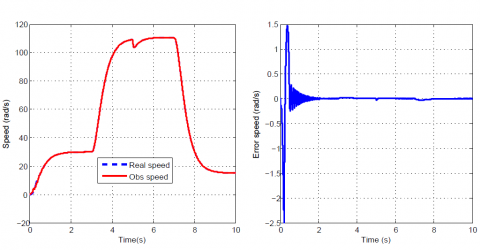
Figure 3. (a) Actual and estimated speeds of IPMSM; (b) Error speed
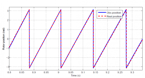
Figure 4. Actual and estimated rotor position of IPMSM
All simulation results are shown in figures from Figure 3 to Figure 9. They are given to show the efficiency of the sliding mode based sensorless speed control of IPMSM in a wide speed range.
Figure 5. Active flux estimated
Figure 6. $\hat{i}_{d} \hat{i}_{q}$estimated currents
Figure 7. (a) Actual and estimated speeds at +50R% (b) Error speed at +50R%
Figure 8. Actual and estimated rotor position of IPMSM at +50R%
Figure 9. $\hat{i}_{d} \hat{i}_{q}$ estimated currents at +50R%
The motor starts from 0 rad/s to 30 rad/s. After that acceleration from 30 rad/s to 150 rad/s over the rated speed is realized at t=3s. A load of 5 Nm is applied to the motor at t=5s.This causes instantaneous reduction of the speed. Finally deceleration from 150 rad/s to 5 rad/s is simulated. This figure demonstrates the effectiveness of the observer estimation in the wide speed range.
The rotor speed estimation shown in Figure 3 (a) and estimated position shown in Figure 4 tracks the actual rotor speed and the real position respectively
it can be noticed that the proposed SMO works very well in the very low speed region. We note also that the expected speed error shown in Figure 3(b) becomes zero after few seconds
Figure 5 presents the corresponding active flux curve. It can be noted that it is always constant in steady state regime and equal to that induced by the permanent magnet because the d-axis current is maintained to zero.
Figure 6 shows $\hat{\imath}_{d}$ and $\hat{\imath}_{q}$ estimated currents component. It appears that the stator current was well controlled showing the performance of current regulator in the proposed sensorless control structure.
The stator resistance variation test is introduced to verify the robustness of the proposed feedback control. It can be seen from Figure 7 to 9, that SMO is still able to obtain good estimation of position and rotor speed of IPMSM even if +50%±50% resistance variation occurred.
We can conclude from previous simulations results that the sliding mode observer provides good estimation of position and rotor speed for wide speed range particularly at low speed with and without load.
To overcome speed sensors issues such as cost and vulnerability, a Sliding Mode Observer for Sensorless Speed Control of IPMSM Based on Active Flux Concept has been proposed. Some advantages can be cited for this method. Among these advantages, the active flux concept was used to reduce the IPMSM dynamical model complexity in the (α,β) reference frame and to facilitate SM observer design. From this study, one can conclude the effectiveness of sliding mode observer and a good performance at low speed range when motor parameter variations occurred. The simulation results confirm the effectiveness of this approach.
|
uα, uβ |
Voltage on the fixed coordinate |
|
iα, iβ |
Current on the fixed coordinate |
|
wr |
Mechanical rotor speed |
|
q |
Rotor position |
|
R |
Stator resistance |
|
p |
Differential operator |
|
KE |
EMF constant |
|
M |
Mutual inductance |
|
Ld |
d-axis inductance |
|
Lq |
q-axis inductances |
|
Te |
Electromagnetic torque |
|
P |
Number of pole pairs |
|
jf |
Rotor flux |
|
jd |
Active flux |
|
Tl |
Load torque |
|
J |
Moment of inertia |
|
f |
Friction coefficient |
|
IPMSM |
Interior permanent magnet synchronous motor |
|
SPMSM |
Surface permanent magnet synchronous motor |
|
SMO |
Sliding mode observer |
|
EMF |
Extended back-electromotive force |
[1] Bechkaoui, A., Ameur, A., Bouras, S., Ouamrane, K. (2015). Diagnosis of turn short circuit fault in PMSM sliding-mode control based on adaptive fuzzy logic-2 speed controller. AMSE J. Ser. Adv. C, 70(1): 29-45.
[2] Morimoto, S., Sanada, M., Takeda, Y. (1994). Wide-speed operation of interior permanent magnet synchronous motors with high-performance current regulator. IEEE Transactions on Industry Applications, 30(4): 920-926. https://doi.org/10.1109/28.297908
[3] Rahman, M.A. (2005). Advances in interior permanent magnet (IPM) motor drives. In 2005 IEEE Power Engineering Society Inaugural Conference and Exposition in Africa, pp. 372-377. https://doi.org/10.1109/PESAFR.2005.1611848
[4] Chen, Z., Tomita, M., Ichikawa, S., Doki, S., Okuma, S. (2000). Sensorless control of interior permanent magnet synchronous motor by estimation of an extended electromotive force. In Conference Record of the 2000 IEEE Industry Applications Conference. Thirty-Fifth IAS Annual Meeting and World Conference on Industrial Applications of Electrical Energy (Cat. No. 00CH37129), 3: 1814-1819. https://doi.org/10.1109/IAS.2000.882126
[5] Morimoto, S., Sanada, M., Takeda, Y. (2006). Mechanical sensorless drives of IPMSM with online parameter identification. IEEE Transactions on Industry Applications, 42(5): 1241-1248. https://doi.org/10.1109/TIA.2006.880840
[6] Hasegawa, M., Yoshioka, S., Matsui, K. (2009). Position sensorless control of interior permanent magnet synchronous motors using unknown input observer for high-speed drives. IEEE Transactions on Industry Applications, 45(3): 938-946. https://doi.org/10.1109/TIA.2009.2018968
[7] Jang, J.H., Ha, J.I., Ohto, M., Ide, K., Sul, S.K. (2004). Analysis of permanent-magnet machine for sensorless control based on high-frequency signal injection. IEEE Transactions on Industry Applications, 40(6): 1595-1604. https://doi.org/10.1109/TIA.2004.836222
[8] Zhu, H., Xiao, X., Li, Y. (2009). A simplified high frequency injection method for PMSM sensorless control. In 2009 IEEE 6th International Power Electronics and Motion Control Conference, pp. 401-405. https://doi.org/10.1109/IPEMC.2009.5157420
[9] Medjmadj, S., Diallo, D., Mostefai, M., Delpha, C., Arias, A. (2014). PMSM drive position estimation: Contribution to the high-frequency injection voltage selection issue. IEEE Transactions on energy conversion, 30(1): 349-358. https://doi.org/10.1109/TEC.2014.2354075
[10] Cho, Y. (2016). Improved sensorless control of interior permanent magnet sensorless motors using an active damping control strategy. Energies, 9(3): 135. https://doi.org/10.3390/en9030135
[11] Peixoto, Z.M.A., Sa, F.M.F., Seixas, P.F., Menezes, B.R., Cortizo, P.C. (1995). Design of sliding observer for back electromotive force position and speed estimation of interior magnet motors. In EPE, 95: 833-838.
[12] Shi, J.L., Liu, T.H., Chang, Y.C. (2007). Position control of an interior permanent-magnet synchronous motor without using a shaft position sensor. IEEE Transactions on Industrial Electronics, 54(4): 1989-2000. https://doi.org/10.1109/TIE.2007.895137
[13] Luiz, A.D.S., Harke, M.C., Lorenz, R.D. (2006). Dynamic properties of back-emf based sensorless drives. In Conference Record of the 2006 IEEE Industry Applications Conference Forty-First IAS Annual Meeting, 4: 2026-2033. https://doi.org/10.1109/IAS.2006.256814
[14] Nahid-Mobarakeh, B., Meibody-Tabar, F., Sargos, F.M. (2007). Back EMF estimation-based sensorless control of PMSM: Robustness with respect to measurement errors and inverter irregularities. IEEE Transactions on Industry Applications, 43(2): 485-494. https://doi.org/10.1109/TIA.2006.889826
[15] Inoue, Y., Yamada, K., Morimoto, S., Sanada, M. (2009). Effectiveness of voltage error compensation and parameter identification for model-based sensorless control of IPMSM. IEEE Transactions on Industry applications, 45(1): 213-221. https://doi.org/10.1109/TIA.2008.2009617
[16] Chen, Z., Tomita, M., Doki, S., Okuma, S. (2003). An extended electromotive force model for sensorless control of interior permanent-magnet synchronous motors. IEEE transactions on Industrial Electronics, 50(2): 288-295. https://doi.org/10.1109/TIE.2003.809391
[17] Boldea, I., Paicu, M.C., Andreescu, G.D. (2008). Active flux concept for motion-sensorless unified AC drives. IEEE Transactions on Power Electronics, 23(5): 2612-2618. https://doi.org/10.1109/TPEL.2008.2002394
[18] Koonlaboon, S., Sangwongwanich, S. (2005). Sensorless control of interior permanent-magnet synchronous motors based on a fictitious permanent-magnet flux model. In Fourtieth IAS Annual Meeting. Conference Record of the 2005 Industry Applications Conference, 2005, 1: 311-318. https://doi.org/10.1109/IAS.2005.1518326
[19] Koteich, M., Duc, G., Maloum, A., Sandou, G. (2016). A unified model for low-cost high-performance ac drives: the equivalent flux concept. In 2016 Third International Conference on Electrical, Electronics, Computer Engineering and their Applications (EECEA), 71-76. https://doi.org/10.1109/EECEA.2016.7470768
[20] Qiao, Z., Shi, T., Wang, Y., Yan, Y., Xia, C., He, X. (2012). New sliding-mode observer for position sensorless control of permanent-magnet synchronous motor. IEEE Transactions on Industrial Electronics, 60(2): 710-719. https://doi.org/10.1109/TIE.2012.2206359
[21] Belhamdi, S., Goléa, A. (2011). Sliding mode control of asynchronous machine presenting defective rotor bars. AMSE Journals, Series Advances C, 66(1/2): 39-49.
[22] Rahali, H., Zeghlache, S., Benalia, L., Layadi, N. (2018). Sliding mode control based on backstepping approach for a double star induction motor (DSIM). AMSE Journals, Advances in Modelling and Analysis C, 73(4): 150-157.
[23] Feng, Y., Zheng, J., Yu, X., Truong, N.V. (2009). Hybrid terminal sliding-mode observer design method for a permanent-magnet synchronous motor control system. IEEE Transactions on Industrial Electronics, 56(9): 3424-3431. https://doi.org/10.1109/TIE.2009.2025290
[24] Yuan, Q., Yang, Z., Lin, F., Sun, H. (2013). Sensorless Control of Permanent Magnet Synchronous Motor with Stator Flux Estimation. JCP, 8(1): 108.
[25] Hermann, R., Krener, A. (1977). Nonlinear controllability and observability. IEEE Transactions on automatic control, 22(5): 728-740. https://doi.org/10.1109/TAC.1977.1101601
[26] Boukhobza, T., Barbot, J.P. (1998). Step by step sliding mode observer for implicit triangular observer form. IFAC Proceedings Volumes, 31(17): 231-236. https://doi.org/10.1016/S1474-6670(17)40340-5
[27] Ezzat, M. (2011). Sensorless nonlinear control of a permanent magnet synchronous motor (Doctoral dissertation, Phd thesis, Institut de Recherche en Communications et en Cybernétique de Nantes, Sept 2011).
[28] Sosse Alaoui, M.C. (2009). Sliding modes control and observer for a pumping system and a manipulator arm. Doctoral thesis, University of Sidi Mohammed Ben Abdellah. Fès, 74-76.