Ranjith Kumar Gatla | M Ramesh | Kota Prasada Rao | P Shashavali | Durga Prasad Garapati | P Chandra Babu | Devineni Gireesh Kumar*
© 2023 IIETA. This article is published by IIETA and is licensed under the CC BY 4.0 license (http://creativecommons.org/licenses/by/4.0/).
OPEN ACCESS
The number of cycles to the end of life for high-power IGBT modules is expressed as a function of the stress parameters in the model. Most of the time, these models are generated on the basis of experimental data from accelerated power-cycling experiments that are done at preset temperatures and stress levels. This paper proposed a systematic Reliability evaluation process for large-scale commercial and utility-level PV power systems. The major contribution of this work is the quantification of the impact of junction temperature on the failure rates of critical components such as PV Inverters and capacitors. Usually, the reliability assessment of the power electronic switch such as IGBT and inverter focused on component level, whereas much fewer cases discussed the Reliability evaluation for the entire PV system. In light of the above concerns, this article discussed the effect of junction temperature on the lifetime of IGBT modules, and the relevant lifetime factor is modelled. This study enables us to include the junction temperature effect on the lifetime model of IGBT modules under the given mission profiles of the converter.
junction temperature, IGBT, lifetime assessment, thermal analysis, PV systems
In terms of their use in high-power converters, insulated gate bipolar transistors (IGBTs) are widely regarded as the most common type of device. IGBTs are very sensitive devices, and their failure can cause severe problems [1-2]. Power converter reliability is determined by a thorough knowledge of the failure processes of inductively coupled bipolar transistor (IGBT) modules, as well as the availability of validated lifespan models. The reliability of IGBT power modules has been assessed using failure data collected in the field [3-4] as well as accelerated power cycling tests (PCTs) [5]. However, since it takes such extended periods of observation, the first technique is not particularly practical. The accelerated PCT method is, therefore, widely used for analyzing the long-term reliability of high-power IGBT modules, as well as for modelling their predicted lifespan [6], among other things.
For developing lifetime models for various kinds of IGBT modules, the data collected from various devices under test is analyzed. The models are based on the various operational and structural parameters of the device. They show the number of stress cycles that the device experiences due to these factors. Some of these include the junction temperature swing, the cooling current, and the heating current. It has been created and confirmed in the literature that two noteworthy empirical lifespan models, often referred to as the LESIT [7] and the CIPS08 [8], are used. Empirical lifespan models are unable to discriminate between failure mechanisms, and a post-mortem investigation is required to determine the most likely cause of death. When an IGBT reaches the end-of-life (EOL), three separate failure modes have been identified: bond-wire lift-offs, die solder delamination, and substrate solder delamination [9]. Even though these mechanisms are being created concurrently, the major cause of failure is dependent on the stressful circumstances that are present.
PV power systems are a major source of renewable energy. They have zero greenhouse gas emissions and are able to produce electricity without using fossil fuels. The total installed capacity of PV power systems has increased from 80 GW in 2016 to over 210 GW in 2022. The average annual growth rate of the PV power system market has been around 21.66% from 2016 to 2022. It is expected to increase to around 50% in 2025 [9]. The continuous availability of reliable PV power systems will greatly increase renewable energy output and help reduce greenhouse gas emissions [10].
Unlike other electrical systems, such as batteries, PV power systems can fail due to various factors, such as mechanical failure or accidental events. The reliability of PV power systems has been a major concern for the customers and the utility companies. A PV power system is made up of various components, such as solar cells etc [11]. These components have varying life cycle reliability depending on the ambient conditions and load. One of the most vulnerable components of a PV power system is the power electronic device known as an inverter. This component can operate at high temperatures andexpose its components to higher energy losses.
High energy losses can lead to the degradation of the core temperature of the switching devices, which can affect the system's overall reliability. The reliability of an inverter is dependent on the ambient temperature, its solar light intensity, and its input power levels [12]. This paper aims to analyze the various factors that affect the reliability of an inverter.
Figure 1. Renewable annual net capacity additions by Technology 2016 – 2022 [12]
The complexity of PV power systems makes it difficult to analyze their reliability performance. Most of the current literature on PV power system reliability focuses on the assessment of power electronic components. Less attention is given to the evaluation of the entire system. In [13], various contributions to the field of PV reliability have been presented. The failure rates and probabilities of electronic components in a PV system are treated as constants. The various parameters of the PV system's reliability are not always the same as they are in the case of other systems. For instance, the cost of a PV inverter failure is typically around 59% of the system's total cost. The lifetime prediction of a PV system's inverter is a crucial factor that influences the design and operational costs of a system.
The lifetime of a PV system's inverter can affect the thermal loading of the device. This is because the stress that the semiconductor material can endure during operation affects its properties. The stress that a semiconductor device can endure during operation is indirectly related to its temperature. By taking into account the various layers of a semiconductor, the lifetime of the device can be determined [14]. The constant temperature and the irradiance of the solar radiation can cause non-uniform thermal stress over a year. This is because the temperature variation can affect different regions and seasons.
The temperature also affects the lifetime prediction of a PV system's inverter. If the temperature exceeds the rated values, it will cause more losses. This is why the power conversion system's thermal management must be performed properly. In [15] presented two typologies for the reliability of power electronics components. The authors of this paper used an approximate method to perform a better comparison between the parts count method and the parts stress method. A direct correlation is performed between the temperature and the failure rate of various power electronic components [16]. They used the power loss in switches and diodes as an example. The exact method performed by the authors of this paper is different from the other methods. The advantage of using the exact method is that it takes into account the various conditions of the system's inverter. The paper aims to analyze the trade-off between the high reliability of power semiconductor devices and the low cost of them. A study conducted before switching to a device with a larger current rating revealed that a higher current rating can increase the operating hours of the device. The design of an IGBT should also be considered when it comes to optimizing the system's operating hours. Doing so will help determine the optimal solution for the system.
1.1 Problem statement
With the advancement of chip, packaging and manufacturing technologies, IGBT suppliers are continuously improving their component Reliability performance. Therefore, in most applications, power electronics designers can easily find available IGBTs that can achieve the required lifetime specifications. The practical problem for them is how to selectthe proper IGBTs to fulfil the Reliability target while minimizing cost. This is especially true in the PV industry, having a very stringent cost constraint to reduce the cost of electric power generation. However, due to the following challenges, the Reliability analyses of the IGBTs designed in PV Inverters are usually not well treated, resulting in either a lack of robustness or over-design with unnecessary cost increase. Further on, this research intends to cover two principal aspects when predicting the lifetime of switching devices.
1.2 Methodology
Various procedures have been introduced in the past few decades to estimate the reliability of a PV system. The first one was published in 1956 by the Rome Air Development Centre. This standard describes the failure rate for electronic devices. After the publication of MIL-HDBK-217, it became the most popular handbook in this field. Various organisations and firms improved their Reliability after reading this handbook. Reliability can be predicted using a part stress method. This method involves analysing the electrical components and circuits. The part count method is generally less data-intensive. It involves collecting information about the various components and their quality conditions. The accuracy of part stress methods is usually higher than that of part count methods. The main difference between the two is that part stress methods take into account the failure rate of the system.
An inverter is an electrical device that converts power from one source to another. It can be used in various appliances. DC is commonly used in various electrical equipment, such as solar power systems. Most of these are powered by direct current, which is produced by the batteries, fuel cells, and power sources. An inverter can convert this current into AC power. AC power can be used by residential and industrial consumers and those using the public utility grid. In alternating power systems, the batteries can store DC power. Aside from powering some electrical equipment, such as home appliances, AC power can also be used for other functions. An inverter can be used forvarious applications, such as solar power. There are various types of these devices available in the market. DC power sources are used to provide an AC voltage to electronic equipment and electrical equipment, such as home appliances.
2.1 Working of inverter
An inverter uses a DC source to convert the current into AC power. In most cases, this technology does not generate any power. However, in some situations, such as when the DC voltage is low, an appliance cannot use the low DC voltage. Due to this, an inverter can be used in solar power systems. In this case, the power circuit of the device is composed of four bidirectional IGBTs. Figure 2 shows the power circuit diagram of the device.
Figure 2. H-Bridge Inverter Topology
Mode 1: Current conduction when S4 and S1 are ON
The four IGBTs power the device's power circuit. When the S1 and S4 are activated, the output of the device is converted to DC. This ensures that the load is always applied evenly. The current starts from the positive supply, S1, and ends at the negative supply, S2. The conduction path of the device's first cycle is shown in Figure 3.
Figure 3. Current conduction when S4 and S1 are ON
Mode 2: Current conduction when S2 and S3 are ON
The device's next cycle begins after the trigger pulse of the IGBT S2 is sent to the gate. During this period, the input voltage is applied in the negative direction. The current flows from the positive supply to the negative supply and then to the negative supply. The current path of the device's next cycle is shown in Figure 4.
Figure 4. Current conduction when S2 and S3 are ON
The two cycles continue to produce a positive and a negative voltage. When the current direction changes, the load gets adjusted. As the current changes, the voltage at the load is converted to an AC voltage. This is done to convert the DC voltage into the AC.
One of the most critical factors that a power electronics system should consider is the proper thermal design. This ensures that its components will have a long life. In addition to the thermal design, a power semiconductor's thermal equivalent model is also used for the design. This chapter presents an example of an IGBT module. After a review of the model, a final step is performed to implement the design.
3.1 Power loss calculation model
The total power losses of an IGBT module are calculated by taking into account the switching and conduction losses. The power loss modelling process is carried out using the look-up tables provided by the manufacturers of the printed circuit materials. It is mainly done for the sake of simplicity and the project's requirements. The power losses of various semiconductor components can also be calculated:
a) Switching losses ( $\left.\mathrm{P}_{\mathrm{SW}}\right)$
b) Conduction losses ( $\left.\mathrm{P}_{\mathrm{COND}}\right)$
Therefore: $\mathrm{P}_{\text {LOSS }}=\mathrm{P}_{\text {COND }}+\mathrm{P}_{\mathrm{SW}}$
3.2 Transient thermal impedance $\mathrm{Z}_{\mathrm{th}(\mathrm{J}-\mathrm{C})}(\mathrm{T})$
In terms of the transient thermal behavior of a device, such as an IGBT module, the $Z_{\text {th }}$ is the number of times its voltage is changed. The equation also determines the impedance of a chip or a device.
$Z_{\text {th }}$ $(j-c)(t)=\frac{\operatorname{Tj}(t)-T c(t)}{\text { Ploss }}$ (1)
where,
$\mathrm{T}_{\mathrm{j}(\mathrm{t})}$ and $\mathrm{T}_{\mathrm{c}(\mathrm{t})}$ are defined as Junction and Case Temperature Respectively.
$P_{\text {loss }}$ is the power loss of an IGBT or a diode chip.
3.2.1 Cauer Model
The Cauer Model is used for the thermal design of an IGBT module. It allows engineers to understand the thermal behavior of the device. As shown in Figure 5. The goal of this model is to provide a physical image of the internal thermal behavior of an IGBT module. It is also necessary to acquire the various properties of the various layers inside the device. Nevertheless, the use of the Cauer Model in designing power electronics systems is not practical for most IGBT users. It can be hard for them to visualize the model's details and make informed decisions.
Figure 5. Cauer Model
3.2.2 Foster Model
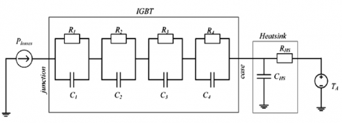
The Foster Model is a more practical alternative to the Cauer Model. It consists of a series of connected RC elements, as shown in Figure 6. Each element has its parallel circuit. Unlike the Cauer Model, the Foster Model does not have physical significance. It is useful in developing power electronics systems since it does not require detailed information about the various layers in an IGBT device. The model's thermal impedance is derived from the circuit shown in Figure 6. The $\mathrm{Z}_{\mathrm{th}}$ value of the model is expressed as follows.
$\operatorname{Zth}(\mathrm{j}-\mathrm{c})(\mathrm{t})=\sum_{i=1}^n \operatorname{Ri}\left(1-e^{-\frac{t}{T i}}\right)$ (2)
where, $\tau_i=R_i \times C_i$. This model is realized by tuning the model's characteristics to the transient thermal impedance described in a data sheet.
Figure 6. Foster Form
Since the goal of every manufacturer is to maximize the efficiency of their products, they have always been striving for the highest output quality. In addition, having a longer lifespan can help minimize energy consumption and improve the reliability of their power converters. The reliability of a system is a statistical measure that shows the likelihood of failure at a given time. It can be divided into smaller parts and is evaluated through various factors. Researchers use various statistical measures to determine the reliability of a system. Some of these include the failure rate, the mean time to failure, and the availability of repairs.
4.1 Failure
A failure occurs when the system stops performing a task for any reason. This variable is a random one, and it can be long or short. There are two types of failure: gradual and sudden. The former is referred to as degradation failure, while the latter is called cataleptic failure.
4.2 Failure rate
The failure rate function is a vital part of assessing the system's reliability. It can help predict the probability of failure over some time. It can be calculated by taking the time unit that has elapsed since the last failure.
Failure rate $\mathrm{f}(\mathrm{t}, \lambda)=\lambda \mathrm{e}^{-\lambda \mathrm{t}}$ (3)
4.3 Mean Time To Failure (MTTF)
The mean time to failure is the average before a device or component gets its first failure. This type of failure occurs when the device's functions are no longer possible. The maximum time to failure, or MTTF, is usually calculated in hours or thousand hours. When the maximum MTTF of a device is reported, it means that the first failure that can cause the device to malfunction is expected to happen after this period.
$\mathrm{MTTF}=1 / \lambda$ (4)
4.4 Mean Time To Repair (MTTR)
The average time it takes to repair a failed device is known as the MTTR. This value is computed by taking into account the condition of the system, and its gamma distribution can be given as
$\operatorname{MTTR}=\beta / \mu$ (5)
4.5 Mean Time Between Failures (MTBF)
The average time that a system has gone without experiencing a failure is referred to as the MTBF. In some cases, the definitions of this measure do not describe the reliability of the system. In other cases, it can be useful to measure the likelihood of a system experiencing an emergency failure.
$\mathrm{MTBF}=\mathrm{MTTF}+\mathrm{MTTR}$ (6)
4.6 Reliability methodology
Various procedures have been introduced in the past decades for estimating the reliability of various products. The first such standard was established in 1956 by the RADC in the US. It was entitled TR-1100. This was a reference for estimating the failure rate of electronic and computer components. The following year, the standard was updated and became a handbook for estimating the reliability of various products. After that, various companies and organizations started developing their software and handbooks for this field. This standard has been proven to be more reliable than other ones due to its various factors. It covers all aspects of reliability. This handbook uses two methods to estimate the reliability of various components. Parts count, and parts stress are used to calculate the total reliability of a system. The parts stress method is able to predict the reliability of an electrical system due to the stress that the components and circuits under stress undergo. The parts count method is generally less demanding than the parts stress method. It provides information about the number of components and their quality, which helps yield more accurate results.
4.6.1 Parts count method
One of the most common approaches used in assessing the reliability of a system is parts count. This method takes into account the various components of a system and then uses a simple statistical method to conclude. This method is usually used when there is no detailed information about the system. It takes into account the operating conditions of the system and then comes up with a conclusion. It is not always possible to determine the reliability of a system based on its operating conditions. For instance, if the device is not working properly, the parts count method might not provide a conclusive conclusion. The parts count method is approximate since it only takes into account the number of components. The parts count method is usually performed based on quantitative analyses.
$\lambda_{\text {system }}=\sum_{i=1}^N \lambda_{\text {ref(i) }} * \mathrm{k}$ (7)
where,
$\mathrm{K}$ is the number of elements with the reference failure rate of ref (i).
$\mathrm{N}$ is the number of parts.
4.6.2 Parts stress method
The parts stress method is a set of procedures designed to calculate the stress levels of various components. Unlike the parts count method, this method involves knowing the specific operating conditions and stress levels of the parts. The parts stress method is used to evaluate the reliability of a system. It involves determining the various stresses that each component experiences during its operation. The conditions that are shown in the failure rate equations can be shown by the various pi factors in the method. However, the number of parameters used in this method can lead to complexity in calculating the failure rates. The total failure rate of a system can be calculated by summing the various failure rates. This method is similar to the parts count method.
The $\lambda$ is calculated as follows
$\lambda_{\mathrm{b}}=\mathrm{A}^* \exp \left[\frac{N_T}{273+T+(\Delta T) s}\right] *\left[\frac{273+T+(\Delta T) s}{N_T}\right]^p$ (8)
where,
A is the scaling factor of the failure rate.
$\mathrm{N}_{\mathrm{T}}, \mathrm{T}_{\mathrm{M}}$, and $\mathrm{P}$ are the shape parameters.
$\mathrm{T}$ is the Temperature.
$\Delta \mathrm{T}$ is the difference between the maximum allowable temperature with no junction current and full-rated junction current or power.
$\mathrm{S}$ is the stress ratio that the ratio of actual stress to rated stress can be calculated.
A combined approach to predict the reliability of a system involves taking into account the various parts of the system. This model ensures that the system's overall reliability is determined as
$\lambda \mathrm{p}=\lambda_{\mathrm{O}} \pi_{\mathrm{O}}+\lambda_{\mathrm{C}} \pi_{\mathrm{C}}$ (9)
where,
$\lambda \mathrm{p}$ is the predicted failure rate.
$\lambda_0$ is the failure rate from operational stresses.
$\lambda_{\mathrm{C}}$ is the failure rate caused by temperature cycling stresses.
$\pi_{\mathrm{C}}$ is the cycling factor.
The reliability of various electronic components has been studied. These include switches, capacitors, and inductors. The various relationships and equations that have been presented have shown how these components can fail. In this paper, we discuss the failure rate of various electronic components that are commonly used in power electronic circuits.
$\lambda_{\mathrm{p}}($ Capacitor $)=\lambda_{\mathrm{b}} \pi_{\mathrm{CV}} \pi_{\mathrm{Q}} \pi_{\mathrm{E}}$ (10)
$\lambda_{\mathrm{p}}($ Inductor $)=\lambda_{\mathrm{b}} \pi_{\mathrm{C}} \pi_{\mathrm{Q}} \pi_{\mathrm{E}}$ (11)
$\lambda_{\mathrm{p}}($ Switch $)=\lambda_{\mathrm{b}} \pi_{\mathrm{T}} \pi_{\mathrm{A}} \pi_{\mathrm{Q}} \pi_{\mathrm{E}}$ (12)
$\lambda_{\mathrm{p}}($ Diode $)=\lambda_{\mathrm{b}} \pi_{\mathrm{T}} \pi_{\mathrm{c}} \pi_{\mathrm{s}} \pi_{\mathrm{Q}} \pi_{\mathrm{E}}$ (13)
where,
$\lambda_{\mathrm{b}}$ is the base failure rate, which is 0.012 and 0.064 for switch and diode, respectively.
$\lambda_{\mathrm{b}}($ inductor $)=0.00035 * \exp \left[\frac{T_{h s}+273}{326}\right]^{15.6}$ (14)
$\lambda_{\mathrm{b}}($ Capacitor $)=0.00254\left[\left(\frac{s}{0.5}\right)^3+1\right] \exp \left[5.09\left(\frac{T A+273}{378}\right)^5\right]$ (15)
|
$\mathbf{T}_{\mathrm{C}}$ |
$\pi_A$ |
$\pi_Q$ |
$\pi_E$ |
$\lambda_b$ |
|
25 |
10 |
5.5 |
1 |
0.012 |
where,
$\mathrm{T}_{\mathrm{HS}}$ is the heat sink temperature.
$\mathrm{S}$ is the ratio of operating voltage to nominal voltage.
In Equation (14), $\mathrm{T}_{\mathrm{HS}}$ is calculated as follows:
$\mathrm{T}_{\mathrm{HS}}=\mathrm{T}_{\mathrm{A}}+1.1+\Delta \mathrm{T}$ (16)
where,
$\mathrm{T}_{\mathrm{A}}$ is the device's ambient operating temperature (in degrees Celsius).
$\Delta \mathrm{T}$ is the average temperature rise above ambient.
In switch and diode failure rates (equation (12), equation (13)), $\pi_{\mathrm{T}}$ is the Temperature factor and can be calculated as shown below:
$\pi_{\mathrm{T}}(\mathrm{S})=\exp \left[-1925\left(\frac{1}{T j+273}-\frac{1}{298}\right)\right]$ (17)
$\pi_{\mathrm{T}}(\mathrm{D})=\exp \left[-1925\left(\frac{1}{T j+273}-\frac{1}{293}\right)\right]$ (18)
$\mathrm{T}_{\mathrm{j}}$ is the junction temperature and must be obtained by the following equation:
$\mathrm{T}_{\mathrm{j}}=\mathrm{T}_{\mathrm{C}}+\theta_{\mathrm{JC}} * \mathrm{P}_{\text {loss }}$ (19)
where,
$\mathrm{T}_{\mathrm{C}}$ is the heat sink temperature.
$\theta_{\mathrm{Jc}}$ is the thermal resistance of the diode or switch ( 0.25 for the switch and 1.6 for the diode).
$P_{\text {loss }}$ is the power loss of a switch or diode.
$\pi_S$ is the stress factor and is calculated as follows:
$\pi_{\mathrm{S}}=v_s^{2.43}$ (20)
where,
$\mathrm{V}_{\mathrm{S}}$ is the ratio of operating voltage to nominal voltage.
In equation (10), $\pi_{\mathrm{CV}}$ is the capacitor factor which can be obtained by:
$\pi \mathrm{CV}=0.34 * c^{0.12}$ (21)
where, $\mathrm{C}$ is the capacitance value (in microfarad).
In some cases, the values of quality factor and environment factor $Q$ have been ignored. To improve the accuracy of the calculations, the values of these two factors can be considered as environment factor $\mathrm{E}$ for all components. For instance, the values of 10, 5.5, and 20 for inductors, semiconductors, and capacitors, respectively, are considered as environment factor $E$ for all electronic components.
The temperature factor is a crucial factor that affects the reliability of power electronic devices. It is used in the calculation of power losses for various semiconductor components, such as IGBTs and diodes. The failure rate of these components depends on the method used for calculating power losses.
The Reliability Evaluation of the Photo Voltaic Inverter and its comparison are simulated in PLECS Blockset. The Reliability evaluation of the Photo Voltaic Inverter is designed and simulated in PLECS. Table 1 shows the specifications of the Photo Voltaic Inverter.
Table 1. Specifications of the Photo Voltaic Inverter
|
S. No |
Parameter |
Range |
|
1. |
PV Cell Voltage |
400 V (avg) |
|
2. |
PV Cell Current |
7.5 A (avg) |
|
3. |
PV Cell Power |
3000 W (avg) |
|
4. |
Inverter Voltage |
230 V (rms) |
|
5. |
Inverter Current |
13 A (rms) |
|
6. |
Inverter Power |
3000 W (rms) |
Figure 7. Thermal model of a PV Bridge Inverter
Figure 7 shows the Thermal modeling of a PV Bridge Inverter. Figure 8 shows the Output voltage, current, and power of a PV Inverter with an output DC voltage, DC, and DC power of 400 Volts, 7.5Amps and 3000 Watts, respectively. Figure 9 shows the Output voltage, current, and power of a Grid with an output $\mathrm{AC}$ voltage, $\mathrm{AC}$, and $\mathrm{AC}$ power of 230 Volts, 13 Amps, and 3000 Watts, respectively.
Figure 8. Output voltage, current, and power of a PV cell
Figure 9. Output voltage, current, power of a Grid
5.1 Practical calculations for reliability
In order to calculate the lifetime of an IGBT, we should find out the junction temperature of the IGBT module. We can calculate the junction temperature using PLECS; by substituting the junction temperature in the exact method, we can get the Reliability of that IGBT. For calculating the Reliability, we assumed different inverters listed below.
$\lambda_{\mathrm{p}}($ Switch $)=\lambda_{\mathrm{b}} * \pi_{\mathrm{T}} * \pi_{\mathrm{A}} * \pi_{\mathrm{Q}} * \pi_{\mathrm{E}}$
where,
$\lambda_{\mathrm{p}}$ = Predicted failure rate
$\lambda_{\mathrm{b}}$ = Base failure rate
$\pi_{\mathrm{T}}$ = Temperature factor
$\pi_{\mathrm{Q}}$ = Environmental Factor
$\pi_{\mathrm{E}}$ = operational stresses
$\pi_{\mathrm{T}}(\mathrm{S})=\exp \left[-1925\left(\frac{1}{T j+273}-\frac{1}{298}\right)\right]$
where,
$\mathrm{T}_{\mathrm{J}} =$ Junction Temperature
Mean Time To Failure $=1 / \lambda$
where,
$\lambda=$ Predicted failure rate
Case (i): Analysis for 45A IGBT
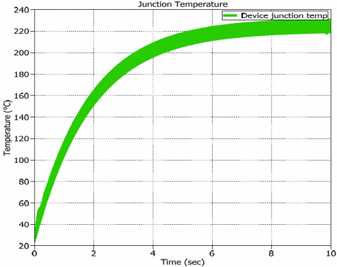
Figure 10. Junction temperature for 45A IGBT
Junction temperature for 400V & 45A IGBT module is 232.66°C. From equation 17, Reliability is evaluated as follows.
$\begin{aligned} \pi_{\mathrm{T}}(\mathrm{S}) & =\exp \left[-1925\left(\frac{1}{T j+273}-\frac{1}{298}\right)\right] \\ & =\exp \left[-1925\left(\frac{1}{232.66+273}-\frac{1}{298}\right)\right] \\ & =14.1940\end{aligned}$
$\begin{aligned} \lambda_{\mathrm{p}}(\text { Switch }) & =\lambda_{\mathrm{b}} * \pi_{\mathrm{T}} * \pi_{\mathrm{A}} * \pi_{\mathrm{Q}} * \pi_{\mathrm{E}} \\ & =0.012 * 14.1940 * 10 * 5.5 * 6 \\ & =56.208\end{aligned}$
$\begin{aligned} \operatorname{MTTF} \text { for IGBT }(\mathrm{t}) & =1 / \lambda \\ & =1 / 56.208 \\ & =17790.87 \text { Hours }\end{aligned}$
$\begin{aligned} \text { MTTF for inverter } & =4 * \text { MTTF for IGBT } \\ & =4 * 17790.87 \\ & =71163.48 \text { Hours }\end{aligned}$
Case (ii): Analysis for 60A IGBT
Figure 11. Junction temperature for 60A IGBT
Junction temperature for 400V & 60A IGBT module is 227.45°C. From equation 17, Reliability is evaluated as follows.
$\begin{aligned} \pi_{\mathrm{T}}(\mathrm{S}) & =\exp \left[-1925\left(\frac{1}{T j+273}-\frac{1}{298}\right)\right] \\ & =\exp \left[-1925\left(\frac{1}{227.45+273}-\frac{1}{298}\right)\right] \\ & =13.6426\end{aligned}$
$\begin{aligned} \lambda_{\mathrm{p}}(\text { Switch }) & =\lambda_{\mathrm{b}} * \pi_{\mathrm{T}} * \pi_{\mathrm{A}} * \pi_{\mathrm{Q}} * \pi_{\mathrm{E}} \\ & =0.012 * 13.6426 * 10 * 5.5 * 6 \\ & =54.0429\end{aligned}$
$\begin{aligned} \text { MTTF for IGBT }(\mathrm{t}) & =1 / \lambda \\ & =1 / 54.0429 \\ & =18509.98 \text { Hours }\end{aligned}$
$\begin{aligned} \text { MTTF for inverter } & =4 * \text { MTTF for IGBT } \\ & =4 * 18509.98 \\ & =74039.92 \text { Hours }\end{aligned}$
Case (iii): Analysis for 90A IGBT
Figure 12. Junction temperature for 90A IGBT
The junction temperature for the 400V & 90A IGBT module is 227.45°C. From equation 17, Reliability is evaluated as follows.
$\begin{aligned} \pi_{\mathrm{T}}(\mathrm{S}) & =\exp \left[-1925\left(\frac{1}{T j+273}-\frac{1}{298}\right)\right] \\ & =\exp \left[-1925\left(\frac{1}{201.147+273}-\frac{1}{298}\right)\right] \\ & =11.0210\end{aligned}$
$\begin{aligned} \lambda_{\mathrm{p}}(\text { Switch }) & =\lambda_{\mathrm{b}} * \pi_{\mathrm{T}} * \pi_{\mathrm{A}} * \pi_{\mathrm{Q}} * \pi_{\mathrm{E}} \\ & =0.012 * 11.0210 * 10 * 5.5 * 6 \\ & =43.643\end{aligned}$
$\begin{aligned} \operatorname{MTTF} \text { for IGBT }(\mathrm{t}) & =1 / \lambda \\ & =1 / 43.643 \\ & =22912.94 \text { Hours }\end{aligned}$
$\begin{aligned} \text { MTTF for inverter } & =4 * \text { MTTF for IGBT } \\ & =4 * 22912.94 \\ & =91651.76 \text { Hours }\end{aligned}$
Case (iv): Analysis for 120A IGBT
The junction temperature for the 400V & 120A IGBT module is 198.8°C. From equation 17, Reliability is evaluated as follows.
$\begin{aligned} \pi \mathrm{T}(\mathrm{S}) & =\exp [-1925(1 /(\mathrm{Tj}+273)-1 / 298)] \\ & =\exp [-1925(1 /(198.8+273)-1 / 298)] \\ & =10.80\end{aligned}$
$\begin{aligned} \lambda \mathrm{p}(\text { Switch }) & =\lambda \mathrm{b} * \pi \mathrm{T} * \pi \mathrm{A} * \pi \mathrm{Q} * \pi \mathrm{E} \\ & =0.012 * 10.80 * 10 * 5.5 * 6 \\ & =42.76\end{aligned}$
$\begin{aligned} \text { MTTF for IGBT }(\mathrm{t}) & =1 / \lambda \\ & =1 / 42.76 \\ & =23382.97 \text { Hours }\end{aligned}$
$\begin{aligned} \text { MTTF for inverter } & =4 * \text { MTTF for IGBT } \\ & =4 * 23382.97 \\ & =93527.87 \text { Hours }\end{aligned}$
Figure 13. Junction temperature for 120A IGBT
Case (v): Analysis for 160A IGBT
The junction temperature for the 400V & 160A IGBT module is 186.71°C. From equation 17, Reliability is evaluated as follows.
$\begin{aligned} \pi \mathrm{T}(\mathrm{S}) & =\exp [-1925(1 /(\mathrm{Tj}+273)-1 / 298)] \\ & =\exp [-1925(1 /(186.71+273)-1 / 298)] \\ & =9.6378\end{aligned}$
$\begin{aligned} \lambda \mathrm{p}(\text { Switch }) & =\lambda \mathrm{b} * \pi \mathrm{T} * \pi \mathrm{A} * \pi \mathrm{Q} * \pi \mathrm{E} \\ & =0.012 * 9.6378 * 10 * 5.5 * 6 \\ & =38.165\end{aligned}$
$\begin{aligned} \operatorname{MTTF} \text { for IGBT }(\mathrm{t}) & =1 / \lambda \\ & =1 / 38.165 \\ & =26202.01 \text { Hours }\end{aligned}$
$\begin{aligned} \text { MTTF for inverter } & =4 * \text { MTTF for IGBT } \\ & =4 * 26202.01 \\ & =104808.04 \text { Hours }\end{aligned}$
Figure 14. Junction temperature for 160A IGBT
Table 2. Reliability comparison for different IGBT
|
S.No |
Ratings |
Junction Temperature |
Failure Rate |
Life time of single IGBT in hours |
Life time of Inverter in Years |
|
1. |
600 V 45 A IKW30N60T |
232.66 °C |
56.20 |
17790.87 |
8.12 |
|
2. |
600 V 60 A IGW30N60H3 |
227.45 °C |
54.02 |
18509.98 |
8.45 |
|
3. |
600 V 90 A IGW50N60T |
201.45 °C |
43.64 |
22912.94 |
10.46 |
|
4. |
600 V 120 A AIKQ120N60CT |
198.8 °C |
42.76 |
23382.97 |
10.67 |
|
5. |
600 V 160 A AIKQ120N60T |
186.71 °C |
38.165 |
26202.01 |
11.96 |
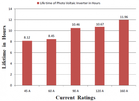
Figure 15. Life Time VS Current Rating
From the above results, it can be concluded that the life span of the photo voltaic inverter circuit increases with an increase in the current ratings of the IGBT. This is due to a decrease in losses and junction temperature of an IGBT.
This paper describes the PV inverter reliability and performance under several current ratings that have been specified, the effect of junction temperature on lifetime is studied, and relevant lifetime is estimated. It has been proven that switching devices rated at different nominal currents have shown unequal thermal performances, leading to varied lifetime performances. The electro thermal modelling of power semiconductor modules has been thoroughly explained. The power loss modelling is based on look-up tables provided by the manufacturers in the datasheet that can be implemented in the PLECS Blockset in the Simulink environment so that the instantaneous switching and conduction losses can be calculated. On the other hand, the thermal modelling is based on a thermal equivalent network named the Foster model, whose parameters are also provided in the data sheets. For this study, the heat sink will be considered for each IGBT solution; it should be noted that an extended approach is to introduce the design variable of the heat sink parameter so the total cost of IGBT modules and cooling system can be considered. However, due to the constrained time frame, it is not included. Therefore, the PV inverter designers can choose the most reliable IGRT by this procedure.
|
MTTF - |
Mean Time To Failure |
|
MTTR - |
Mean Time To Repair |
|
MTBF - |
Mean Time Between Failures |
|
IGBT - |
Insulate Gate Bipolar Transistor |
|
EOL - |
End Of Life |
|
PCT - |
Power Cycle Test |
[1] Alavi, O.; Hooshmand Viki, A.; Shamlou, S. A Comparative Reliability Study of Three Fundamental Multilevel Inverters Using Two Different Approaches. Electronics 2016, 5, 18. https://doi.org/10.3390/electronics5020018
[2] P. Zhang, Y. Wang, W. Xiao and W. Li, "Reliability Evaluation of Grid-Connected Photovoltaic Power Systems," in IEEE Transactions on Sustainable Energy, vol. 3, no. 3, pp. 379-389, July 2012, doi:10.1109/TSTE.2012.2186644.
[3] Kumar, D.G., Bhoopal, N., Ganesh, A., Sireesha, N.V., Rao, D.S.N.M. (2023). Implementation of an asymmetric multilevel inverter for solar photovoltaic applications using N-R approach. Journal of New Materials for Electrochemical Systems, Vol. 26, No. 1, pp. 7-17. https://doi.org/10.14447/jnmes.v26i1.a02
[4] R. A. Minamisawa, U. Vemulapati, A. Mihaila, C. Papadopoulos and M. Rahimo, "Current Sharing Behavior in Si IGBT and SiC MOSFET Cross-Switch Hybrid," in IEEE Electron Device Letters, vol. 37, no. 9, pp. 1178- 1180, Sept. 2016. doi:10.1109/LED.2016.2596302.
[5] H. Wang et al., "Transitioning to Physics-of-Failure as a Reliability Driver in Power Electronics," in IEEE Journal of Emerging and Selected Topics in Power Electronics, vol. 2, no. 1, pp. 97-114, March 2014, doi:10.1109/JESTPE.2013.2290282.
[6] L. Amber and K. Haddad, "Hybrid Si IGBT-SiC Schottky diode modules for medium to high power applications," 2017 IEEE Applied Power Electronics Conference and Exposition (APEC), Tampa, FL, USA, 2017, pp. 3027-3032, doi:10.1109/APEC.2017.7931127.
[7] Feng, Z.; Zhang, X.; Wang, J.; Yu, S. A High- Efficiency Three-Level ANPC Inverter Based on Hybrid SiC and Si Devices. Energies 2020, 13, 1159. https://doi.org/10.3390/en13051159.
[8] S. Singh Kshatri, J. Dhillon and S. Mishra, "Impact of Panel Degradation Rate and Oversizing on PV Inverter Reliability," 2021 4th Int’l Conference on Recent Developments in Control, Automation & Power Engineering (RDCAPE), 2021, pp. 137-141, doi:10.1109/RDCAPE52977.2021.9633585.
[9] Kumar, D.G., Sireesha, N.V., Rao, D.S.N.M., Kasireddy, I., Narukullapati, B.K., Gatla, R.K., Babu, P.C., Saravanan, S. (2023). Modelling of symmetric switched capacitor multilevel Inverter for high power appliances. Journal of New Materials for Electrochemical Systems, Vol. 26, No. 1, pp. 18-25. https://doi.org/10.14447/jnmes.v26i1.a03
[10] C. Liu et al., "Hybrid SiC-Si DC–AC Topology: SHEPWM Si-IGBT Master Unit Handling High Power Integrated with Partial-Power SiC-MOSFET Slave Unit Improving Performance," in IEEE Transactions on Power Electronics, vol. 37, no. 3, pp. 3085-3098, March 2022, doi:10.1109/TPEL.2021.3114322.
[11] Gatla, R.K., Kshatri, S.S., Sridhar, P., Malleswararao, D.S., Kumar, D.G., Kumar, A.S., Lu, J.H. (2022). Impact of mission profile on reliability of gridconnected photovoltaic inverter. Journal Européen des Systèmes Automatisés, Vol. 55, No. 1, pp. 119-124. https://doi.org/10.18280/jesa.550112.
[12] Kumar, D.G.; Ganesh, A.; Sireesha, N.V.; Kshatri, S.S.; Mishra, S.; Sharma, N.K.; Bajaj, M.; Kotb, H.; Milyani, A.H.; Azhari, A.A. Performance Analysis of an Optimized Asymmetric Multilevel Inverter on Grid Connected SPV System. Energies 2022, 15, 7665. https://doi.org/10.3390/en15207665.
[13] Kshatri, S.S., Sireesha, N.V., Rao, D.S.N.M., Gatla, R.K., Kumar, T.K., Babu, P.C., Saravanan, S., Bhoopal, N., Kumar, D.G. (2023). Reliability assessment of hybrid silicon-silicon carbide IGBT implemented on an inverter for photo voltaic applications. Journal of New Materials for Electrochemical Systems, Vol. 26, No.1, pp. 1-6. https://doi.org/10.14447/jnmes.v26i1.a0.
[14] Myla, A.K., Gorantla, S.R. (2023). Performance analysis of balanced integrated standalone microgrid under dynamic load conditions. Journal of New Materials for Electrochemical Systems, Vol. 26, No. 3, pp. 155-163. https://doi.org/10.14447/jnmes.v26i3.a03
[15] Ranjith Kumar Gatla, Guorong Zhu, Jianghua Lu, Sainadh Singh Kshatri, Gireesh Kumar Devineni, The impact of mission profile on system level reliability of cascaded H-bridge multilevel PV inverter, Microelectronics Reliability, Volume 138, 2022, 114639, ISSN 0026-2714, https://doi.org/10.1016/j.microrel.2022.114639.
[16] S. Bouguerra, M. R. Yaiche, O. Gassab, A. Sangwongwanich and F. Blaabjerg, "The Impact of PV Panel Positioning and Degradation on the PV Inverter Lifetime and Reliability," in IEEE Journal of Emerging and Selected Topics in Power Electronics, vol. 9, no. 3, pp. 3114-3126, June 2021, doi: 10.1109/JESTPE.2020.3006267.