Kaustubh G. Kulkarni* | Sanjay N. Havaldar
© 2023 IIETA. This article is published by IIETA and is licensed under the CC BY 4.0 license (http://creativecommons.org/licenses/by/4.0/).
OPEN ACCESS
In a solar power plant, the circular central solar receiver aids in the segregation of electricity output. Because the geometry of the receiver has different diameters in existing approaches, which determines the exact reaction of the fluid on a whole is quite challenging. The mathematical design and modeling of a solar central receiver with a variable diameter header are discussed in this research paper. Hence, a novel Thermo-Mechanical Joint Behavior Analyzing CFD model is employed to solve large-scale transient fluctuation activities directly, while a sub-grid-scale model is used to compute small-scale motions implicitly using Navier-Stokes equations. Moreover, the joints are very vital influences for losses and creation of pressure so there is a high need to analyze the joint efficiently. Consequently, the joints are an essential part of the header which influences more to the performance of the solar receiver, thereby the experimentation is carried out for measurement of pressure difference, turbulence, velocity distribution due to the movement of a Nano-fluid medium in the solar convergent-divergent header configuration precisely.
solar central receiver, computational fluid dynamics, mathematical modeling, mechanics of joint, joint elements
CSP (concentrated solar power) is a cutting-edge renewable energy conservation approach. Solar energy has been recognized a one of the providential renewable energy technologies. CSP (long wave range) or PV (short wave range) technologies [1]. At the present time the solar energy the most reliable alternative energy source; however, it cannot be used to create electricity directly owing to its low intensity. By constructing the suitable concentrating systems, it may be used for a far reaching of energy input devices, from domestic to industrial use [2]. Solar energy can be converted directly from the Photovoltaic systems into electricity, which can then be stored in batteries for later use. Both technologies have progressed in diverse ways since a solar energy first arrived in the renewable energy market in the 1970s. PV plants have discovered a way to cut down the costs by seeking more energy-efficient and cost-effective solar cells, allowing for quicker plant- drive times and installation [3].
Another type of solar system gathers solar energy and transmits it to a working fluid by sensible heating of a fluid that continuously passes through tubes. Solar collectors, also known as central solar receivers, are a renewable technology that collects solar radiation and converts it into hightemperature thermal energy for chemical processing and electricity production. Flat plate solar collectors (FPSCs) are the most basic form of collector because they are simple to build, affordable, and low-maintenance [4].
There are several parameters that have a functional link with the thermal efficiency of a solar collector. Collection plate position, coating substance, collector plate coating, glazing material quality, riser tube diameter spacing, flow velocity, incoming radiation intensity, and bottom and side insulation thickness are all factors to consider. Working fluid improves the performance of solar collectors [5]. Nano fluids are cutting-edge working fluids that are attracting a lot of attention from researchers across the world as a method to increase the efficiency of energy absorption and transport systems. To ensure system compatibility, design change is a thorough strategy that influences a wide variety of other properties. The continual and systematic contributions of researchers from all around the world have enabled engineering and technological breakthroughs in FPSC [6]. A solar central receiver (SCR), also known as a solar power tower, powers a traditional steam Rankine cycle and is one of the most common designs for CSP systems. There have been various studies on this design, with several design focusing on economic assessments and thermodynamic [7]. Consequently, to make the key components worthy of their allotted job, modifications in design are always followed by changes in new mechanics, techniques, and even changes in working fluid. In terms of spiral tube collectors, the one used in (S.K. Verma et al) study is novel [8]. Computational Fluid Dynamics (CFD) is a subfield of fluid dynamics that is abbreviated as CFD. The development of high-performance computer hardware, as well as the advent of user-friendly interfaces, has prepared the way for widespread use of CFD in a variety of sectors [9] [10]. Aerodynamics of aircraft and vehicles (improving the mixing capability of a static mixer for use in wastewater treatment or refineries in the oil and gas market), chemical process engineering (improving the mixing capability of a static mixer for use in wastewater treatment or refineries in the oil and gas market), biomedical engineering, and drying technology are examples of such fields [11-14].
The contribution of this paper,
Thermo-Mechanical Joint Behavior Analyzing CFD model is used to directly solve large-scale transient fluctuation activities, whereas a sub grid scale model is employed to implicitly estimate small-scale movements using NavierStokes equations.
To measure the pressure difference, the joints are evaluated at five separate segments: maximum diameter junction, minimum diameter junction, average diameter junction, and both inlet and outflow, thereby ensuring thermal behavior of the panel.
The reminder of the paper has been ordered as follows: section 2 presents the recent literatures; section 3 depicts the detail description of the anticipated methodology; section 4 discusses the implementation results; finally, section 5 concludes the paper.
Wang et al [15] The fluid, thermal and mechanical properties of the S-CO2 tubular receiver panel under nonuniform solar light distribution are quantitatively investigated utilizing S-CO2 as the heat transfer fluid. Also discussed is the effect of solar flux distribution and flow patterns on thermal and mechanical performance. The findings show that the nonuniform solar flux of the receiver panel increases thermal loss and stress. Laporte et al [16] The influence of design and time resolution on the predicted lifetime of a solar power tower's molten-salt external tubular receiver, one of the most spoiled components of these facilities, is examined in this research, which considers operation under clear circumstances. Where, the heliostat field targeting technique is determined first, and operating limits of the receiver are adjusted to maintain a insufficient film temperature and prevent the stress reset. The former stops the tubes from corroding too quickly, while the latter ensures global stress relaxation, which greatly minimizes the risk of damage during receiver cycle operation.
Fang et al [17] the solar cavity receiver's thermal and mechanical performance as the physical model for this research A superheated water/steam solar cavity receiver with three boiling panels served as the physical model. An integrated simulation method which combines the MonteCarlo ray tracing (MCRT) method, the finite volume method (FVM), the appropriate heat transfer correlations, and the finite element method was used to provoke the complicated heat transfer process inside the receiver and the thermal stress investigation for the absorber panels (FEM) conducted.
Garbrecht et al [18], The thermal efficiency of a molten salt solar central receiver was examined. The novel receiver for a heliostat field around it, is made up of several hexagonal pyramid-shaped parts grouped alveolar with their apexes pointing at the heliostats. On the outside, concentrated solar energy is absorbed, while on the inside, a molten salt flow cools the components. The arrangement can nearly be termed a radiation trap because most of the radiative losses are reabsorbed by the nearby pyramids. As a result, the efficiency of the novel receiver was examined using coupled CFDsimulations for radiation and heat transmission into the molten salt flow. Assuming a focused incident power of 1 MW/m2 attained 91.2 percent thermal efficiency. Therefore, loss caused by reflection could be compact to 1.3% of incoming radiation, while it losses by emission accounted for 2.8%.
Craig et al [19], A Computational Fluid Dynamics (CFD) model is created of the solar receiver cavity. The innovative receiver is made up of multiple hexagonal pyramid-shaped components clustered alveolar with their apexes pointing at the heliostats and is designed to receive a heliostat field surrounding it. Concentrated solar energy is absorbed on the exterior, while a molten salt flow cools the components on the inside. Because most of the radiative losses are re-absorbed by the neighboring pyramids, the configuration is almost a radiation trap. As a consequence, utilizing coupled CFDsimulations for radiation and heat transmission into the molten salt flow, the efficiency of the new receiver was investigated. A 91.2 percent thermal efficiency was achieved using a focused incident power of 1 MW/m2. As a result, losses due to reflection could be limited to 1.3 percent of incoming radiation, while losses due to emission accounted for the remainder.
Baretto et al [20], addressed the Computational Fluid Dynamics (CFD) modelling and thermal performance analysis of porous volumetric receivers accompanied to solar concentration systems. The heat transfers and fluid flow processes in porous media are also modelled using volume averaged mass, and energy conservation equations and momentum, with the local thermal non-equilibrium (LTNE) approach, thermal radiation transfer is described using the P1 spherical harmonics method, with open-source software (Open FOAM). To describe the transmission and absorption of solar light, an in-house algorithm based on the Monte Carlo Ray Tracing (MCRT) approach was created and connected to the CFD mesh. This reference configuration's thermal power output, mean fluid temperature at outlet, thermal efficiency, mean fluid temperature at outlet, and pressure drop are 628.92 W, 85.46 percent, 474.22 K, and 103.10 Pa respectively. As a result, using receivers with large porosity and pores reduces pressure while increasing thermal efficiency marginally.
Digole et al [21], To study the change of heat transfer characteristics of fluid and temperature within the receiver an external receiver was designed, manufactured and experimentally evaluated by the concentrated central receiver system. The exit temperature of the water was determined using steady-state numerical simulation using ANSYS Fluent. The experimental data were used to demonstrate the CFD results. As a result, the fluid temperature changed according to the number of heliostats and the mass flow rate. At solar noon, nine heliostats with a mass flow rate of 0.0016 kg/sec achieved a maximum temperature of 92.4°C, with an average temperature of 84.4°C for the whole day. As a result, the spiral coil tube's heat transfer coefficient and pressure drop were 1.44 and 1.97 times greater than the straight tube's.
Nidhul et al [22], Computational fluid dynamics (CFD) and energy analysis are displayed to investigate the impact of secondary flow produced by V-ribs on the overall performance of a triangular solar air heater (SAH) duct. The influence of rib inclination is deliberated using CFD approach for various Reynolds number (5000 Re 20000) with a given relative rib height (Rh = 0.05) and relative rib pitch (Rp=10). Empirical correlations is capable of predicting Nu and f with an absolute variance of 8.7% and 4.7 percent, respectively. It is created based on the CFD simulation findings. As a result of the exergy study, the ribbed triangular duct generates less entropy than the smooth duct, with a maximum increase in energetic efficiency (ex) of 23 percent for = 45°. Comprehensive study to compare the performance of the rectangular duct to that of the ribbed triangle duct SAH is equal to 45°. The results demonstrate that the ribbed triangle duct SAH (= 45°) is better to other ribbed rectangular duct configurations. Said et al [23], Endothermic reactions, namely methane reforming, can be obsessed using parabolic trough solar collectors and molten salts as heat transfer fluid. On the other hand, Linear focus concentrators can only offer temperatures below 600 C, resulting in CH4 conversions much below 50%. The equilibrium can be altered toward significantly higher conversations, if H2 is continuously withdrawn from the reaction mixture using an H2-selective membrane while simultaneously generating a higher purity of H2 stream. A molten salt and tube heated packed bed membrane reformer is numerically evaluated in this study utilizing computational fluid dynamics and non-isothermal formulation.
From Survey, [15] The thermal, fluid, and mechanical properties of the S-CO2 tubular receiver panel are investigated using S-CO2 as the heat transfer fluid. [16] Also the design day on the estimated lifetime and the impact of time resolution of a solar power tower's molten-salt external tubular receiver, which is one of these facilities' most damaged components. [17] The radiative losses are absorbed by the neighboring pyramids in a thermal stress analysis [18], and the geometry is parameterized to allow the selection of design variables in a formal design optimization formulation [19]. [20] Using receivers with low porosity and pore size reduces thermal efficiency somewhat while significantly increasing pressure loss. [21] The fluid temperature was precise by the number of heliostats and the mass flow rate. The exergy analysis presented by [22] demonstrates that the entropy created by the ribbed triangular duct with least efficiency is lower. [23] Linear focus concentrators, on the other hand, can only provide temperatures below 600 C. As a result, a unique topology must be implemented to address the aforementioned concerns.
Renewable energy conservation technology is critical for preserving renewable energy and converting it to a usable form where the CFD program is used to model the flow of fluid at the header receiver's gradual convergence and gradual divergence junctions using reported flow parameters at the junctions and to examine the thermal stress concentration caused by fluid flow. Because the design of the receiver has different diameters, determining the exact response of the fluid as a whole is quite challenging. To overcome the abovementioned issue a novel Thermomechanical joint behavior analyzing CFD model has been proposed in which the NavierStokes equations are employed directly to solve large-scale transient fluctuation movements, while a sub-grid-scale model is used implicitly to compute small-scale motions. Furthermore, the joints are an important component of the header that has a greater impact on the functioning of the solar receiver and hence, the joints are examined at five different sections: maximum diameter junction, minimum diameter junction, average diameter junction, and inlet and outflow. The velocity distribution is computed using Bernoulli's theorem, Turbulence with k-epsilon model, wall-adapting local eddyviscosity model, and the transition from laminar to turbulence. The most important component in determining the behavior of the solar receiver is thermal behavior of the panel. Additionally, the temperature is altered to various values, and the thermal concentration is determined at the five joints.
Figure 1. Block diagram of the proposed Thermo mechanical joint behavior
The mechanical characteristics that alter as a function of the thermal behavior are also thoroughly examined. The block diagram of the proposed methodology is depicted in Figure 1.
3.1 Thermo mechanical joint behavior analyzing CFD model
Thermo-Mechanical Joint Behavior Analyzing CFD model is used to analyse the circular header receiver with varied diameter for its performance under various conditions. The Navier-Stokes equations are used to solve large-scale transient fluctuation movements, while a sub grid size model is used to compute small-scale motions implicitly. As a result, the parallel plate model is widely practiced to determine the fracture permeability m, which was derived by applying the Navier—Stokes equation to laminar incompressible flow between two parallel smooth plates. The hydraulic aperture, which is the joint's effective opening to fluid flow, is also depicted as a function of its permeability. The hydraulic aperture of the fracture does not match its mechanical aperture because actual fractures deviate substantially from ideal parallel plates.
$m=\frac{e_i{ }^2}{12}$ (1)
where, $e_i \rightarrow$ Hydraulic aperture of the joint.
To estimate the hydraulic aperture from the mechanical aperture, the following empirical connection is shown in Eq. (2).
$e_i=\frac{e_n^2}{J R C}$ (2)
where, JRC→ Joint roughness coefficients.
$e_i$ and $e_n$ are in $\mu m \rightarrow$ Mechanical aperture of the joint. In addition, a linear link between mechanical apertures and hydraulic are shown in Eq. (3).
$e_i=e_{i 0}+g \Delta e_n$ (3)
where, $e_{i 0}$ is the initial hydraulic aperture, $\Delta e_n$ is the variation in mechanical aperture owing to the combined effects of compression and shear, and g is a proportionality factor. When, g ranges between 0.5 to 1. The roughness of the joint surfaces contributes to this component. The limiting ideal case of parallel smooth plates has a factor g=1, this circumstance exists only when the joint is relatively open, with apertures of the order of mm are shown in Eq. (4). In the majority of other circumstances, $g<1$ the shape of the flow path has a significant influence on g. Where, g is often close to 0.8 for rectilinear laminar flow.
$g=g_{0 \exp }\left.\left(-\int_0^{u^q} d_g d u^q\right)\right.$ (4)
where, $d_g$ is a production gauge factor. Where, the additional parameters $g_0$ and $d_g$ presented in this section are extremely likely to be experimentally connected to JRC, JCS, and q. To get to specific correlations, a detailed experimental design will be required.
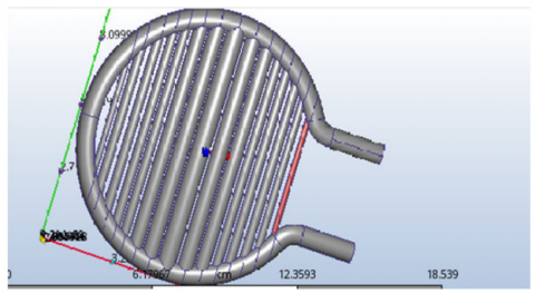
Figure 2. Design of Thermomechanical joint behaviour using CFD model
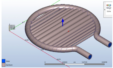
Autodesk CFD was used to simulate the solar central receiver with thermo-mechanical joint behavior. The diameter of the upper header inlet and outlet is 15 mm and 50 mm and the diameter of the bottom header inlet and outlet is 15 mm and 50 mm, the diameter of the upper header inlet and outlet is 15 mm and 50 mm, the number of tubes is 15, the area of the receiver is 0.6 m2, the heat flux is 3500 w/m2, and the material of the receiver and frame is copper. Also, the simulation fluid is water, which has a constant density of 997 kg/m3 and a dynamic viscosity of 0.0008 kg/ms are shown in Figure 2. The fluid is assumed to be incompressible, with mass flow at the input and pressure at the output chosen as the boundary conditions. Hence, the experimental procedure is explained in the below subsection.
3.2 Experimental procedure
The joints are an important component of the header that has a greater impact on the functioning of the solar receiver. Hence, the joints are examined at five different sections: maximum diameter junction, minimum diameter junction, average diameter junction, and inlet and outflow.
Figure 3. Circular solar receiver
The following procedures were taken throughout the testing method to investigate the influence of outlet inclination on the phase split:
The outlet branches were angled as required.
The suitable air inlet control valve was changed to provide the necessary air inlet flow rate. Therefore, the necessary air outlet control valves were simultaneously adjusted to achieve the target junction pressure of 2.0 atm (abs).
The water pump was twisted on when the suitable water inflow rotameter valve was entirely opened where, the flow rate was set by adjusting the control valve.
The right test section the pressure of 2.0 atm (abs) was conserved by continually changing the air control valves. The water level in the separation tanks was kept constant by managing the exit water flow rates via valves. The exact test conditions of test section pressure, correct extraction ratio, input flow rate and constant water level in the separation tanks necessitated this repeating technique.
The mass split ratio (W3/W1) was evaluated with the appropriate test section pressure, intended intake flow rate, and a stable level of liquid in the separation tanks. If it differed from the required value, the air control valves downstream from the separation tanks were used to correct it. Also, the mass split ratio was adjusted in such a way that the right intake mass flow rate and pressure were maintained. Iterative procedures were used until the required operational conditions were totally met.
The quantity of period required to alter the flow variables in the loop was resolute by the intake flow conditions and the value of the mass split ratio (W3/W1). Before capturing any phase distribution data during the steady-state period, the following parameters required to remain fixed:
The pressure at the intersection (Ps).
The water and air mass flow rates at the inlet and outlet.
The water level in the filter tanks.
The air and water pressures and temperatures throughout the system. By, using the required parameters of WG1, WL1, WG2, WL2, WG3, and WL3, the following criteria were calculated.
$W_j=W_{H j}+W_{M j} \quad j=1,2, \ldots n$ (5)
The inlet and the outlet qualities were calculated by,
$y_j=\frac{W_{H j}}{W_i} \quad j=1,2 \ldots . n$
where, W be the mass flow rate $\left(K g s^{-1}\right)$
H be the gravitational acceleration
M be the liquid
j be the superficial velocity $\left(\mathrm{ms}^{-1}\right)$
y be the quality
Therefore, the fraction of total inlet liquid entering outlet and the fraction of total inlet gas entering outlet were calculated using above equations.
A beam problem may be reduced to a simple harmonic oscillator differential equation retaining linear material features hypothesis and eigenvalues solution because of structural dynamic theory. Hence, bending deformations are examined when the Euler-Bernoulli hypothesis is used. All of these hypotheses lead to a set of equations corresponding to an equivalent damped harmonic oscillator solution for each Eigen mode.
$N_{e q}=\int N \overline{V^2} d V$ (6)
$K_{e q}=\int F J\left(\frac{d^2 \bar{V}}{d y^2}\right)^2 d V$ (7)
$H_{e q}=\int H \bar{V} d V, \omega=\sqrt{\frac{K_{e q}}{N_{e q}}}$ (8)
Assuming statistical independence of the forces at each ring, the equivalent force term may be defined as square sum. This model provides an estimate of the supreme movement of the rods, allowing users to determine whether moving frame simulations are required are shown in table 1.
Table 1. Dimensions of proposed experimental setup
|
S.NO |
Parameters |
Dimensions |
|
1 |
Diameter of Bottom Header Inlet and Outlet |
50mm and 15 mm |
|
2 |
Diameter of Upper Header Inlet and Outlet |
15mm and 50mm |
|
3 |
Area of receiver |
0.6m2 |
|
4 |
No of Tubes |
15 |
|
5 |
Diameter of central tube |
50mm |
|
6 |
Tube Thickness |
1mm |
|
7 |
Mass Flow Rate |
0.1LPM |
|
8 |
Heat Flux |
3500w/m2 |
|
9 |
Metal halide lamps (solar simulator) |
3-4 qty. (1000W) |
|
10 |
Material of Receiver & Frame |
Copper – Receiver |
Thus the velocity distribution is determined via wall adapting eddy viscosity and k-epsilon turbulence model is explained in the below section.
3.2.1 Turbulence and velocity distribution model
The K-epsilon $(\mathrm{k}-\varepsilon)$ turbulence model is the most frequently used model in computational fluid dynamics (CFD) to simulate mean flow characteristics under turbulent flow conditions. It is a two-equation model that uses two transport equations to provide a broad characterization of turbulence (partial differential equations, or PDEs). The K-epsilon model was created to improvise the mixing-length model to provide an alternative to algebraically dictating turbulent length scales in moderate to high-complexity flows.
The velocity is parted into a mean flow component and a fluctuating component with a zero temporal average because of the Reynolds decomposition. As a consequence, the Reynolds Stress terms $u_i u_j$ have a closure issue. For algebraic models, the $u_i u_j$ are supposed isotropic, so that all of the tensor cross components may be attributed to the generation and dissipation of turbulent kinetic energy. A kinetic turbulence energy balance equation and a dissipation rate equation are derived from this assumption. In addition, the turbulent eddy viscosity $\mu_t$ is the ratio using a simple algebraic equation the relationship between kinetic turbulent energy and dissipation rate are shown in Eqs. (9) and (10).
For turbulent kinetic energy,
$\frac{\partial(\rho l)}{\partial t}+\frac{\partial \rho u_i}{\partial x_i}=\frac{\partial}{\partial x_j}\left[\frac{u_t}{\sigma_k} \frac{\partial l}{\partial x_j}\right]+2 \mu_t F_{i j}^2-P \varepsilon$ (9)
For dissipation,
$\frac{(\partial P \varepsilon)}{\partial t}+\frac{\partial\left(P \varepsilon u_i\right)}{\partial x_i}=\frac{\partial}{\partial x_j}\left[\frac{\mu_t}{\sigma \varepsilon} \cdot \frac{\partial \varepsilon}{\partial x_j}\right]+D_1 \varepsilon \frac{\varepsilon}{l} 2 \mu_t F_{i j}^2-D 2 \varepsilon \rho \frac{\varepsilon^2}{l}$ (10)
Where, $u_i$ denotes the component of velocity in the relevant direction.
$F_{i j}$ denotes a rate of deformation component.
$\mu_t$ denotes the eddy viscosity.
$\mu_t=\rho D_\mu \frac{l^2}{\varepsilon}$ (11)
$\sigma_k, \sigma_{\varepsilon}, C_{1 \varepsilon}$ and $C_{2 \varepsilon}$ are constants. Thus the pressure difference is mentioned via Bernoulli’s model are explained in the below subsection.
3.2.2 Pressure difference model
Bernoulli's principle of fluid dynamics circumstances i.e. an increase in fluid speed occurs simultaneously with a decrease in static pressure or potential energy. As a consequence, fluid particles are simply impacted by their own weight and pressure. If a fluid is flowing horizontally along a section of a streamline, it can only increase in speed because the fluid has moved from a higher pressure region to a lower pressure region and it can only decrease in speed because the fluid has moved from a lower pressure region to a higher pressure region. the quickest speed occurs where the pressure is lowest, and th e slowest speed occurs at pressure is highest in a horizontally flowing fluid. In most cases gases and liquids flowing at low Mach numbers, the density of a fluid packet may be considered to remain constant, regardless of pressure variations in the flow. As a result, the fluid can be termed incompressible, and incompressible flows are the outcome. The following is a common variation of Bernoulli's equation that may be used at any point along a streamline:
$\frac{w^2}{2}+h z+\frac{p}{\rho}=Constant $ (12)
where, w denotes the velocity of fluid flow at a location on a streamline.
h be the acceleration due to gravity.
z be the Elevation of a point above a reference plane, with the positive z-direction pointing upward - that is, in the opposite direction of gravitational acceleration.
p be the pressure at the particular point.
For this Bernoulli equation to operate, the assumptions are followed.
The flow is stable, which means that the flow characteristics (velocity, density, and so on) at any point cannot fluctuate over time. The flow is incompressible i.e., even if pressure fluctuates, the density must remain constant along a streamline. Also, viscous force friction is to be minimal.
Bernoulli's equation may be generalized to conservative force fields as follows:
$\frac{w^2}{2}+\varphi+\frac{p}{\rho}=Constant $ (13)
where, $\varphi$ be the force potential at the location on the streamline under consideration. $\varphi=h x$
Equation (12) may be expressed as follows by multiplying by the fluid density:
$\frac{1}{2} \rho w^2+\rho h x+p=$ constant (14)
(or) $\quad q+\rho h i=p_0+\rho h x=$ constant (15)
where, $q=\frac{1}{2} \rho w^2$ is a dynamic pressure $i=x+\frac{P}{\rho h}$ is a hydraulic head $P_0=P+q$ is a Stagnation pressure The Bernoulli equation's constant can be normalized. A typical method is to express total head or energy head H:
$H=x+\frac{p}{\rho h}+\frac{w^2}{2 h}=i+\frac{w^2}{2 h}$ (16)
According to the preceding equations, Pressure is zero at a certain flow speed, while pressure is negative at higher rates. Bernoulli's equation is plainly no longer valid before zero pressure reached since gases and liquids seldom achieve negative absolute pressure, let alone zero pressure. When the pressure in a liquid drops too low, cavitation occurs. The equations above take use of a linear relationship between pressure and flow speed squared. Higher gas flow rates or sound waves in water liquids, because considerable variations in mass density, making the premise of constant density invalid. Consequently, the temperature is varied to different values and the thermal concentration is defined at the defined five joints. Also the mechanical characteristic changes based on the thermal behavior is also analyzed thoroughly. In this, we have compared our results with CFD software packages with classical formula and made an attempt to analyze the geometrical Configuration. Hence, the experiment is carried out to carefully quantify the pressure differential, turbulence, and velocity distribution caused by the flow of a micro fluid medium in a solar convergent divergent header configuration. The further implementation particulars of the proposed SCR with thermos mechanical joint behavior have been presented in the next section.
This section includes a full discussion of the implementation outcomes as well as the proposed system's assessment measures. A comparison has also been made to show that the suggested models performance outperforms existing models.
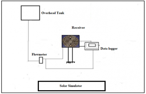
4.1 Experimental Setup
This work has been implemented in the working platform of Autodesk CFD with the following system specification and the simulation results are discussed below.
Platform: Autodesk CFD
OS: Windows 10
Processor: 64-bit Intel processor
RAM: 8 GB
4.2 Simulation outputs
This section presents the simulation outputs and its discussion in detail upon Solar Central Receiver with ThermoMechanical Joint Behavior.
Figure 4. Gradual expansion joints in CFD Analysis
The steady expansion and contraction joints are depicted in different dimensions. Figure 3 show the joint geometries of progressive expansion and contraction.
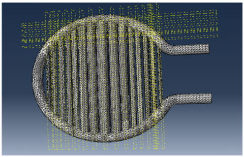
Figure 5. Mesh analysis
The geometry and mesh are made up of a multi-dimensional joint generated by combining the coordinates. For the aforementioned geometry, boundary conditions such as velocity intake and pressure outlet, as well as a fixed wall with no-slip condition, have been implemented are shown in figure 5 and statistically represented in Table 2 and Table 3.
Table 2. Automatic mesh testing
|
Parameters |
Dimensions |
|
Surface |
0 |
|
Gap refinement |
0 |
|
Resolution factor |
1.0 |
|
Edge growth rate |
1.1 |
|
Minimum points |
2 |
|
Points on longest |
10 |
|
Surface limiting |
20 |
Table 3. Mesh enhancement settings
|
Parameters |
Dimensions |
|
Mesh enhancement |
1 |
|
Enhancement blending |
0 |
|
Number of layers |
3 |
|
Layer factor |
0.45 |
|
Layer gradation |
1.05 |
Figure 6. Joints in a Flow-Through Pipe: CFD Analysis
The distribution of all flow variables, primarily flow velocity, at intake borders must be stated in inlet boundary conditions. When the inlet flow velocity is known, this form of boundary condition is commonly employed.Fig.6. is designed using 386121 number of nodes and 1602420 number of elements.
Table 4. Outlet 1 flow through pipe
|
Parameters |
Dimensions |
|
Mass flow out |
-0.0157529 |
|
Minimum x,y,z of |
0.0 |
|
Node near minimum |
681.0 |
|
Outlet bulk pressure |
4000000.0 |
|
Outlet bulk |
-0.0 C |
|
Outlet mach number |
6.23199e-12 |
|
Outlet residence time |
9.32964 sec |
|
Reynolds number |
3.02258 |
|
Surface id |
299.0 |
|
Volume flow out |
-0.0157813 |
The distribution of all flow variables, particularly flow velocity, must be specified in outlet1 and outlet 2 boundary conditions. Consequently, a typical form of boundary condition is given when the outlet velocity is known. When the outlet is selected far away from the geometrical disturbances, the flow reaches a full matured condition with no change in flow direction. In such a region, an outlet could be drawn, and the gradient of all variables in the flow direction, except pressure, could be equal to zero are shown in Table 4 and Table 5.
Table 5. Outlet 2 flow through pipe
|
Parameters |
Dimensions |
|
Mass flow out |
0.0157557 g/s |
|
Minimum x,y,z of opening |
0.0 |
|
Node near minimum x, y, z of opening |
1617.0 |
|
Outlet bulk pressure |
8000000.0 |
|
Outlet bulk |
0.0 C |
|
Outlet mach number |
6.57776e-12 |
|
Outlet residence time |
3.40615e-09 |
|
Reynolds number |
2.97955 |
|
Surface id |
298.0 |
|
Total mass flow out |
2.83685e-06 |
|
Total vol. flow out |
2.84196e-06 |
|
Volume flow out |
0.0157841 |
Figure 7. Velocity distribution
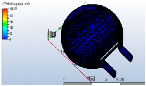
The velocity of flow in a pipe with an input diameter of 12.5 mm and an output diameter of 25 mm. Whether the flow is laminar or turbulent determines the form of the velocity curve (the velocity profile throughout any given piece of pipe). Also, the entire fluid flows at a single value in turbulent flow because the velocity distribution is fairly flat across the pipe segment. Hence, the color contours depict the velocity of an expanding pipe decreases at the entry edges, resulting in velocity loss in the pipe are shown in figure 7.
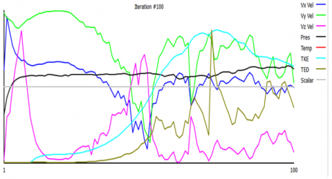
Figure 8. Residuals graph of Iteration#100
The residual is the basic measures of convergence in an iterative solution since it directly quantifies the error in the system of equations solution. Also, the residual measures the local imbalance of a conserved variable in each control volume in a CFD analysis at 100th iteration are shown in figure 8.
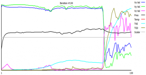
Figure 9. Residuals graph of Iteration#130
The residual in a CFD analysis represents the local imbalance of a conserved variable in each control volume. Also, the residual in an iterative numerical solution will never be zero. Hence, the solution will be more numerically accurate if the residual value is lower at Iteration #130 are shown in figure 9.
Figure 10. Temperature vs concentration ratio at an average beam solar radiation at 800 W/m2
The fluctuation of the optimal receiver surface temperature throughout the geometric concentration ratios is seen in Figure 10. The average beam radiation taken into account is 800 W/m2. The optimal temperature is the nominal for the chosen test location, and the collector takes the ambient circumstances into consideration. When a function of concentration ratio is 100, the temperature is 450 degrees Celsius. When the concentration ratio is 200, the temperature increases to 500 degrees Celsius. When the concentration ratio moves to 400, the temperature gradually rises to 600 degrees Celsius. The overall increase in temperature based on concentration factor at the solar central receiver is calculated as 18% of growth.
4.3 Comparison analysis
In this section, various performances of the proposed Solar Central Receiver with Thermo-Mechanical Joint Behavior Analyzing CFD model have been compared with the existing models to ensure the performance of the proposed model.
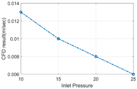
Figure 11. CFD result (m/sec) vs inlet pressure
Pressure intake and outlet conditions are frequently assigned at the opposite end of the model to a flow rate or a different pressure in computational fluid dynamic analysis (CFD). The CFD findings drop when the pressure is increased. At pressure 10, the computational fluid dynamics is 0.013 m/sec, whereas at pressure 15, it is 0.008m/sec are shown in figure 10.
Table 6. Comparison of CFD result(m/sec)
|
Inlet Pressure |
CFD Result (m/sec) |
|
10 |
0.013 |
|
15 |
0.01 |
|
20 |
0.008 |
|
25 |
0.006 |
Figure 12. Outlet velocity (m/sec) vs inlet pressure
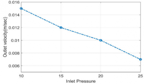
Inlet pressure are calculated rather than fixed when pressure gradients are lowered to zero. As a consequence, for incompressible flows, the temperature characteristics are not required, but the temperature at the input must be specified. Because the turbulent flow amounts are matched to the starting state values, they aren't needed as inputs. In addition, the static (gauge) pressure will be determined based on the velocity profile at the exit to achieve the desired value. Also, the outflow boundary conditions are used to estimate all important scalar values from the interior, with gradients set to zero. When a function, as the inlet pressure rises, the output velocity decreases. Its output velocity is 0.012 m /sec at inlet pressure 15, 0.01 m/s at inlet pressure 20, and 0.008 meters per second at inlet pressure 25 are shown in figure 11.
Table 7. Comparison of outlet velocity(m/sec)
|
Inlet Pressure |
Outlet Velocity (m/sec) |
|
10 |
0.015 |
|
15 |
0.012 |
|
20 |
0.01 |
|
25 |
0.007 |
Figure 13. Inlet velocity (m/sec) vs inlet pressure
The inlet velocity reduces as the inlet pressure rises from 10 to 25, where the output pressure will be slightly higher than the intake pressure in that case (due to flow resistance) are shown in figure.12. The outlet velocity at intake pressure 10 is 2m/sec, whereas at inlet pressure 20, the outlet velocity is 1.5m/sec. Also, friction in the pipe causes the outlet pressure to rise when the outlet pipe is tiny in proportion to the flow rate. When the outlet is directed uphill, the outlet pressure rises with it.
Table 8. Comparison of inlet velocity (m/sec)
|
Inlet Pressure |
Inlet Velocity (m/sec) |
|
10 |
0.002 |
|
15 |
0.0018 |
|
20 |
0.0015 |
|
25 |
0.0014 |
Figure 14. Discharge (Q) vs inlet pressure
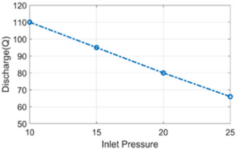
Inlet pressure, often known as pump intake pressure, is the pressure available where the suction pipe meets the booster pump. The inlet pressure is determined by the pressure of the water supply or the water pressure created by the booster if the booster draws from a break tank. Consequently, the centrifugal pump discharge pressure is the total pressure energy after the liquid has passed through the centrifugal pump. Also, as the pressure rises from 10 to 25, Figure 13. shows that at pressure 10, the discharge is 110, and at inlet pressure 20, the discharge is 80.
Table 9. Comparison of discharge (Q) at different Inlet pressure
|
Inlet Pressure |
Discharge (Q) |
|
10 |
110 |
|
15 |
95 |
|
20 |
80 |
|
25 |
66 |
Figure 15. Error (%) Vs inlet pressure
Inlet pressure, also known as pump intake pressure, is the pressure present where the suction pipe meets the booster pump. In addition, the input pressure is determined by the pressure of the water supply or the water pressure created by the booster if the booster draws from a break tank. The error (percent) diminishes as the intake pressure increases. The error value at pressure 10 is $10 \times 10^{-3}$, and at inlet pressure 25, the error is 5%, as illustrated in figure 14.
Table 10. Comparison of error (%) at different inlet pressure
|
Inlet Pressure |
Discharge (Q) |
|
10 |
110 |
|
15 |
95 |
|
20 |
80 |
|
25 |
66 |
This section introduces and investigates the impact of cylinder computation on the absorber cylinder and gatherer execution. In this research, we intended a circular central solar receiver system with a variable diameter header at the top as well as bottom. Where, solar simulators, circular central solar receiver, and concentrator were used to model the exact configuration of the system. Consequently, the thermal storage technology allows the solar central receiver to function even when the weather is cloudy. During the summer, the systems efficiency is at an all-time high. When the results of the systems accurate modelling are compared to CFD simulations, encouraging results are found. Additionally, the modelling should provide a control system for regulating the mass flow rate of the heat transfer fluid or the number of solar simulators, which examines the solar incident energy over time and confirms that the working fluid does not surpass the supreme temperature of the working fluid. The experimental findings reveal that the anticipated framework exceeds the others in terms of velocity distribution of lowest outlet velocity of 0.008 m/sec, lowest input velocity of 1.4 m/sec, discharge of 66, and error of 0.005 %, respectively and as the temperature progressively increases to 600 degrees Celsius, the concentration ratio increases to 400. It is determined that the whole temperature increase represents an 18% gain at the solar central receiver.
[1] Liu, Ming, et al. (2020). Design of sensible and latent heat thermal energy storage systems for concentrated solar power plants: Thermal performance analysis. Renewable Energy, 151: 1286-1297.
[2] Rabaia, Malek Kamal Hussien, et al. (2021). Environmental impacts of solar energy systems: A review. Science of The Total Environment, 754: 141989.
[3] Palacios, A., et al. (2020). Thermal energy storage technologies for concentrated solar power–A review from a materials perspective. Renewable Energy, 156: 1244-1265.
[4] Verma, Sujit Kumar, et al. (2020). Performance comparison of innovative spiral shaped solar collector design with conventional flat plate solar collector. Energy, 194: 116853.
[5] Elcioglu, Elif Begum, et al. (2020). Nanofluid figure-ofmerits to assess thermal efficiency of a flat plate solar collector. Energy Conversion and Management, 204:112292.
[6] Alam, Tabish, et al. (2021). Performance Augmentation of the Flat Plate Solar Thermal Collector: A Review. Energies, 14(19): 6203.
[7] Ellingwood, Kevin, KasraMohammadi, and Kody Powell. (2020). A novel means to flexibly operate a hybrid concentrated solar power plant and improve operation during non-ideal direct normal irradiation conditions. Energy Conversion and Management, 203: 112275.
[8] Verma, Sujit Kumar, Naveen Kumar Gupta, and DibakarRakshit. (2020). A comprehensive analysis on advances in application of solar collectors considering design, process and working fluid parameters for solar to thermal conversion. Solar Energy, 208: 1114-1150.
[9] Kaustubh Kulkarni et al. (2022). Numerical analysis of central solar receivers with various geometries. International Journal of Heat and Technology, 40 (1), 339-346
[10] Kaustubh Kulkarni et.al. (2022). Numerical analysis of concentrated beam solar circular receiver. International Journal of Heat and Technology, 40 (2),375-382.
[11] Nguyen, T.S and Selvadurai, A.P.S. (1998). A model for coupled mechanical and hydraulic behaviour of a rock joint. International Journal for Numerical and Analytical Methods in Geomechanics, 22(1): 29-48.
[12] Mohamed, M.A., Soliman, H.M and Sims, G.E. (2011). Experimental investigation of two-phase flow splitting in an equal-sided impacting tee junction with inclined outlets. Experimental thermal and fluid science, 35(6): 1193-1201.
[13] Stamou, A and IoannisKatsiris. (2006). Verification of a CFD model for indoor airflow and heat transfer. Building and Environment, 41(9): 1171-1181.
[14] Riahi, Soheila, et al. (2021). Transient Thermomechanical analysis of a shell and tube latent heat thermal energy storage for CSP plants. Applied Thermal Engineering, 196: 117327.
[15] Wang, Kun, et al. (2021). Thermal-fluid-mechanical analysis of tubular solar receiver panels using supercritical CO2 as heat transfer fluid under non-uniform solar flux distribution. Solar Energy, 223: 72-86.
[16] Laporte-Azcué, Marta, et al. (2021). Assessment of the time resolution used to estimate the central solar receiver lifetime. Applied Energy, 301: 117451.
[17] Fang, Jiabin, et al. (2021). Thermal characteristics and thermal stress analysis of a superheated water/steam solar cavity receiver under non-uniform concentrated solar irradiation. Applied Thermal Engineering, 183: 116234.
[18] Garbrecht, Oliver, Faruk Al-Sibai, Reinhold Kneer, and Kai Wieghardt. (2013). CFD-simulation of a new receiver design for a molten salt solar power tower. Solar Energy, 90: 94-106.
[19] Craig, K.J., Gauché, P and Kretzschmar, H. (2014). Optimization of solar tower hybrid pressurized air receiver using CFD and mathematical optimization. Energy Procedia, 49: 324-333.
[20] Barreto, Germilly, Paulo Canhoto, and Manuel CollaresPereira. (2019). Three-dimensional CFD modelling and thermal performance analysis of porous volumetric receivers coupled to solar concentration systems. Applied Energy, 252: 113433.
[21] Digole, Satyavan, P., Mathew Karvinkoppa, and SudarshanSanap. (2020). Thermal analysis of a spiral solar receiver for a small central receiver system: An experimental and numerical investigation. International Journal of Ambient Energy, 1-9.
[22] Nidhul, Kottayat, Sachin Kumar, Ajay Kumar Yadav, and Anish, S. (2020). Enhanced thermo-hydraulic performance in a V-ribbed triangular duct solar air heater: CFD and exergy analysis. Energy, 200: 117448.
[23] Said, Syed, A.M., et al. (2016). Solar molten salt heated membrane reformer for natural gas upgrading and hydrogen generation: A CFD model. Solar Energy, 124:163-176.