OPEN ACCESS
The Petri net, a graphic-based simulation tool, can describe the asynchronous and concurrent behaviors of the system, but fails to fully simulate embedded real-time systems. To solve the problem, this paper introduces the real-time description ability into the colored Petri net model, creating a real-time modelling method for embedded real-time system. The design flow of a general embedded real-time system was explained based on the proposed model. Finally, the model was applied to simulate the multi-function vehicle bus (MVB) controller of train communication network, aiming to satisfy the strict requirements on real-time analysis. The results show that the proposed method can fulfil the strict real-time requirements of the train system. The research findings shed new light on the application of Petri nets and the simulation of embedded real-time systems.
colored Petri net, embedded real-time system, formal modeling, model simulation
The traditional development strategy for embedded systems mainly focuses on the late design and implementation, which involves the determination of hardware and software functions through demand analysis, followed by the selection of hardware and division of software modules. This strategy is still feasible for the design of small-scale embedded systems. In recent years, however, the growing demand for complex and uncertain embedded systems has called for the shift of development focus towards the early phase of system design. In this phase, the main task is to set up a conceptual model of the embedded system based on demand analysis, simulate the model on simulation tools, and verify the system design against the simulation results. Compared with the traditional strategy, the early phase design can clarify the system functions, determine the realizability of the system and identify potential errors in advance. One of the keys to early phase design lies in the modelling method of the embedded system.
A Petri net (Peterson, 2010; Jensen et al., 2007) is a graphical-based mathematical tool that formalizes the asynchronous and concurrent system behaviors. Recently, many advanced Petri nets with strong abstraction and description abilities have been developed, including time Petri net (Berthomieu and Diaz, 1991) and colored Petri net (Liu et al., 2002). The emergence of advanced Petri nets provides a rigorous, efficient and usable modeling and analysis method for embedded, distributed and highly reliable systems. Nevertheless, these advanced Petri nets fall short in the modelling and analysis of embedded real-time systems. For instance, time Petri net cannot effectively analyze the randomness of transition delay, neither can colored Petri net give an explicit description of the system’s time.
In view of the above, this paper explores the modelling and design method of colored Petri net based on exact semantics, puts forward a real-time colored Petri net model, and, on this basis, designs a real-time analysis method. The method supports full description of the function and time attributes of embedded real-time systems, and applies to the design of highly secure and reliable real-time systems.
Much research has been done on embedded system development at home and abroad. For example, Chen et al. (2001) created an embedded system modelling method based on Unified Modeling Language (UML). This object-oriented method divides the embedded system into several modular objects, and depicts the structure and function of each object by class, marking and collaboration diagrams. In this way, certain features of the embedded system can be described with high accuracy. Rettberg (2015) suggested modelling embedded systems by program state machine. Taking behavior as the object, this modelling strategy manages to provide a clear description of the system and represent the system as an intuitive equivalent graph. Maciel et al. (1999) developed a near-perfect formal modelling method based on Petri net, which is featured by precise mathematical definition and strict deduction. This embedded system design method is particularly suitable for depicting control flow, concurrency and asynchronism.
Many scholars consider Petri net as the best way to develop embedded systems. For instance, Huang and Liang (2004) introduced the object-oriented feature into the general Petri net, creating an object-oriented Petri net method for the modelling of embedded systems, and verified the value of this method through a simulation modelling of the generalized tag error correction algorithm. Hsiung and Gau (2002) applied the colored Petri net in the design of real-time embedded systems, in which multiple functions are achieved through a single task and different tasks are scheduled and executed in a coordinated manner, and proved that the system model based on colored Petri net can reflect the operation behaviors of the real-time systems, accommodate the multi-processor architecture and realize the inter-task communication. Kaakai et al. (2007) invented an extended Petri net model for embedded systems, in which the repositories are split into control ones and database ones and the transitions are time-delayed, and confirmed that the model can specify and analyze system functions, resource consumption and time constraints. Jiang et al. (2000) proposed an embedded real-time system modeling method based on colored time Petri net, offering a desirable solution to the concurrency problem in real-time systems. In this model, the data flow and control flow are described by extending the color elements, while the real-time system is depicted well by extending the time elements
As its name suggests, a real-time system completes system functions in real time. In other words, this system is expected to reliably transcend time constraints. So far, the Petri net has been extended to depict the time attributes of real-time systems, yielding time Petri net (Gardey et al., 2005), timed Petri net (Zuberek, 1991) and stochastic Petri net (Chen et al., 2005). In a time Petri net, transitions are allowed to be triggered within a certain time interval. In a timed Petri net, transitions must be triggered immediately to simulate its time consumption. In a stochastic Petri net, there is a random delay between the enablement and trigger of each transition. The performance of stochastic Petri net is often discussed based on the isomorphism of state space and Markov chain. However, none of the three extended Petri nets can independently simulate the dynamic behavior of embedded real-time systems.
To solve the problem, this paper extends the time attribute of classical colored Petri net and thus comes up with an extended real-time colored Petri net model, which can simultaneously satisfy the modeling requirements of complex real-time systems in terms of time attribute, security attribute and system behavior.
3.1. Basic theory of petri net
A triple N = (S, T; F) satisfying the following conditions is called a net:
(1) $\mathrm{S} \cup \mathrm{T} \neq \emptyset$
(2) $\mathrm{S} \cap \mathrm{T}=\emptyset$
(3) $\mathrm{F} \sqsubseteq(\mathrm{S} \times \mathrm{T}) \cup(\mathrm{T} \times \mathrm{S})$
(4) $\quad \operatorname{dom}(\mathrm{F}) \cup \operatorname{cod}(\mathrm{F})=\mathrm{S} \cup \mathrm{T} \quad, \quad$ where $\quad \operatorname{dom}(\mathrm{F})=\{\mathrm{x} \in \mathrm{S} \cup \mathrm{T} | \exists y \in \mathrm{SU}$ $\mathrm{T} :(\mathrm{x}, \mathrm{y}) \in \mathrm{F}\}$ and $\operatorname{cod}(\mathrm{F})=\{\mathrm{x} \in \mathrm{S} \cup \mathrm{T} | \exists y \in \mathrm{S} \cup \mathrm{T} :(\mathrm{y}, \mathrm{x}) \in \mathrm{F}\}$
A net system is a marked net $\Sigma=(S, T ; F, M)$ with the following rules of transition:
(1) For transition $\mathrm{t} \in \mathrm{T},$ if $\forall \mathrm{s} \in \mathrm{S} : \mathrm{s} \in \cdot t \rightarrow \mathrm{M}(\mathrm{s}) \geq 1$, then transition $t$ will occur under the marking $\mathrm{M} .$ This case is denoted as $\mathrm{M}[\mathrm{t}>.$
(2) If $\mathrm{M}\left[\mathrm{t}>, \text { then transition } t \text { will produce a new marking } M^{\prime} \text { (denoted as } \mathrm{M}[\mathrm{t}>\right.$ $\left.M^{\prime}\right)$ from the marking M. For $\forall \mathrm{s} \in \mathrm{S},$
$M^{\prime}(s)=\left\{\begin{array}{cc}{M(s)-1,} & {\text { if } s \in \cdot t-t} \\ {M(s)-1,} & {\text { if } s \in t^{*}-t} \\ {M(s)} & {\text { otherwise }}\end{array}\right.$
Let $M_{0}$ be the initial marking of a net system. Under the initial marking, there are several possible transitions. Once a transition is triggered, the system marking will change into $M_{1} .$ Under the new marking, there also several possible transitions. Once any transition is triggered, the system will enter a new marking $M_{2} .$ The above procedure is repeated to continuously change the marking of the net system.
A six-tuple $\Sigma=(\mathrm{S}, \mathrm{T} ; \mathrm{F}, \mathrm{K}, \mathrm{W}, \mathrm{M})$ satisfying the following conditions is called a (place/transition) $\mathrm{P} / \mathrm{T} :$
(1) $(\mathrm{S}, \mathrm{T} ; \mathrm{F})$ is a net, $\mathrm{W} : \mathrm{F} \rightarrow\{1,2,3 \ldots\}$ is the weight function, $\mathrm{K} : \mathrm{S} \rightarrow\{1,2,3 \ldots\}$ is the capacity function, and $\mathrm{M} : \mathrm{S} \rightarrow\{0,1,2 \ldots\}$ is the symbol of $\Sigma$ that satisfies $\forall \mathrm{s} \in$ $\mathrm{S} : M(s) \leq \mathrm{K}(\mathrm{s})$ .
(2) $\Sigma$
should satisfy the following rules of transition:If $\mathrm{t} \in \mathrm{T},$ then the marking of $\mathrm{M}[\mathrm{t}>\text { is }$
$\left\{\begin{array}{c}{\forall s \in t : M(s) \geq W(s, t)} \\ {\forall s \in t^{*}-t : M(s)+W(t, s) \leq K(s)} \\ {\forall s \in t^{*} \cap \cdot t : M(s)+W(t, s)-W(s, t) \leq K(s)}\end{array}\right.$
If $\mathrm{M}\left[\mathrm{t}>M^{\prime}, \text { then for } \forall s \in S\right.$
$M^{\prime}(s)=\left\{\begin{array}{c}{M(s)-W(s, t), \quad \text { if } s \in \cdot t-t} \\ {M(s)+W(t, s), \quad \text { if } s \in t^{*}-t} \\ {M(s)+W(t, s)-W(s, t), \quad i f s \in t^{*} \cap \cdot t} \\ {M(s) \text { otherwise }}\end{array}\right.$
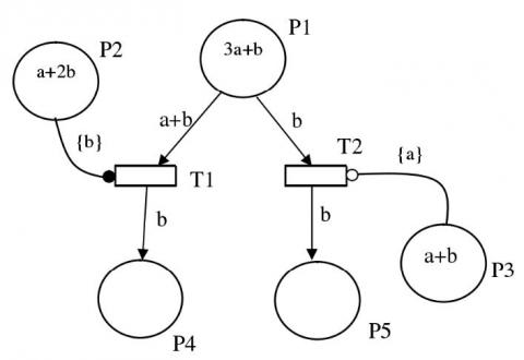
A simple Petri net is described in Figure 1, where each circle stands for a Petri net system, the box represents the transition, the arcs indicate the flow directions, and the solid dots show the symbols in the place.
Figure 1. A simple Petri net
3.2. Extended petri nets
The classic Petri net was modified into new extended Petri nets for the modelling of practical application systems. The modifications are mainly the addition of new elements, making it simpler and more intuitive to describe a particular system. Thus, the extended Petri nets do not outperform the classic Petri net in the descriptive ability of the target system.
The colored Petri net is developed by adding color elements, which mainly classify place and marking, to the classic Petri net. A colored Petri net can be expressed as a seven-tuple $\Sigma=(S, T ; F, C, W, I, M),$ where $(S, T ; F)$ is a net, $C=\left\{c_{1}, c_{2}, \ldots, c_{k}\right\}$ is a finite set of colors, $\mathrm{W} : \mathrm{F} \rightarrow L(C)_{+}, \mathrm{I} : \mathrm{T} \rightarrow L(C)_{+}$ and $\mathrm{M} : \mathrm{S} \rightarrow \mathrm{L}(\mathrm{C}) .$ Note that $\mathrm{L}(\mathrm{C})$ is a linear function of nonnegative integer defined on color set $\mathrm{C}$ and $L(C)_{+}$ refers to the $\mathrm{L}(\mathrm{C})$ whose coefficient is not all zero.
For $\forall t \in T,$ the occurrence condition of transition T under marking $\mathrm{M}$ is $s \in \cdot t \rightarrow$ $M(s) \geq W(s, t) .$ If $\mathrm{M}\left[\mathrm{t}>M^{\prime}, \text { then, the relationship between marking } M^{\prime} \text { and }\right.$ marking $\mathrm{M}$ can be expressed as:
$M^{\prime}(s)=\left\{\begin{array}{c}{M(s)-W(s, t), \quad \text { if } s \in \cdot t-t} \\ {M(s)+W(t, s), \quad \text { if } s \in t^{\cdot}-t} \\ {M(s)-W(s, t)+W(t, s), \quad i f s \in t^{*} \cap \cdot t} \\ {M(s) \text { otherwise }}\end{array}\right.$
The extended Petri net is developed by adding enabling and restraining arcs, which enhance the controllability of the net system, to the classic Petri net. It has been proved that the extended Petri net has a simulation ability equivalent to Turing machine. The enabling and restraining arcs are defined as follows:
(1) Let $F_{I} \sqsubseteq(P \times U)$ be the set of restraining arcs and $F_{E} \sqsubseteq(P \times U)$ be the set of enabling arcs, which satisfy $F_{I} \cap F_{E}=\emptyset$ ;
(2) Let $\mathrm{W} :\left(F_{I} \cup F_{E}\right) \rightarrow\{0\}$ be the weight functions of the two types of arcs.
If $P_{I}$ and $P_{E}$ respectively denote the set of places associated with the enabling and restraining arcs. Then, the transition $t$ can be triggered under marking $\mathrm{M},$ if and only if:
$\left\{\begin{aligned} p \in \cdot t \Rightarrow M(p) \geq W(p, t), p \in\left(P-P_{I}-P_{E}\right) \\ p \in t : M(p)+W(p, t) \leq K(p), p \in P \\ p \in \cdot t \Rightarrow M(p)=0, p \in P_{I} \\ p \in \cdot t \Rightarrow M(p)>0, p \in P_{E} \end{aligned}\right.$
If $\mathrm{M}\left[\mathrm{t}>, \text { then transition t can be triggered under } \mathrm{M}\left[\mathrm{t}>M^{\prime} . \text { In this case, } M^{\prime} \mathrm{can}\right.\right.$ be defined as
$M^{\prime}(p)=\left\{\begin{array}{c}{M(p)-W(p, t), p \in \cdot t-t^{*} \wedge p \in\left(P-P_{I}-P_{E}\right)} \\ {M(p)+W(p, t), p \in t^{*}-t} \\ {M(p)-W(p, t)+W(t, p), p \in t^{*} \cap \cdot t} \\ {M(p) \text { otherwise }}\end{array}\right.$
The extended colored Petri net is a combination of the colored Petri net and the extended Petri net. This net can be developed by adding color elements as well as restraining and enabling arcs into the classic Petri net. The color elements enhance the data description ability, while the two types of arcs control the transition order and depict the event priorities. An extended colored Petri net is a ten-tuple $\Sigma=$ $\left(\mathrm{P}, \mathrm{T} ; \mathrm{F}, \mathrm{C}, W_{F}, I, W_{I}, E, W_{E}, M\right),$ where $\mathrm{P}$ is the set of places, T is the set of transitions,
$\mathrm{C}=\left\{c_{1}, c_{2}, \ldots c_{k}\right\}$ is a finite set of colors, $\mathrm{F} \sqsubseteq(\mathrm{P} \times \mathrm{T}) \cup(\mathrm{T} \times \mathrm{P})$ is a set of finite arcs, $W_{F} : F \rightarrow L(C)_{+}$ is the mapping from finite arc set $\mathrm{F}$ to the color domain, I $\mathrm{L}$ $\mathrm{P} \times$ Tand $\mathrm{E} \sqsubset \mathrm{P} \times \mathrm{T}$ are restraining arc set and enabling arc set, respectively; $\mathrm{M} : \mathrm{P} \rightarrow$ $L(C)$ is the current marking of $\Sigma .$
Figure 2. A simple extended colored petri net
An extended colored petri net can be represented as a directed and weighted bipartite graph, which includes such elements as places, transitions, arcs. The arcs are further divided into restraining/enabling arcs and directed arcs. For the arcs from the place to the transition, those with a small hollow circle are restraining arcs and those with a small solid circle are enabling arcs. As shown in Figure 2, the places are illustrated as circles, the transitions are presented as rectangles, the weight on each directed arc is described as a linear expression of the color set. Different objects or data in a place can be assigned different colors, while different transitions represent different triggering modes.
4.1. Definition of real-time colored petri net
A real-time colored petri net can be expressed as a fourteen-tuple:
$\left(\Sigma, \mathrm{P}, \mathrm{T}, \mathrm{A}, \mathrm{N}, \mathrm{C}, \mathrm{G}, \mathrm{E}, \mathrm{I}, \mathrm{TD},\left[d^{-}, d^{+}\right], T S, P W, S\right)$
where $\Sigma, \quad \mathrm{P}, \mathrm{T}$ and $\mathrm{A}$ are non-empty sets of colors, places, transitions and arcs, respectively, that satisfy $\mathrm{P} \cap \mathrm{T}=\mathrm{P} \cap \mathrm{A}=\mathrm{T} \cap \mathrm{A}=\emptyset ; \mathrm{N}$ is the node function about mapping from $\mathrm{A}$ to $\mathrm{P} \times \mathrm{T}$ LI $\mathrm{T} \times \mathrm{P} ; \mathrm{C}$ is the color function about the mapping from $\mathrm{P}$ to $\Sigma ; \mathrm{G}$ is the guard function about the mapping from $\mathrm{T}$ to expression $\forall \mathrm{t} \in$ $\mathrm{T} :[\text { Type }(\mathrm{G}(\mathrm{t}))=\mathrm{B} \wedge \text { Type }(\mathrm{Var}(\mathrm{G}(\mathrm{t}))) \sqsubseteq \Sigma] ; \mathrm{E}$ is the directed arc expression about $\forall \mathrm{a} \in \mathrm{A} :\left[\text { Type }(\mathrm{E}(\mathrm{a}))=C(p)_{M S} \wedge \mathrm{T} \text { ype }(\operatorname{Var}(\mathrm{E}(\mathrm{a}))) \sqsubseteq \Sigma\right] ;$ I is the initialization function about the mapping from $\mathrm{P}$ to expression $\forall \mathrm{p} \in \mathrm{P} :\left[\text { Type }(\mathrm{I}(\mathrm{p}))=C(p)_{M S}\right]$ TD is a set of random delays between transition enabling and triggering that satisfies $\mathrm{TD}=\mathrm{W}\left(M_{k}\right)$ with $\mathrm{W}\left(M_{k}\right)$ being a distribution function with a certain probability; $\left[d^{-}, d^{+}\right]$ is the allowable trigger interval set for transitions, with $d^{-}$ and $d^{+}$ being the earliest and latest moments allowable to trigger transition, respectively; $T S$ is the timestamp set of marking; $P W : P W \rightarrow R^{[0,1]}$ is the probability of possible transitions that satisfies the expression $\forall p w \in P W : \sum_{t \in p} p w(t)=1 .$ Note that the time information of marking's transit through the place and the transition is contained in $\forall t s \in$ TS. The marking's timestamp information can be calculated by TS = $\sum_{i} t, b_{j} \in Y D(p, t)<b>+\sum_{(t, b) \in Y} D(t, p)<b>+\sum_{t d \in T D} t d .$
Definition 1: The binding of transition $t$ is a function $b$ defined on $\operatorname{Var}(\mathrm{t}),$ which satisfies $\forall \mathrm{v} \in \operatorname{Var}(\mathrm{t}) : \mathrm{b}(\mathrm{v}) \in$ Type $(\mathrm{v}) .$ The set of all bindings is denoted as $\mathrm{B}(\mathrm{t})$
Definition 2: Marking element is defined as (p, c), where p $\in \mathrm{P}$ and $\mathrm{c} \in \mathrm{C}(\mathrm{p})$ Binding element is defined as $(\mathrm{t}, \mathrm{b}),$ where $\mathrm{t} \in \mathrm{T}$ and $\mathrm{b} \in \mathrm{B}(\mathrm{t}) .$ All sets of marking elements are represented by TE, while all sets of binding elements are represented by, while all sets of binding elements are represented by BE. Marking is a multiple set on TE, while step is a non-empty finite multiple set on BE. The initial marking $M_{0}$ is obtained by calculating the initial expression $\forall(p, c) \in$ $\mathrm{TE} : M_{0}(p, c)=(I(p))(c) .$ The sets of markings and steps is denoted as $\mathrm{M}$ and $\mathrm{Y}$ , respectively.
Definition 3: For a marking M, if and only if expression $\forall p \in P : \sum_{(t, b) \in Y} E(p, t)<$ $b>\leq M(p)$ is satisfied, step is considered as enabled. In this case, $(t, b)$ or $t$ is considered as in the enabling state.
Definition $4 :$ When step is enabled under marking $M_{1}$ , the result of the new marking $M_{2}$ can be calculated by $\forall p \in P : M_{2}(p)=M_{1}(p)-\sum_{(t, b) \in Y} E(p, t)<b>$ $+\sum_{(t, b) \in Y} E(t, p)<b>.$ In this case, the marking $M_{2}$ is directly accessible from $M_{1}$ .
Definition 5: A finite occurrence sequence means a sequence of markings and steps satisfying condition $M_{1}\left[Y_{1}>M_{2}\left[Y_{2}>M_{3} \ldots M_{n}\left[Y_{n}>M_{n+1}, \text { where } n \in N, M_{1}\right.\right.\right.$ is the initial marking and $M_{n+1}$ is the new marking.
Definition 6: Marking $M_{j}$ is accessible from marking $M_{i}$ if and only if there is a finite occurrence sequence with $M_{i}$ as the initial marking and $M_{j}$ as the new marking. A marking accessible from $M_{i}$ is denoted as $\left[M_{i}>. \text { Marking } M_{k} \text { is considered as }\right.$ accessible if it satisfies $M_{k} \in\left[\left[M_{0}>. .\right.\right.$
Definition $7 :$ The set of input places of transition $t$ is denoted as $\cdot$ t, which satisfies the expression $\forall p_{i} \in \cdot \mathrm{t} :\left[p_{i} \times t \neq \emptyset, \text { while the set of output places of transition t is }\right.$ denoted as $\mathrm{t} \cdot,$ which satisfies the expression $\forall p_{i} \in \mathrm{t} : :\left[t \times p_{i} \neq \emptyset .\right.$
4.2. Modeling method and analysis
In the hardware design of embedded real-time system, the circuit structure may vary with the design requirements. Based on the real-time colored Petri net, the hardware circuit system is modelled through the following steps:
(1) Each storage unit is represented by a place $p_{i},$ whose data structure definitions are represented by color sets.
(2) Each functional unit is represented by a transition $t_{i},$ the node function $\mathrm{N}\left(t_{i}\right)$ is defined based on the component function, the guard function $\mathrm{G}\left(t_{i}\right)$ is defined according to pre-condition of component function, the allowable trigger interval set for transitions $\left[d^{-}, d^{+}\right]$ and random delay function TD are defined based on the unit's time attribute.
(3) If a functional unit retrieves data from a storage unit, a directed arc will be set up from the corresponding place to the transition.
(4) If the calculation results of the functional unit are imported to the storage unit, a directed arc will be set up from the corresponding transition to the place.
(5) If multiple functional units, with mutually exclusive operations, acquire data from storage units and the operations of these functional units are mutually exclusive, a directed arc expression which is output by the corresponding place of storage units will be set up to describe the probability of transition pw.
(6) The place is initialized according to the actual situation after the circuit system is powered on and reset. Then, the marking elements will be assigned to the corresponding database with data in the storage units, and the marking’s timestamp ts will be defined.
A key function of real-time colored Petri net is the real-time analysis of system performance, which hinges on the worst-case critical path cycle. In a real-time colored Petri net, the critical path consists of a transition sequence $M_{1}\left[Y_{1}>M_{2}\left[Y_{2}>\right.\right.$ $M_{3} \cdots M_{n}\left[Y_{n}>M_{n+1} . \text { The path cycle is actually the time to return to the initial }\right.$ marking $M_{0}$ after at least one transition in the sequence from $M_{0} .$ The minimum path cycle of the system can be expressed as:
$T_{\min }=\max \left\{T_{k} / N_{k} : k=1,2, \ldots, q\right\}$
where $T_{k}$ is the total transition delay in path (circuit) $k ; N_{k}$ is the total number of markings of transition in path (circuit) $k .$
The critical path in the real-time system is the path $k$ that achieves $T_{\min }$
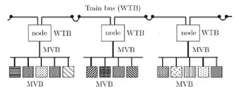
while completing a series of operation cycles. After analyzing the timing information of the critical path, it is possible to optimize the overall performance of the circuit by properly reducing the transition delay or increasing the marking number of the places in the path. In the design phase, the analysis on the time parameters of circuit design is fundamental to the optimization of real-time system performance.Figure 3. Topology of train communication network
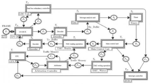
A train communication network (Figure 3) was adopted to verify the effectiveness of our real-time colored Petri net modeling method. As shown in Figure 3, the network has two types of buses, namely, the WTB (wire-train bus) and the MVB (multi-function vehicle bus). The former is responsible for the communication between the boxes, while the latter also supports the communication between devices inside the box. Both types of buses follow the master-slave communication protocol, and have high real-time requirements for data transmission and equipment management. According to real-time colored Petri net modeling method, the author constructed a real-time colored Petri net for MVB bus controller (Figure 4).
Figure 4. Real-time colored petri net for MVB bus controller
Table 1 lists the worst-case time parameters of each functional unit to complete the operation.
Table 1. Worst-case operation time of functional units
|
Transition sequence number |
Functional unit |
Longest delay (ns) |
|
T1 |
Decoder |
3160 |
|
T2 |
Message analysis unit |
30 |
|
T3 |
Timer |
3 |
|
T4 |
Main control unit |
6 |
|
T5 |
Traffic message channel (TMC) reading operation |
20 |
|
T6 |
Encoder |
30 |
|
T7 |
CPU |
280 |
|
T8 |
Arbitrator |
20 |
|
T9 |
TMC writing operation |
20 |
|
T10 |
Interrupt controller |
400 |
|
T11 |
Dual bus redundancy controller |
15 |
|
T12 |
Input/output multiplexer (I/O MUX) |
30 |
The T_reply is an important parameter that must be configured by the MVB bus controller at the start of train operation. Here, it is cited as an example to illustrate how system time parameters are determined by real-time colored Petri net analysis. The T_reply refers to the maximum delay from the transmitting end to the receiving end of the main frame monitored by the main control unit. The value of this parameter equals the sum of data transmission time, decoding time and access time:
T_ reply $=2 \times\left(6.0 \times L+T_{\text {repeat }} \max \times \text { Nrep }\right)+T_{-}$ source_ $\max$
where 6.0$\mu \mathrm{s} / \mathrm{km}$ is worst-case delay of bus transmission; $L$ is the length of the line; $T_{-}$ repeat $\max$ is the maximum delay caused by repeaters; Nrep is the number of repeaters; $T_{-}$ source. $\max$ is maximum delay at the end of the data source.
Next, all s-invariants, which represent the paths in the circuit, were obtained from the incidence matrix of real-time colored Petri net. Table 2 shows the s-invariants, as well as the corresponding paths and delays.
Table 2. s-invariants and corresponding paths and delays
|
s-invariant |
Paths |
Delay (ns) |
|
Y1 |
T1 T2 T3 T4 T5 T6 T12 |
3,379 |
|
Y2 |
T11 T12 |
45 |
|
Y3 |
T1 T2 T4 T9 T8 T5 T6 T12 |
3,316 |
|
Y4 |
T1 T2 T4 T10 T7 T8 T5 T6 T12 |
3,976 |
|
Y5 |
T11 T10 T7 T8 T5 T6 T12 |
795 |
|
Y6 |
T12 |
30 |
|
Y7 |
T7 T8 |
300 |
|
Y8 |
T1 T2 T4 T5 T6 T12 |
3,376 |
It can be seen from Table 2 that the critical paths of MVB bus controller are T1 T2 T4 T10 T7 T8 T5 T6 T12. The path delay peaked at 3,976ns. The time parameters obtained are in line with the real-time requirements on T_source in the Train Communication Network IEC 61375. This means the designed MVB bus controller fulfils the strict real-time requirements of the train system and benefits the real-time performance of the whole train system.
This paper probes into the modeling and analysis methods of embedded real-time systems, and extends the colored Petri net into a real-time colored Petri net model. The proposed model was applied to simulate the MVB bus controller of train communication network. Through real-time analysis of the simulation results, it is proved that the proposed embedded real-time system modelling approach can fulfil the strict real-time requirements of the train system. The research findings shed new light on the application of Petri nets and the simulation of embedded real-time systems.
Hubei Provincial Department of Education Scientific Research Project B2016087. Shiyan South-to-North Water Transfer Counterpart Collaborative Project 2017syn043A.
Berthomieu B., Diaz M. (1991). Modeling and verification of time dependent systems using time petri nets. IEEE Trans on Software Eng, Vol. 17, No. 3, pp. 259-273. https://doi.org/10.1109/32.75415
Chen H., Amodeo L., Chu F., Labadi K. (2005). Modeling and performance evaluation of supply chains using batch deterministic and stochastic petri nets. IEEE Transactions on Automation Science and Engineering, Vol. 2, No. 2, pp. 144. https://doi.org/10.1109/TASE.2005.844537
Chen R., Sgroi M., Lavagno L., Martin G., Sangiovanni-Vincentelli A., Rabaey J. (2001). Embedded system design using UML and platforms. System Specification & Design Languages, pp. 119-128. https://doi.org/10.1007/0-306-48734-9_10
Gardey G., Roux O. H., Roux O. F. (2005). State space computation and analysis of time petri nets. Theory & Practice of Logic Programming, Vol. 6, No. 3, pp. 301-320. https://doi.org/10.1017/S147106840600264X
Hsiung P. A., Gau C. H. (2002). Formal synthesis of real-time embedded software by time-memory scheduling of colored time petri nets 1. Electronic Notes in Theoretical Computer Science, Vol. 65, No. 6, pp. 140-159. https://doi.org/10.1016/S1571-0661(04)80474-2
Huang C. C., Liang W. Y. (2004). Object-oriented development of the embedded system based on petri-nets. Computer Standards & Interfaces, Vol. 26, No. 3, pp. 187-203. https://doi.org/10.1016/j.csi.2003.08.001
Jensen K., Kristensen L. M., Wells L. (2007). Coloured petri nets and CPN tools for modelling and validation of concurrent systems. International Journal on Software Tools for Technology Transfer, Vol. 9, No. 3-4, pp. 213-254. https://doi.org/10.1007/s10009-007-0038-x
Jiang C., Ataai M., Ozuer A., Krisky D., Wechuck J., Pornsuwan S. (2000). Formal verification of real-time system requirements. Computer Science, Vol. 2, No. 1, pp. 813-819. https://doi.org/10.1016/j.jhazmat.2009.02.096
Kaakai F., Hayat S., Moudni A. E. (2007). A hybrid petri nets-based simulation model for evaluating the design of railway transit stations. Simulation Modelling Practice & Theory, Vol. 15, No. 8, pp. 935-969. https://doi.org/10.1016/j.simpat.2007.05.003
Liu D., Wang J., Chan S. C. F., Sun J., Zhang L. (2002). Modeling workflow processes with colored petri nets. Computers in Industry, Vol. 49, No. 3, pp. 267-281. https://doi.org/10.1016/s0166-3615(02)00099-4
Maciel P., Barros E., Rosenstiel W. (1999). A petri net model for hardware/software codesign. Design Automation for Embedded Systems, Vol. 4, No. 4, pp. 243-310. https://doi.org/10.1023/a:1008969621405
Peterson J. L. (2010). Petri net theory and the modeling of systems. Computer Journal, Vol. 25, No. 1. https://doi.org/ 10.1093/comjnl/25.1.129
Rettberg J. A. (2015). A program state machine based virtual processing model in systemc. Acm Sigbed Review, Vol. 11, No. 4, pp. 7-12. https://doi.org/10.1145/2724942.2724943
Zuberek W. M. (1991). Timed petri nets definitions, properties, and applications. Microelectronics Reliability, Vol. 31, No. 4, pp. 627-644. https://doi.org/10.1016/0026-2714(91)90007-T