
Mohammed Ali Alfayizi
© 2026 The author. This article is published by IIETA and is licensed under the CC BY 4.0 license (http://creativecommons.org/licenses/by/4.0/).
OPEN ACCESS
Velocity-direction-based adaptive super-twisting sliding-mode control (ASTSMC) is investigated for a steering-rate-controlled car-like mobile robot during disturbed cornering. Five paired MATLAB scenarios compare the proposed controller with an adaptive heading-feedback baseline using unchanged tuning. The nominal case has a 2.50 m turn radius, 0.65 m/s reference speed, 32 s horizon, and sinusoidal motion-direction perturbation of amplitude 0.42 rad/s over 8–24 s. Additional cases vary curvature, speed, disturbance amplitude, and initial tracking error separately. In the nominal case, planar, lateral, and velocity-direction root-mean-square errors decrease by 68.67%, 86.88%, and 92.87%, respectively, while integrated steering-rate effort decreases by 17.86%. Additional-case planar-error reductions range from 50.01% to 94.94%, with lower integrated steering-rate effort in every pair. Trajectory, error, steering, and gain histories identify both disturbance response and subsequent recovery. The analytical steering-rate formulations are distinguished from the evaluated heading-feedback baseline and motion-direction disturbance channel. The results support improved tracking for the implemented controllers and tested conditions, without establishing physical-robot accuracy or universal superiority.
adaptive super-twisting sliding-mode control, car-like mobile robot, geometric slip angle, kinematic bicycle model, steering-rate disturbance, velocity direction
Car-like mobile robots combine nonholonomic rolling constraints with steering and longitudinal actuation. Applications include campus transportation, inspection platforms, service robots, and low-speed automated mobility. Classical work establishes the kinematic classification and feedback-control problem [1, 2], while planning studies explain the associated non-integrable constraints and turning restrictions [3, 4]. Automated-driving surveys connect these requirements to feasible motion planning and control [5]. Recent car-like robot studies also address tracking under slipping and skidding and observer-based disturbance compensation [6, 7].
The present study investigates the steering objective used to track the center of a car-like robot during disturbed cornering. It complements robust vehicle trajectory-following research [8] by examining trajectory deviation, recovery, and steering-command demand with a fixed controller configuration. For an automated robot system, the relevant benefit is accurate motion with the available steering authority, rather than angular alignment considered independently of the position response.
Body heading or yaw $\psi$ is a natural steering variable because it describes chassis orientation and appears in bicycle-model dynamics [9, 10]. Geometric path-following methods use heading and path-tangent information [11, 12], while robust and sliding-mode studies regulate orientation-related errors [13, 14]. A controller that assigns the center-path direction directly as the heading reference can retain a geometric directional offset in a turn; this does not imply that all heading-based methods lack compensation.
For a car-like robot modeled at the geometric center, however, the translational velocity of the center is not generally aligned with the body heading. In the center-based kinematic bicycle model, the position evolves according to the effective velocity-direction angle
$\theta_v=\psi+\beta$ (1)
where $\beta$ is the steering-induced geometric offset determined by steering angle and axle geometry. Consistent bicycle and predictive-control models account for the distinction between body heading and center velocity direction [15, 16]. Predictive steering and driving-envelope studies also incorporate yaw, sideslip, and feasibility considerations [17-19]. The physical quantity $\theta_v$ is therefore established; the present control question is how direct regulation of this quantity behaves in the selected low-speed, steering-rate-controlled formulation.
Sliding mode control (SMC) provides a framework for matched-uncertainty rejection [20-23]. Standard and higher-order sliding-mode concepts are summarized in the study [24], with sliding order, accuracy, and output-feedback developments in studies [25, 26]. The super-twisting algorithm combines a continuous ideal control action with discontinuous auxiliary dynamics; strict Lyapunov constructions establish convergence under suitable perturbation and gain conditions [27]. These conditions must be distinguished from finite-horizon behavior with saturation and sampled implementation.
Adaptive sliding mode control and adaptive super-twisting structures address dependence on conservative fixed gains [28-30]. These methods motivate the proposed adaptive super-twisting sliding-mode control (ASTSMC), while their sufficient conditions remain distinct from the numerical implementation choices described in Section 6.1. Related robot and vehicle studies investigate adaptive feedback, disturbance observers, neural compensation, and generalized super-twisting laws for trajectory tracking [31-39].
Recent work provides useful distinctions. Sun et al. [40] combine fixed-time generalized super-twisting control with wheel-slip compensation for agricultural path tracking and report simulation and field validation. Their physical slip treatment differs from the geometric offset and deterministic motion-direction benchmark used here. He et al. [41] compare body-yaw and travel-direction descriptions in a Takagi–Sugeno fuzzy tracking model, with simulation and hardware-in-the-loop validation. Their term “heading angle” denotes travel direction, whereas $\psi$ denotes body heading in this paper. Their steering-angle-input model and fuzzy robust-control realization differ from the present steering-rate command and adaptive super-twisting structure. Sun and Zhu [42] combine model predictive and sliding mode control in a dual-model lateral path-tracking controller. Maaruf and Mysorewala [43] address external disturbances and input dead zones through neural backstepping, command filtering, and simulation. Hosseinnajad et al. [44] develop a double-surface homogeneous sliding-mode approach with actuator limitations for self-driving lateral control. These studies motivate explicit reporting of the controlled quantity, uncertainty channel, and actuator assumptions rather than a blanket claim that prior heading-based methods omit slip or constraints.
These studies address different combinations of output selection, slip compensation, uncertainty estimation, and actuator constraints. The specific question here is the behavior of a velocity-direction-based adaptive super-twisting controller relative to an adaptive heading-feedback baseline during center-trajectory cornering and recovery. Table 1 compares that scope with recent work. The distinction is the combination of the regulated center-motion direction, direct steering-rate command, and fixed-tuning S0–S4 evaluation; it is not a claim that velocity direction or slip compensation was previously absent from vehicle control.
Table 1. Related control approaches and the scope of the present comparison
|
Study |
Regulated Quantity/Model |
Robustness or Constraint Treatment |
Validation Reported |
Distinction from S0–S4 |
|
Sun et al. [40] |
Agricultural vehicle path tracking with wheel slipping |
Fixed-time generalized super-twisting and slip compensation |
Simulation and field tests |
Physical wheel-slip treatment, not the present motion-direction benchmark |
|
He et al. [41] |
Body-yaw versus travel-direction vehicle models |
Takagi–Sugeno fuzzy robust control; steering angle input |
Simulation and hardware-in-the-loop tests |
Directly treats output choice, but with a different plant and control realization |
|
Sun and Zhu [42] |
Autonomous-vehicle lateral path tracking |
Model predictive/sliding mode dual-model controller |
MATLAB/CarSim co-simulation |
Different feedback architecture; not the retained adaptive heading baseline |
|
Maaruf and Mysorewala [43] |
Ground-vehicle path following |
Neural backstepping, command filtering, input-deadzone compensation |
Simulation |
Actuator dead zone is distinct from the adaptation dead zones used here |
|
Hosseinnajad et al. [44] |
Self-driving lateral control |
Double-surface homogeneous sliding mode; actuator limitations |
Simulation |
Dynamic lateral-control setting, rather than this fixed-tuning kinematic benchmark |
|
Present study |
Center-velocity direction versus an implemented heading-feedback baseline |
Adaptive super-twisting rate command, fixed angle/rate bounds, interval perturbation |
Five paired MATLAB scenarios |
Unchanged tuning across curvature, speed, disturbance, and initial-error variations |
Note: The table compares problem formulations and validation scope; it is not a performance ranking across different datasets.
The numerical evidence consists of five paired scenarios, S0–S4, using the same controller functions and tuning throughout. S0 retains the original comparison, while S1–S4 vary curvature, speed, disturbance amplitude, and initial error individually. Section 4.2 also retains an analytical heading-based super-twisting reference formulation to explain the different input–output pathways; that formulation is not the adaptive heading-feedback baseline used to generate S0–S4. Sections 4.4 and 6.1 identify the scope of each formulation so that the numerical comparison is attributed to the controllers actually evaluated.
The main contributions of this work are summarized as follows:
•A center-based nonlinear kinematic formulation explains why the body heading $\psi$ and effective velocity direction $\theta_v=\psi+\beta$ have different roles during cornering.
•The control design separates nominal heading dynamics from the geometric steering contribution to the center-velocity-direction channel.
•A velocity-direction-based ASTSMC formulation regulates the angular variable governing center translation through a direct steering-rate command.
•Ideal-regime boundedness and sliding-convergence arguments are stated with their assumptions and separated from the finite-horizon evidence under sampling and saturation.
•Five paired scenarios evaluate tracking, post-disturbance recovery, steering input, and adaptive gains with unchanged tuning, including the stronger-disturbance case in which the baseline loses accurate tracking.
Section 2 presents the center-based model and its physical interpretation. Section 3 defines the tracking objectives and analytical disturbance assumptions. Section 4 presents the controller formulations and distinguishes them from the implemented comparison. Section 5 discusses conditional stability and practical limitations. Section 6 reports the S0–S4 settings and results, followed by engineering interpretation in Section 7 and conclusions in Section 8.
2.1 Robot description
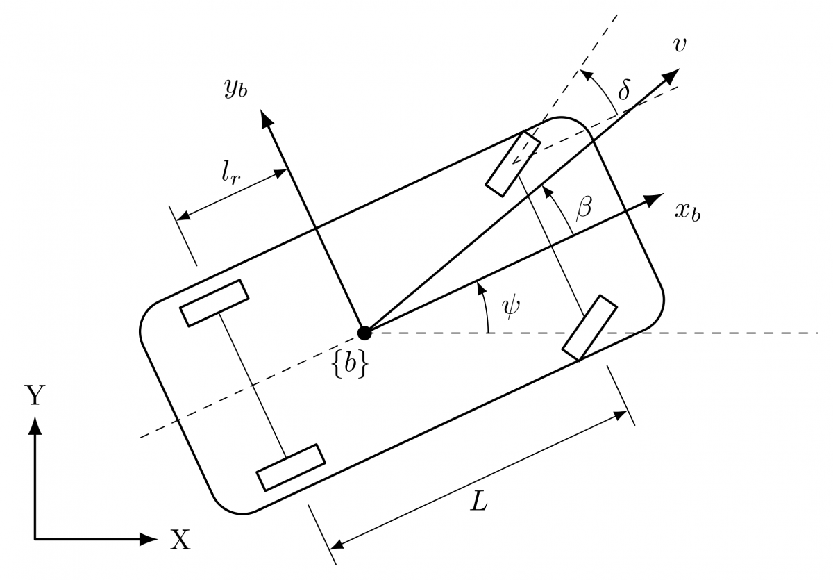
A car-like mobile robot operating on a planar surface is considered (Figure 1). The posture of the robot is defined by the Cartesian coordinates of its geometric center, (x, y), alongside the body heading angle, $\psi$. Furthermore, the longitudinal speed and the steering angle are denoted by $v$ and $\delta$, respectively. The vehicle wheelbase is specified as $L$, while the longitudinal distance from the geometric center to the rear axle is represented by $l_r$.
Figure 1. Schematic diagram of the car-like mobile robot with the coordinate frame located at the geometric center. The two front wheels are shown with the same positive steering angle $\delta$
In Figure 1, $X, Y$ are inertial axes and $x_b, y_b$ are body-fixed axes at the selected center point {b}. The angle $\psi$ is measured from $X$ to $x_b, \delta$ is the equivalent front-wheel steering angle, $L$ is wheelbase, and $l_r$ is the rear-axle-to-center distance. The speed $v$ is the center-velocity magnitude; its body-longitudinal component is $v \cos \beta$. The angle $\beta$ describes the offset of that velocity from the chassis axis, not a separate tire-deformation sideslip state. The equal front-wheel angles in the schematic are a bicycle-model representation, not the unequal wheel angles of a finite-track-width Ackermann linkage. Center-based coordinates are appropriate because the desired trajectory and reported position errors refer to that point; a rear-axle representation is appropriate when the rear axle is the tracking point.
The reference speeds are 0.65–0.70 m/s. On the prescribed constant-speed arcs, the kinematic reference quantity $v_d{ }^2 / R_c$ ranges from approximately 0.141 to 0.196 m/s² across S0–S4. These operating values describe the test trajectory, not a validated tire-friction or vehicle-stability boundary. Tire parameters are absent, so the low-speed simplification should not be extrapolated to dynamic sideslip, high-speed lane changes, or a specified physical vehicle without further validation [9, 15].
2.2 Center-based kinematic bicycle model
The nominal low-speed geometry is represented by a kinematic bicycle model. The center velocity forms an angle $\beta$ with the body-longitudinal axis, with [16]
$\beta=\tan ^{-1}\left(\frac{l_r}{L} \tan \delta\right)$ (2)
The corresponding nominal kinematic relations are [15, 16]
$\dot{x}=v \cos (\psi+\beta)$ (3)
$\dot{y}=v \sin (\psi+\beta)$ (4)
$\dot{\psi}=\frac{v}{L} \tan (\delta) \cos (\beta)$ (5)
The longitudinal speed and steering-angle dynamics are described by
$\dot{v}=a$ (6)
$\dot{\delta}=\omega_\delta$ (7)
where $a$ is the longitudinal acceleration and $\omega_\delta$ is the steering-rate input.
Therefore, the complete state vector of the system can be expressed as
$\mathrm{q}=\left[\begin{array}{lllll}x & y & \psi & v & \delta\end{array}\right]^T$ (8)
3.1 Control objective
The objective of this study is to design the control inputs
$\mathrm{u}(t)=\left[a(t) \quad \omega_\delta(t)\right]^T$ (9)
such that center-position and direction errors are reduced while the applied steering commands respect their prescribed limits. The design objective is accurate tracking and recovery in the presence of bounded perturbations. Conditional ideal-regime analysis and the finite-horizon constrained simulations provide different types of evidence and are interpreted separately.
3.2 Reference trajectory and tracking errors
Let the desired trajectory be described by the reference pose
$\mathrm{q}_d=\left[\begin{array}{lll}x_d & y_d & \psi_d\end{array}\right]^T$ (10)
The trajectory-tracking errors are defined within the robot body-fixed frame as
$\left[\begin{array}{l}e_x \\ e_y \\ e_\psi\end{array}\right]=\left[\begin{array}{ccc}\cos \psi & \sin \psi & 0 \\ -\sin \psi & \cos \psi & 0 \\ 0 & 0 & 1\end{array}\right]\left[\begin{array}{l}x_d-x \\ y_d-y \\ \psi_d-\psi\end{array}\right]$ (11)
Here, $e_x$ and $e_y$ denote the longitudinal and lateral position errors expressed in the body-fixed frame, while $e_\psi$ denotes the heading-angle error. Through this body-frame representation, the position error is decomposed into along-track and crosstrack components relative to the robot orientation. In particular, the lateral error $e_y$ is utilized within the steering-control design to quantify the deviation of the geometric center from the desired path.
3.3 Geometric slip angle and effective motion direction
Within the adopted center-based kinematic bicycle model, the translational motion of the geometric center is governed by Eqs. (3)–(4), wherein the steering-induced geometric slip angle $\beta$ is defined by Eq. (2).
In this formulation, $\beta$ characterizes the geometric offset between the body heading angle and the true velocity direction of the geometric center. Consequently, the effective velocity-direction angle is established in Eq. (1).
These relationships demonstrate that the translational trajectory of the geometric center is dictated by the effective velocity-direction angle $\theta_\nu$, rather than by the body heading angle $\psi$ alone. Consequently, $\theta_v$ is proposed as the primary steering variable for the advanced tracking controller. By adopting this formulation, the steering-induced geometric offset $\beta$ is directly incorporated into the regulated motion direction, a feature that is particularly critical during cornering maneuvers.
3.4 Compared steering variables
The analytical discussion compares heading and velocity-direction steering objectives within the same nominal kinematic geometry. In the heading formulation, the angular error is $e_\psi$ in Eq. (11). For the proposed formulation, $\theta_{v, d}$ denotes the desired center-velocity direction associated with the guidance law. Its error is
$e_{\theta_v}=\theta_{v, d}-\theta_v$ (12)
The heading objective concerns body orientation, whereas the proposed objective concerns the center-velocity direction. The desired tracking behavior is small planar error together with the relevant angular error, summarized as
$e_x(t) \rightarrow 0, \quad e_y(t) \rightarrow 0$ (13)
together with either
$e_\psi(t) \rightarrow 0 \quad$ or $\quad e_{\theta_v}(t) \rightarrow 0$ (14)
for the selected formulation. These expressions describe tracking objectives, not an unconditional convergence claim for the saturated numerical implementation.
The numerical comparison evaluates the proposed velocity-direction controller against the implemented adaptive heading-feedback baseline under identical scenario conditions. It does not isolate output choice from controller structure or tuning.
3.5 Disturbance and actuator constraints
For the analytical steering-actuator model, a matched perturbation $d_m(t)$ is introduced into the steering-rate dynamics. On intervals where the regularity assumptions apply, it satisfies
$\left|d_m(t)\right| \leq \bar{d}_m, \quad\left|\dot{d}_m(t)\right| \leq \bar{\rho}_m$ (15)
where $\bar{d}_m>0$ and $\bar{\rho}_m>0$ represent unknown positive constants. Consequently, the perturbed steering dynamics are formulated as
$\dot{\delta}=\omega_\delta+d_m(t)$ (16)
Eq. (16) is the analytical steering-actuator disturbance model used in the derivation of Section 4. It is not the disturbance-injection rule used to generate the S0–S4 benchmark.
The numerical benchmark applies $d_\theta(t)$ directly to the effective motion-direction derivative, as specified in Eqs. (94)–(95), while the steering angle is advanced from the commanded rate and constrained to its admissible interval. The two channel descriptions are not assumed equivalent. The S0–S4 comparisons use the same implemented channel for both controllers, with its parameters held fixed except for the amplitude change in S3.
The steering angle is strictly bounded by the physical actuator constraint
$|\delta(t)| \leq \delta_{\max}$ (17)
while the steering-rate input is constrained such that
$\left|\omega_\delta(t)\right| \leq \omega_{\max}$ (18)
The steering constraints are imposed independently of the desired tracking accuracy. In the ideal analysis, boundedness of the quantities
$v \left( t \right), |\omega_{\delta } \left( t \right), |\beta \left( t \right)$ (19)
is considered under the stated assumptions. In the numerical benchmark, rate clipping and steering-angle projection enforce their respective limits; these mechanisms do not by themselves guarantee convergence of the position errors.
This section presents the common guidance law, an analytical heading-based super-twisting reference formulation, and the proposed velocity-direction-based formulation. The analytical reference explains how heading regulation can be realized through a virtual heading-rate command and inner steering loop. The numerical baseline is instead the adaptive heading-feedback implementation described in Section 6.1. It shares the scenario, geometry, guidance, and actuator limits with the proposed method, but not an identical steering law or gain-adaptation structure.
For the nominal plant, the steering-rate input $\omega_\delta$ affects $\theta_v$ through the derivative of the geometric offset, whereas its effect on $\psi$ is mediated by the steering state $\delta$. This motivates the virtual-rate construction in Section 4.2 and the direct rate command in Section 4.3. Their mathematical comparison is distinguished from the two implemented algorithms evaluated in S0-S4.
4.1 Common guidance law
Let the auxiliary translational guidance signals be defined as
$u_x=\dot{x}_d+k_x\left(x_d-x\right)$ (20)
$u_y=\dot{y}_d+k_y\left(y_d-y\right)$ (21)
where $k_x>0$ and $k_y>0$ are design gains.
The desired translational speed is selected as
$v_c=\sqrt{u_x^2+u_y^2}$ (22)
and the desired path direction is defined by
$\theta_{v, d}=\operatorname{atan} 2\left(u_y, u_x\right)$ (23)
Its time derivative is given by
$\dot{\theta}_{v, d}=\frac{u_x \dot{u}_y-u_y \dot{u}_x}{u_x^2+u_y^2}$ (24)
The common ideal longitudinal law is stated below. The numerical implementation uses the same guidance structure with speed and acceleration limits, as described in Section 6.4. Define the speed-tracking error as
$e_v=v-v_c$ (25)
Then, the longitudinal acceleration input in Eq. (6) is chosen as
$a=\dot{v}_c-k_v e_v$ (26)
where $k_v>0$ is the longitudinal gain.
In the sampled benchmark, the speed command and acceleration are limited and the computed speed derivative is used as implemented. Consequently, the exact unlimited relation in Eq. (26) supplies the ideal design reference, while the constrained numerical speed channel is assessed through the recorded responses.
4.2 Analytical heading-based super-twisting formulation
For the analytical heading-based reference formulation, the desired body heading is assigned from the guidance direction as
$\psi_d=\theta_{v, d}$ (27)
This analytical reference aligns $\psi$ with the guidance direction, whereas the proposed formulation aligns $\theta_v=\psi+\beta$ with that direction. The numerical heading baseline additionally uses the look-ahead correction described in Section 6.1. For the analytical reference, the heading error is
$e_\psi=\psi_d-\psi$ (28)
To establish coupling between the heading error and the lateral body-frame error, the heading-based sliding variable is formulated as
$s_\psi=e_\psi+\lambda_y e_y$ (29)
where $\lambda_y>0$ represents a positive design coefficient.
Because the steering-rate input does not directly affect the heading dynamics, a virtual heading-rate command is utilized. Let
$r_\psi=\dot{\psi}$ (30)
Based on the kinematic model, this is expressed as
$r_\psi=\frac{v}{L} \tan \delta \cos \beta$ (31)
Differentiating Eq. (29) yields
$\dot{s}_\psi=\dot{\psi}_d-r_\psi+\lambda_y \dot{e}_y$ (32)
To achieve an adaptive super-twisting structure [29] within the virtual heading-rate channel, the command $r_{\psi, c}$ is specified as
$r_{\psi, c}=\dot{\psi}_d+\lambda_y \dot{e}_y+k_1^\psi(t)\left|s_\psi\right|^{1 / 2} \operatorname{sgn}\left(s_\psi\right)-z_\psi$ (33)
governed by the auxiliary dynamics
$\dot{z}_\psi=-k_2^\psi(t) \operatorname{sgn}\left(s_\psi\right)$ (34)
Furthermore, the adaptive gains are defined as
$k_1^\psi(t)=k_{1, \min}^\psi+\rho_1^\psi(t)$ (35)
$k_2^\psi(t)=k_{2, \min}^\psi+\rho_2^\psi(t)$ (36)
where $k_{1, \min}^\psi>0$ and $k_{2, \min}^\psi>0$ establish the minimum gain bounds. The corresponding adaptive states satisfy
$\dot{\rho}_1^\psi=\gamma_1^\psi\left|s_\psi\right|-\sigma_1^\psi \rho_1^\psi$ (37)
$\dot{\rho}_2^\psi=\gamma_2^\psi\left|s_\psi\right|-\sigma_2^\psi \rho_2^\psi$ (38)
subject to the initial conditions
$\rho_1^\psi(0) \geq 0, \quad \rho_2^\psi(0) \geq 0$ (39)
with $\gamma_1^\psi, \gamma_2^\psi>0$ designating the adaptation rates and $\sigma_1^\psi, \sigma_2^\psi>0$, representing the leakage coefficients.
A regularized steering-angle conversion is constructed from the nominal heading-rate relation in Eq. (31). It evaluates the geometric factor at the current steering state and is not asserted to be an exact implicit inverse. The steering-angle command is constrained using the saturation operator
$\operatorname{sat}_{\delta_{\max}}(\chi)= \begin{cases}\delta_{\max}, & \chi>\delta_{\max} \\ \chi, & -\delta_{\max} \leq \chi \leq \delta_{\max} \\ -\delta_{\max}, & \chi<-\delta_{\max}\end{cases}$ (40)
Consequently, the commanded steering angle is given by
$\delta_{\psi, c}=\operatorname{sat}_{\delta_{\text {max}}}\left[\tan ^{-1}\left(\frac{L r_{\psi, c}}{v \cos \beta+\varepsilon_v}\right)\right]$ (41)
where $\varepsilon_v>0$ is a small regularization constant employed to mitigate potential singularities when the effective forward velocity component $v \cos \beta$ approaches zero. This term provides numerical stability during low-speed operation while exerting negligible influence during standard motion where $(v \cos \beta)^2 \gg \varepsilon_v^2$.
Because the steering angle constitutes a system state while the actual control input is the steering rate, the heading-based steering law is constructed via an inner loop:
$\omega_\delta=\operatorname{sat}_{\omega_{\max}}\left(k_{\delta, \psi}\left(\delta_{\psi, c}-\delta\right)\right)$, (42)
where $k_{\delta,\psi} > 0$ denotes the inner steering-loop gain.
Eqs. (26), (33), (34), (41), and (42), with Eqs. (37)–(38), define the analytical heading-based super-twisting reference. Its coefficients $k_{1}^{\psi}$ and $k_{2}^{\psi}$ are not the numerical baseline gains $k_{\psi}$ and $k_{\delta}$ plotted in Section 6.
4.3 Adaptive velocity-direction super-twisting control
The proposed controller regulates the effective motion direction $\theta_{v}$, defined in Eq. (1). The corresponding angular tracking error is $e_{\theta_{v}}$, defined in Eq. (12).
The velocity-direction-based sliding variable is chosen as
$s_{\theta_{v}} = e_{\theta_{v}} + \lambda_{y} e_{y}$ (43)
For the analytical disturbance model in Eq. (16), differentiation of the geometric slip angle gives
$\dot{\beta} = G \left( \delta \right) \left( \omega_{\delta} + d_{m} \left( t \right) \right)$ (44)
where
$G \left( \delta \right) = \frac{\frac{l_{r}}{L} \sec^{2} \delta}{1 + \left( \frac{l_{r}}{L} \tan \delta \right)^{2}}$ (45)
Therefore, the effective motion-direction dynamics are
$\dot{\theta}_{v} = \frac{v}{L} \tan \delta \cos \beta + G \left( \delta \right) \left( \omega_{\delta} + d_{m} \left( t \right) \right)$ (46)
Equivalently,
$\dot{\theta}_{v} = \frac{v}{L} \tan \delta \cos \beta + G \left( \delta \right) \omega_{\delta} + \Delta_{m} \left( t \right)$ (47)
where
$\Delta_{m} \left( t \right) = G \left( \delta \right) d_{m} \left( t \right)$ (48)
is the matched perturbation induced in the effective motion-direction channel.
Differentiating Eq. (43) yields
$\dot{s}_{\theta_{v}} = \dot{\theta}_{v,d} - \dot{\theta}_{v} + \lambda_{y} \dot{e}_{y}$ (49)
Substituting Eq. (47) into Eq. (49) gives
$\dot{s}_{\theta_{v}} = \dot{\theta}_{v,d} + \lambda_{y} \dot{e}_{y} - \frac{v}{L} \tan \delta \cos \beta - G \left( \delta \right) \omega_{\delta} - \Delta_{m} \left( t \right)$ (50)
Define the nominal lumped term
$F_{\theta_{v}} = \dot{\theta}_{v,d} + \lambda_{y} \dot{e}_{y} - \frac{v}{L} \tan \delta \cos \beta$ (51)
Then
$\dot{s}_{\theta_{v}} = F_{\theta_{v}} - G \left( \delta \right) \omega_{\delta} - \Delta_{m} \left( t \right)$ (52)
The proposed super-twisting structure gives the unsaturated steering-rate command
$\omega_{\delta}^{\star} = G \left( \delta \right)^{-1} \left( F_{\theta_{v}} + k_{1}^{\theta} \left( t \right) \left| s_{\theta_{v}} \right|^{1/2} \operatorname{sgn} \left( s_{\theta_{v}} \right) - z_{\theta} \right)$ (53)
with the auxiliary dynamics
$\dot{z}_{\theta} = - k_{2}^{\theta} \left( t \right) \operatorname{sgn} \left( s_{\theta_{v}} \right)$ (54)
The adaptive gains are defined as
$k_{1}^{\theta} \left( t \right) = k_{1,\min}^{\theta} + \rho_{1}^{\theta} \left( t \right)$ (55)
$k_{2}^{\theta} \left( t \right) = k_{2,\min}^{\theta} + \rho_{2}^{\theta} \left( t \right)$ (56)
and the adaptive states satisfy
$\dot{\rho}_{1}^{\theta} = \gamma_{1}^{\theta} \left| s_{\theta_{v}} \right| - \sigma_{1}^{\theta} \rho_{1}^{\theta}$ (57)
$\dot{\rho}_{2}^{\theta} = \gamma_{2}^{\theta} \left| s_{\theta_{v}} \right| - \sigma_{2}^{\theta} \rho_{2}^{\theta}$ (58)
with
$\rho_{1}^{\theta} \left( 0 \right) \geq 0, \rho_{2}^{\theta} \left( 0 \right) \geq 0$ (59)
To preserve physical feasibility, the applied steering-rate input is saturated as
$\omega_{\delta} = \mathrm{sat}_{\omega_{\max}} \left( \omega_{\delta}^{\star} \right)$ (60)
Eqs. (26), (53), (54), and (60), with the sliding variable in Eq. (43), the term in Eq. (51), and Eqs. (57)–(58), specify the ideal velocity-direction formulation. The evaluated sampled implementation uses the same super-twisting command structure, a backward-difference lateral-error derivative, and the adaptation dead zone specified in Section 6.1.
4.4 Scope of the analytical and numerical comparisons
The analytical formulations share the ideal longitudinal law and super-twisting structure, while their different relative degrees require different steering realizations. Their regulated angular errors are
$\begin{array}{c}\text{heading-based controller:} \,\,e_{\psi}, \\ \text{velocity-direction-based controller:} \,\,e_{\theta_{v}}\end{array}$ (61)
The numerical question is more specific: under the common S0–S4 test conditions, how does the implemented velocity-direction controller compare with the adaptive heading-feedback baseline in center tracking, recovery, and steering-command demand?
Identical scenario conditions and unchanged tuning make the paired tests reproducible, but do not establish that all differences result from the angular variable alone. The numerical baseline, its look-ahead reference, and the motion-direction disturbance channel are stated in Section 6.1. Consequently, Theorem 1 describes the analytical reference of Section 4.2, not the simulated heading baseline; the S0–S4 results are not presented as an experimental verification of that theorem.
The following analysis concerns the ideal analytical formulations of Section 4. Conditional gain boundedness and ideal sliding convergence are discussed under the assumptions below. The heading formulation additionally requires a sufficiently regular inner-loop residual. Section 5.5 explains its relationship to sampled, constrained operation.
Assumption 1. The reference trajectory is assumed to be sufficiently smooth, such that the signals $x_{d}$, $y_{d}$, $\dot{x}_{d}$, $\dot{y}_{d}$, $\ddot{x}_{d}$, and $\ddot{y}_{d}$ are uniformly bounded.
Assumption 2. The guidance signals generated via Eqs. (20)-(24) are assumed to satisfy
$\left| v_{c} \left( t \right) \right| \leq \overline{v}_{c}, \left| \dot{v}_{c} \left( t \right) \right| \leq \overline{a}_{c}$ (62)
$\left| \theta_{v,d} \left( t \right) \right| \leq \overline{\theta}_{d}, \left| \dot{\theta}_{v,d} \left( t \right) \right| \leq \overline{\omega}_{d}$ (63)
for specified positive constants $\overline{v}_{c}$, $\overline{a}_{c}$, $\overline{\theta}_{d}$, and $\overline{\omega}_{d}$.
Assumption 3. The steering actuator is assumed to operate strictly within the admissible region specified by Eq. (17), subject to $\delta_{\max} < \pi/2$. Concurrently, the steering-rate input is bounded via saturation, as detailed in Eqs. (42) and (60).
Assumption 4. The steering-rate perturbation $d_{m} \left( t \right)$ introduced in Eq. (16) is assumed to be bounded and sufficiently regular, satisfying
$\left| d_{m} \left( t \right) \right| \leq \overline{d}_{m}, \left| \dot{d}_{m} \left( t \right) \right| \leq \overline{\rho}_{m}$ (64)
for defined positive constants $\overline{d}_{m}$ and $\overline{\rho}_{m}$.
Assumption 5. For the analytical heading-based formulation, the inner steering loop is assumed sufficiently responsive on the interval considered. Its steering tracking error is
$\varepsilon_{\delta} = \delta_{\psi,c} - \delta$ (65)
and the realized heading rate is written as
$r_{\psi} = r_{\psi,c} + \Delta_{\psi} \left( t \right)$ (66)
where $\Delta_{\psi}(t)$ is additionally assumed to be bounded with a bounded derivative. This residual regularity is an assumption, not a consequence of a positive inner-loop gain alone:
$\left| \Delta_{\psi} \left( t \right) \right| \leq \overline{\Delta}_{\psi}, \left| \dot{\Delta}_{\psi} \left( t \right) \right| \leq \overline{\nu}_{\psi}$ (67)
Under Assumption 3, the geometric slip angle is guaranteed to remain bounded by virtue of Eq. (2). Specifically, it satisfies
$\left| \beta \left( t \right) \right| \leq \beta_{\max} = \tan^{-1} \left( \frac{l_{r}}{L} \tan \delta_{\max} \right)$ (68)
Furthermore, given that $\left| \delta \right| < \pi/2$, the gain $G \left( \delta \right)$ defined in Eq. (45) remains strictly positive and bounded across the admissible steering domain. Consequently, bounding constants $G_{\min} > 0$ and $G_{\max} > 0$ exist such that
$0 < G_{\min} \leq G \left( \delta \right) \leq G_{\max}$ (69)
Given the boundedness of both $G \left( \delta \right)$ and $d_{m} \left( t \right)$, the induced perturbation
$\Delta_{m} \left( t \right) = G \left( \delta \right) d_{m} \left( t \right)$ (70)
is inherently bounded. Furthermore, predicated on the boundedness of $\delta$ and $\omega_{\delta}$, alongside the regularity of $d_{m} \left( t \right)$, its time derivative is similarly bounded. Therefore, positive constants $\overline{\Delta}_{m} > 0$ and $\overline{\nu}_{m} > 0$ exist such that
$\left| \Delta_{m} \left( t \right) \right| \leq \overline{\Delta}_{m}, \left| \dot{\Delta}_{m} \left( t \right) \right| \leq \overline{\nu}_{m}$ (71)
5.1 Boundedness of the common longitudinal channel
Without longitudinal clipping or projection, Eqs. (25)–(26) yield the ideal speed-tracking error dynamics
$\dot{e}_{v} = \dot{v} - \dot{v}_{c} = - k_{v} e_{v}$ (72)
Consider the Lyapunov function candidate
$V_{v} = \frac{1}{2} e_{v}^{2}$ (73)
Its time derivative is
$\dot{V}_{v} = e_{v} \dot{e}_{v} = - k_{v} e_{v}^{2} \leq 0$ (74)
Therefore, the ideal speed error decays exponentially, and $v$ remains bounded when $v_{c}$ is bounded. This exact error equation is not asserted during numerical speed or acceleration limiting.
5.2 Boundedness of the adaptive gains
From Eqs. (37)–(39), the heading-based adaptive states remain nonnegative:
$\rho_{1}^{\psi} \left( t \right) \geq 0, \rho_{2}^{\psi} \left( t \right) \geq 0, \forall t \geq 0$ (75)
Hence, by Eqs. (35) and (36),
$k_{1}^{\psi} \left( t \right) \geq k_{1,\min}^{\psi} > 0, k_{2}^{\psi} \left( t \right) \geq k_{2,\min}^{\psi} > 0$ (76)
Similarly, from Eqs. (57)–(59),
$\rho_{1}^{\theta} \left( t \right) \geq 0, \rho_{2}^{\theta} \left( t \right) \geq 0, \forall t \geq 0$ (77)
and therefore,
$k_{1}^{\theta} \left( t \right) \geq k_{1,\min}^{\theta} > 0, k_{2}^{\theta} \left( t \right) \geq k_{2,\min}^{\theta} > 0$ (78)
Moreover, for bounded sliding variables, comparison arguments applied to the adaptation laws yield
$\rho_{1}^{\psi} \left( t \right) \leq e^{-\sigma_{1}^{\psi}t} \rho_{1}^{\psi} \left( 0 \right) + \frac{\gamma_{1}^{\psi}}{\sigma_{1}^{\psi}} \sup_{0\leq \tau \leq t} \left| s_{\psi} \left( \tau \right) \right|$ (79)
$\rho_{2}^{\psi} \left( t \right) \leq e^{-\sigma_{2}^{\psi}t} \rho_{2}^{\psi} \left( 0 \right) + \frac{\gamma_{2}^{\psi}}{\sigma_{2}^{\psi}} \sup_{0\leq \tau \leq t} \left| s_{\psi} \left( \tau \right) \right|$ (80)
$\rho_{1}^{\theta} \left( t \right) \leq e^{-\sigma_{1}^{\theta}t} \rho_{1}^{\theta} \left( 0 \right) + \frac{\gamma_{1}^{\theta}}{\sigma_{1}^{\theta}} \sup_{0\leq \tau \leq t} \left| s_{\theta_{v}} \left( \tau \right) \right|$ (81)
$\rho_{2}^{\theta} \left( t \right) \leq e^{-\sigma_{2}^{\theta}t} \rho_{2}^{\theta} \left( 0 \right) + \frac{\gamma_{2}^{\theta}}{\sigma_{2}^{\theta}} \sup_{0\leq \tau \leq t} \left| s_{\theta_{v}} \left( \tau \right) \right|$ (82)
Thus positivity follows from the nonnegative initial adaptive states and the stated laws. Gain boundedness follows when the corresponding sliding variable is bounded; these estimates are not an independent global closed-loop stability proof.
5.3 Analytical heading-based formulation
Using Eq. (32), Eq. (33), and Assumption 5, the actual heading-based sliding dynamics become
$\dot{s}_{\psi} = - k_{1}^{\psi} \left( t \right) \left| s_{\psi} \right|^{1/2} \operatorname{sgn} \left( s_{\psi} \right) + z_{\psi} - \Delta_{\psi} \left( t \right)$ (83)
with the auxiliary dynamics given in Eq. (34).
The ideal heading sliding channel has a super-twisting structure with residual $\Delta_{\psi}(t)$. Finite-time convergence requires the standard sufficient-gain and perturbation-regularity conditions to hold, in addition to Assumption 5 [24, 27-29]. Under those conditions, the ideal reaching statement is
$s_{\psi} \left( t \right) = 0, \forall t \geq T_{\psi}$ (84)
Upon reaching the sliding manifold, the tracking errors satisfy
$e_{\psi} = - \lambda_{y} e_{y}$ (85)
For the analytical reference, the applied steering-rate bound follows from Eq. (42), whereas steering-angle admissibility remains part of Assumption 3. The bound on $\beta$ then follows from Eq. (2).
5.4 Velocity-direction-based formulation
Utilizing Eqs. (52)–(54), the ideal unsaturated sliding dynamics of the proposed controller are formulated as
$\dot{s}_{\theta_{v}} = - k_{1}^{\theta} \left( t \right) \left| s_{\theta_{v}} \right|^{1/2} \operatorname{sgn} \left( s_{\theta_{v}} \right) + z_{\theta} - \Delta_{m} \left( t \right)$ (86)
subject to the auxiliary dynamics provided in Eq. (54).
The ideal direct channel has the super-twisting form with induced perturbation $\Delta_{m}(t)$. Subject to Assumption 4 and sufficient-gain conditions for the chosen super-twisting law [24, 27-29], the associated ideal finite-time reaching statement is
$s_{\theta_{v}} \left( t \right) = 0, \forall t \geq T_{\theta}$ (87)
Upon reaching the sliding manifold, the tracking errors satisfy
$e_{\theta_{v}} = - \lambda_{y} e_{y}$ (88)
The following local lateral-error interpretation assumes positive forward speed, small errors, and the stabilizing lateral-error sign convention used in the reduced analysis. It is not a complete zero-dynamics derivation for the guided, sampled benchmark. Under those local assumptions, the interpretation is expressed as
$\dot{e}_{y} = - v \sin \left( \lambda_{y} e_{y} \right) + O \left( e_{x} e_{y} \right)$ (89)
For a sufficiently small lateral error, the approximation $\sin \left( \lambda_{y} e_{y} \right) \approx \lambda_{y} e_{y}$ holds, resulting in
$\dot{e}_{y} \approx - v \lambda_{y} e_{y}$ (90)
The reduced local relation in Eq. (90) has a decaying lateral-error mode for positive $v$ and $\lambda_{y}$. It must not be interpreted as a proof of global position convergence for the complete controller, guidance dynamics, perturbation channel, and saturation mechanisms used in S0–S4.
The rate bound is enforced by Eq. (60), while steering-angle admissibility is required by Assumption 3 in the analytical model. A bounded geometric slip angle follows on that admissible interval.
Theorem 1 (conditional ideal heading reference). Consider the analytical controller of Section 4.2 under Assumptions 1–5, bounded guidance, bounded sliding variables for the gain estimates, and the sufficient super-twisting gain conditions invoked in Section 5.3. Then the ideal longitudinal variable, adaptive gains, applied steering-rate command, admissible steering angle, and geometric slip angle have the stated bounds. Where saturation is inactive and the residual regularity and sufficient-gain conditions hold, the analytical sliding variable reaches zero in finite time.
Proof. The ideal speed-error relation in Eqs. (72)–(74) gives bounded speed for bounded guidance. Eqs. (75)–(80) give positive gains and conditional gain bounds. The applied rate is limited by Eq. (42), steering-angle admissibility is assumed, and Eq. (2) bounds the geometric offset. The finite-time part follows conditionally from the super-twisting channel in Eqs. (83) and (34) when the stated sufficient conditions hold. The sufficient conditions are assumed for this ideal statement, not certified by selecting positive numerical gains alone.
Theorem 2 (conditional ideal velocity-direction formulation). For the analytical controller in Section 4.3, assume Assumptions 1–4, bounded guidance, bounded sliding variables for the gain estimates, and sufficient super-twisting gain conditions for the induced perturbation. The quantities considered are
$v \left( t \right),|\delta \left( t \right), |\omega_{\delta} \left( t \right), |\beta \left( t \right)$ (91)
The gain estimates in Eqs. (77)–(82) are conditional on bounded sliding variables, and exponential speed-error decay concerns the unlimited longitudinal law. With inactive saturation and the sufficient-gain and regularity conditions satisfied, the ideal velocity-direction sliding channel has finite-time reaching. Eqs. (89)–(90) supply only the stated reduced local interpretation, not global trajectory convergence.
Proof. Bounded ideal speed follows from Eqs. (72)–(74); positivity and conditional gain bounds follow from Eqs. (77)–(82). Eq. (60) bounds the applied rate, while Assumption 3 and Eq. (2) bound the steering angle and geometric offset. The ideal super-twisting channel in Eqs. (86) and (54) admits the conditional reaching interpretation under the assumed perturbation regularity and sufficient gains. The sampled dead-zone implementation and the different numerical perturbation channel are not covered by transferring this argument without further analysis.
5.5 Interpretation for the implemented simulations
The S0–S4 results are finite-horizon observations of the implemented benchmark, not a numerical proof of the preceding ideal statements. Rate saturation, steering-angle projection, speed and acceleration clipping, numerical differentiation, and dead-zone adaptation alter the ideal error dynamics. In particular, the analytical heading reference in Theorem 1 is not the simulated adaptive heading-feedback baseline. The plotted gain values are not certificates of sufficient super-twisting gains.
A slow heading steering loop can increase lag between requested and realized steering, enlarge the analytical residual, and delay recovery. Once rate or angle limiting prevents the requested action, the ideal reaching argument no longer guarantees a small tracking error. This is a mechanism-based interpretation, not a claim that inner-loop bandwidth was varied in S0–S4. The baseline recovery loss in S3 is reported as an observed outcome under the retained tuning.
Five paired MATLAB simulations evaluate the adaptive velocity-direction controller and adaptive heading-feedback baseline. S0 reproduces the original operating condition; S1–S4 vary one requested scenario category at a time. All controller and adaptation parameters remain unchanged across the five conditions. Tables and figures report the same ten runs throughout this section.
6.1 Simulation environment and implementation scope
Table 2 lists the common settings, and Table 3 gives the controller parameters. The simulations use MATLAB R2024b Update 5, explicit Euler integration, a 0.01 s sampling period, and a 32 s horizon, yielding 3,201 samples per run. The propagated quantities include $x, y, \theta_{v}, v, \delta$ and the auxiliary and adaptive states. Those controller states start at zero in every case. Only the specified position and initial direction are changed in S4. Since the initial steering angle is zero, the initial heading and velocity direction coincide:
$q \left( 0 \right) = \left[ \begin{array}{c}x \left( 0 \right) y \left( 0 \right) \psi \left( 0 \right) v \left( 0 \right) \delta \left( 0 \right) \end{array} \right]^{T}$ (92)
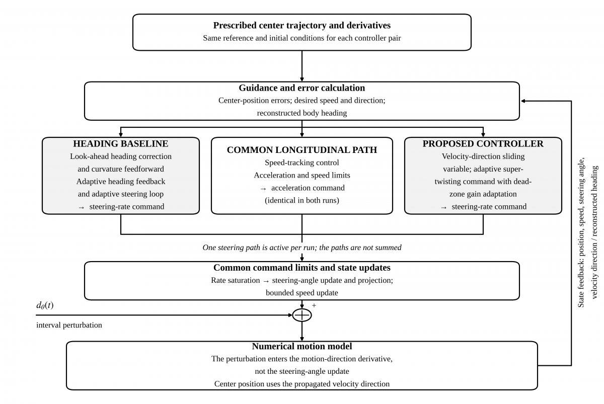
Figure 2. Signal flow of the numerical S0–S4 comparison. Each run selects one steering controller; the motion-direction perturbation enters the numerical model
Arrows indicate forward signal flow, and the return arrow denotes numerical state feedback. The longitudinal path is common to both runs. Controller and disturbance definitions follow Section 6.1.
Table 2. Common robot, numerical, and actuator settings
|
Quantity |
Value |
Unit |
|
$L, l_{r}$ |
2.70, 1.20 |
m |
|
$T_{s}, T_{f}$ |
0.01, 32 |
s |
|
$L_{1}, L_{2}, L_{3}$ |
5, 5, 5 |
m |
|
$k_{x}, k_{y}, k_{v}$ |
1.10, 1.25, 2.20 |
$s^{-1}$ |
|
$\delta_{\max}$ |
50 |
degree |
|
$\omega_{\max}$ |
55 |
degree/s |
|
$a_{\max}$ |
2.0 |
$m/s^{2}$ |
|
$v_{\min}, v_{\max}$ |
0, 1.4 |
m/s |
|
$v \left( 0 \right), \delta \left( 0 \right)$ |
0.10, 0 |
m/s, rad |
|
$\omega_{d}$ |
0.55 |
rad/s |
|
$t_{\mathrm{on}}, t_{\mathrm{off}}$ |
8, 24 |
s |
Table 3. Unchanged parameters of the implemented controllers
|
Method |
Parameter |
Value |
|
Proposed |
$\lambda_{y}$ |
1.10 rad/m |
|
Proposed |
$k_{1,\min}, k_{2,\min}$ |
0.75, 0.95 |
|
Proposed |
$\gamma_{1}, \gamma_{2}$ |
0.45, 0.55 |
|
Proposed |
$\sigma_{1}, \sigma_{2}$ |
1.30, 1.55 $s^{-1}$ |
|
Proposed |
Adaptation dead zone |
0.04 rad |
|
Baseline |
$k_{\psi,\min}$ |
1.15 |
|
Baseline |
$k_{\delta,\min}$ |
3.90 $s^{-1}$ |
|
Baseline |
$\gamma_{\psi}, \sigma_{\psi}$ |
0.40, 1.35 |
|
Baseline |
$\gamma_{\delta}, \sigma_{\delta}$ |
0.30, 2.30 |
|
Baseline |
Lateral scale; look-ahead gain |
0.45; 0.65 |
|
Baseline |
Lateral correction gain |
0.55 |
|
Baseline |
Feedforward angle limit |
32.5 degree |
|
Baseline |
Look-ahead/feedforward speed floor |
0.20/0.20 m/s |
|
Baseline |
Heading/steering adaptation dead zones |
0.60/0.45 degree |
The implemented heading baseline combines a look-ahead-adjusted heading reference, curvature feedforward, lateral correction, adaptive heading feedback, and an adaptive steering loop. The heading error used internally includes the look-ahead correction and is therefore not simply the analytical assignment in Eq. (27). Its plotted gains are $k_{\psi}$ and $k_{\delta}$, not the super-twisting coefficients in Section 4.2. The proposed implementation uses the super-twisting command structure with a backward-difference lateral-error derivative and a 0.04 rad adaptation dead zone. Both algorithms are evaluated without modifying their code or tuning between scenarios.
The benchmark propagates $\theta_{v}$ directly and reconstructs $\psi$ from $\theta_{v} - \beta$, with angular wrapping. Its perturbation $d_{\theta}(t)$ enters the motion-direction derivative in Eq. (94); the steering angle is advanced from the commanded rate alone and projected to its limits. This defines the numerical experiment. It is not an equivalent coordinate implementation of the analytical steering-actuator disturbance in Eq. (16). Figure 2 summarizes the evaluated signal flow; only one steering realization is active in each run.
6.2 Reference maneuver and additional scenarios
The reference retains the original sequence of three straight segments and two opposite quarter-circle turns:
$\begin{array}{c}\mathrm{straight} \left( L_{1} \right) \to \text{left turn} \left( R_{c} \right) \to \mathrm{straight} \left( L_{2} \right) \\ \to \text{right turn} \left( R_{c} \right) \to \mathrm{straight} \left( L_{3} \right) \end{array}$ (93)
The original case S0 uses $R_{c} = 2.50$ m and $v_{d} = 0.65$ m/s. S1 changes only the turn radius to 3.00 m, reducing the arc-curvature magnitude from 0.4000 to 0.3333 $m^{-1}$. S2 changes only the reference speed to 0.70 m/s. S3 changes only the disturbance amplitude to 0.63 rad/s. S4 changes only the initial position and direction angle. Table 4 gives all five cases. These are variations within the same left-right path family, not five unrelated path families.
Table 4. Five paired scenarios with unchanged tuning
|
Case |
Variation |
$R_{c}; v_{d}; A_{d}$ |
$x \left( 0 \right), y \left( 0 \right); \theta_{v} \left( 0 \right)$ |
|
S0 |
Original |
2.50; 0.65; 0.42 |
−1.0, −0.8; 8 |
|
S1 |
Radius |
3.00; 0.65; 0.42 |
−1.0, −0.8; 8 |
|
S2 |
Speed |
2.50; 0.70; 0.42 |
−1.0, −0.8; 8 |
|
S3 |
Amplitude |
2.50; 0.65; 0.63 |
−1.0, −0.8; 8 |
|
S4 |
Initial error |
2.50; 0.65; 0.42
|
−1.5, −1.2; 15
|
The 32 s horizon covers both turns in every case but does not include the entire final straight. Reference durations are 35.1600 s in S0, S3, and S4; 37.5766 s in S1; and 32.6485 s in S2. The terminal error is consequently the error at the common evaluation time of 32 s, not the final error after completing the entire prescribed path.
6.3 Interval disturbance model
The numerical perturbation is added directly to the effective motion-direction derivative:
$\dot{\theta}_{v} = \frac{v}{L} \tan \delta \cos \beta + G \left( \delta \right) \omega_{\delta} + d_{\theta} \left( t \right)$ (94)
The same prescribed signal is used in each controller pair:
$d_{\theta} \left( t \right) = \left\{ \begin{array}{c}A_{d} \sin \left( \omega_{d} \left( t - t_{\mathrm{on}} \right) \right), t_{\mathrm{on}} \leq t \leq t_{\mathrm{off}}, \\ 0, \mathrm{otherwise}\end{array} \right.$ (95)
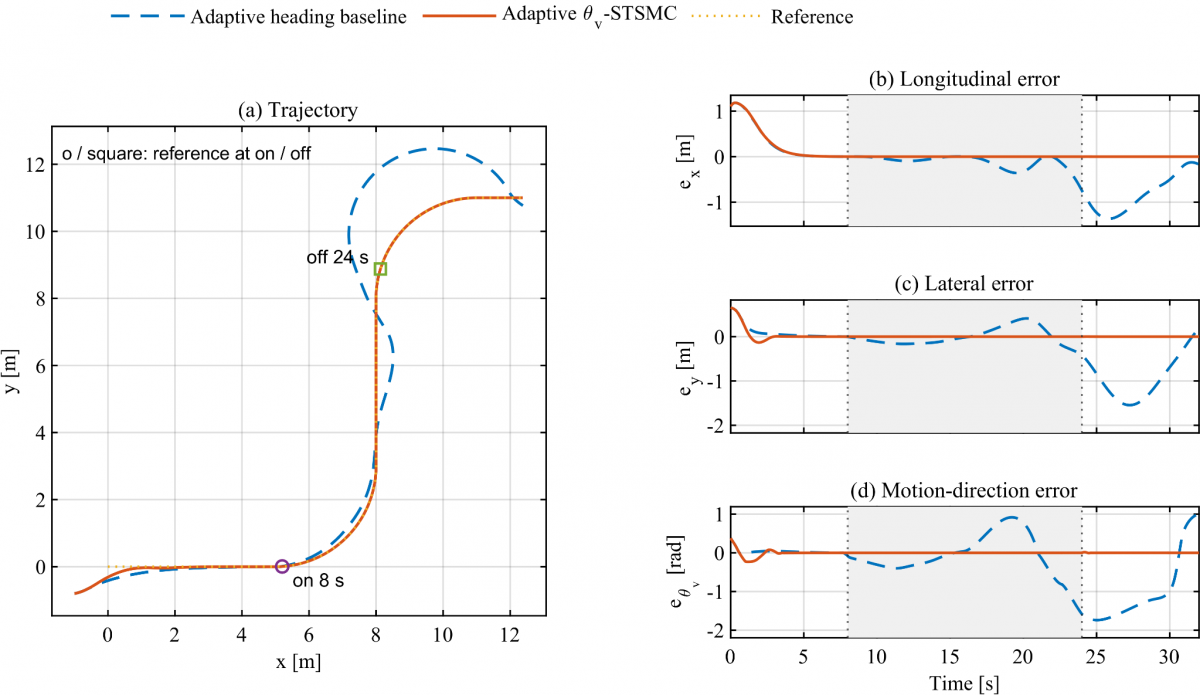
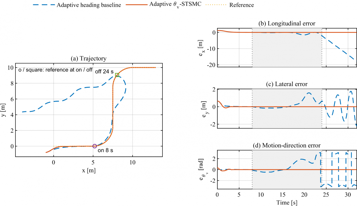
The amplitude is 0.42 rad/s in S0, S1, S2, and S4 and 0.63 rad/s in S3. The frequency is 0.55 rad/s and the active window is fixed at 8–24 s in every case. Thus the shaded band marks disturbance application, while 24–32 s shows recovery. Changing the radius or speed does not move this time window. The same prescribed $d_{\theta}(t)$ is applied to both controllers within each pair.
The bounded sinusoid is a deterministic matched-channel benchmark rather than an identified model of tire slip, wind loading, or actuator faults. It is smooth between switching instants but generally discontinuous at switch-off. A derivative bound required by an ideal super-twisting argument therefore applies only on the relevant smooth intervals. The 50% amplitude increase in S3 is a stronger test, not a demonstrated violation of a numerically certified disturbance bound.
6.4 Original actuator limits and controller parameters
The original angle and rate limits are unchanged: $\delta_{\max} = 50^{\circ}$ and $\omega_{\max} = 55^{\circ}$/s. The simulator clips the rate command and projects the next steering angle onto its admissible interval. The longitudinal acceleration is limited to 2.0 $m/s^{2}$, and the speed is restricted to 0–1.4 m/s. All additional cases retain these constraints; this dataset does not test changed actuator limits.
Baseline gains retain their actual source meanings. They are not renamed as the heading super-twisting gains of the analytical formulation. Complete original settings accompany the simulation files.
The parameter values in Table 3 are retained as the original design settings and are not optimized for S1–S4. The additional tests therefore examine transfer of one fixed tuning to changed operating conditions. The first and second proposed minimum gains retain positive square-root and auxiliary-integrator feedback even when the adaptive increments decay. Adaptation rates determine response to error above the dead zone, and leakage coefficients reduce the increments as the error subsides. These are the roles of the coefficients; neither numerical optimality nor a theorem-based sufficient-gain certificate is claimed.
For the baseline, the minimum heading-feedback and steering-loop gains have different functions from the proposed super-twisting coefficients. The original settings also include look-ahead correction, feedforward clipping, and separate adaptation dead zones. Common scenario inputs and unchanged parameters support a comparison of the two specified implementations, not a gain-normalized comparison. The numerical values and their preservation are documented; no original optimization record is available, and no retrospective optimization procedure is asserted.
6.5 Performance metrics and reproducibility
All performance indices use the complete 0–32 s record. The planar root-mean-square error (RMSE) is
$\mathrm{RMSE}_{p} = \sqrt{\frac{1}{T_{f}} \int_{0}^{T_{f}}\left[ \left( x_{d} - x \right)^{2} + \left( y_{d} - y \right)^{2} \right] d t}$ (96)
The lateral and effective velocity-direction errors are evaluated as
$\mathrm{RMSE}_{y} = \sqrt{\frac{1}{T_{f}} \int_{0}^{T_{f}}e_{y}^{2} d t}$ (97)
$\mathrm{RMSE}_{\theta_{v}} = \sqrt{\frac{1}{T_{f}} \int_{0}^{T_{f}}e_{\theta_{v}}^{2} d t}$ (98)
The final position error and steering-rate effort are
$e_{p,f} = \sqrt{\left( x_{d} \left( T_{f} \right) - x \left( T_{f} \right) \right)^{2} + \left( y_{d} \left( T_{f} \right) - y \left( T_{f} \right) \right)^{2}}$ (99)
$J_{\omega} = \int_{0}^{T_{f}}\omega_{\delta}^{2} d t$ (100)
The peak commanded steering rate is
$\omega_{\delta,\max} = \underset{0 \leq t \leq T_{f}}{\max} \left| \omega_{\delta} \left( t \right) \right|$ (101)
The integrals use trapezoidal quadrature. $J_{\omega}$ is an integrated steering-rate command index with units $\mathrm{rad}^{2}/s$, not electrical or mechanical energy. Error reduction is calculated from full-precision values as $100 \left( H - V \right)/H$, where H denotes the implemented adaptive heading baseline and V denotes the proposed adaptive velocity-direction controller. These are deterministic comparisons, not statistical significance tests.
All metrics are calculated from the state and command histories of the corresponding run. Identical scenario inputs, reference histories, initial conditions, and numerical settings are used for each controller pair. Reproduction of S0 and unchanged non-scenario settings provide a regression check for the additional-case evaluation. This establishes numerical consistency, not equivalence between the numerical benchmark and the analytical reference models.
6.6 Quantitative comparison across S0–S4
The proposed controller has lower planar, lateral, and velocity-direction RMSE and lower integrated steering-rate effort in every tested pair. The additional-case planar reductions range from 50.01% to 94.94%; effort reductions range from 7.81% to 44.39%. Tables 5–7 report every scenario, including the heading baseline’s loss of accurate tracking in S3, rather than selecting only successful outcomes.
Table 5. Tracking errors over 0–32 s
|
Case |
Method |
Planar RMSE (m) |
Lateral RMSE (m) |
Direction RMSE (rad) |
|
S0 |
H |
0.892664 |
0.712759 |
0.722302 |
|
S0 |
V |
0.279642 |
0.093549 |
0.051525 |
|
S1 |
H |
0.774105 |
0.550759 |
0.775304 |
|
S1 |
V |
0.279642 |
0.093549 |
0.051512 |
|
S2 |
H |
0.994597 |
0.805536 |
0.704990 |
|
S2 |
V |
0.291346 |
0.093646 |
0.062801 |
|
S3 |
H |
5.521227 |
0.695243 |
1.709197 |
|
S3 |
V |
0.279642 |
0.093550 |
0.051598 |
|
S4 |
H |
0.977003 |
0.713597 |
0.722014 |
|
S4 |
V |
0.488440
|
0.106711
|
0.042037
|
Table 6. Terminal error and steering-rate effort
|
Case |
Method |
Final Position Error (m) |
$J_{\omega}$ ($\mathrm{rad}^{2}/s$) |
|
S0 |
H |
0.391039 |
4.935291 |
|
S0 |
V |
$3.0117 \times 10^{-6}$ |
4.054062 |
|
S1 |
H |
0.248092 |
4.790147 |
|
S1 |
V |
$7.3944 \times 10^{-6}$ |
3.770714 |
|
S2 |
H |
0.573659 |
5.286197 |
|
S2 |
V |
$1.2208 \times 10^{-5}$ |
4.873173 |
|
S3 |
H |
17.855525 |
10.855649 |
|
S3 |
V |
$4.3041 \times 10^{-6}$ |
6.036782 |
|
S4 |
H |
0.391195 |
5.005699 |
|
S4 |
V |
$8.5518 \times 10^{-6}$
|
3.786708
|
Table 7. Reduction relative to the adaptive heading baseline
|
Case |
Planar RMSE |
Lateral RMSE |
Direction RMSE |
Steering Effort |
|
S0 |
68.67% |
86.88% |
92.87% |
17.86% |
|
S1 |
63.88% |
83.01% |
93.36% |
21.28% |
|
S2 |
70.71% |
88.37% |
91.09% |
7.81% |
|
S3 |
94.94% |
86.54% |
96.98% |
44.39% |
|
S4 |
50.01%
|
85.05%
|
94.18%
|
24.35%
|
The near-equal proposed planar RMSE values in S0, S1, and S3 have a direct numerical explanation. Those runs share the same initial condition, and their 0–8 s startup transient accounts for more than 99.999% of the full-horizon planar squared-error integral in each run. The remaining trajectory errors are small enough that the whole-horizon RMSE rounds to the same six-decimal value. This does not imply identical trajectories or disturbances: the radius changes in S1, the amplitude changes in S3, and their steering-rate effort and direction-error metrics differ. The full-horizon values are retained alongside the scenario-wise histories rather than replacing them with a selectively shortened error window.
6.7 Scenario-wise tracking, steering, and gain histories
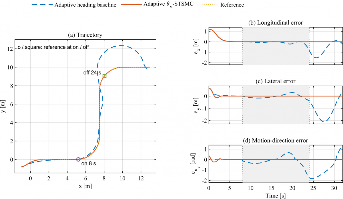
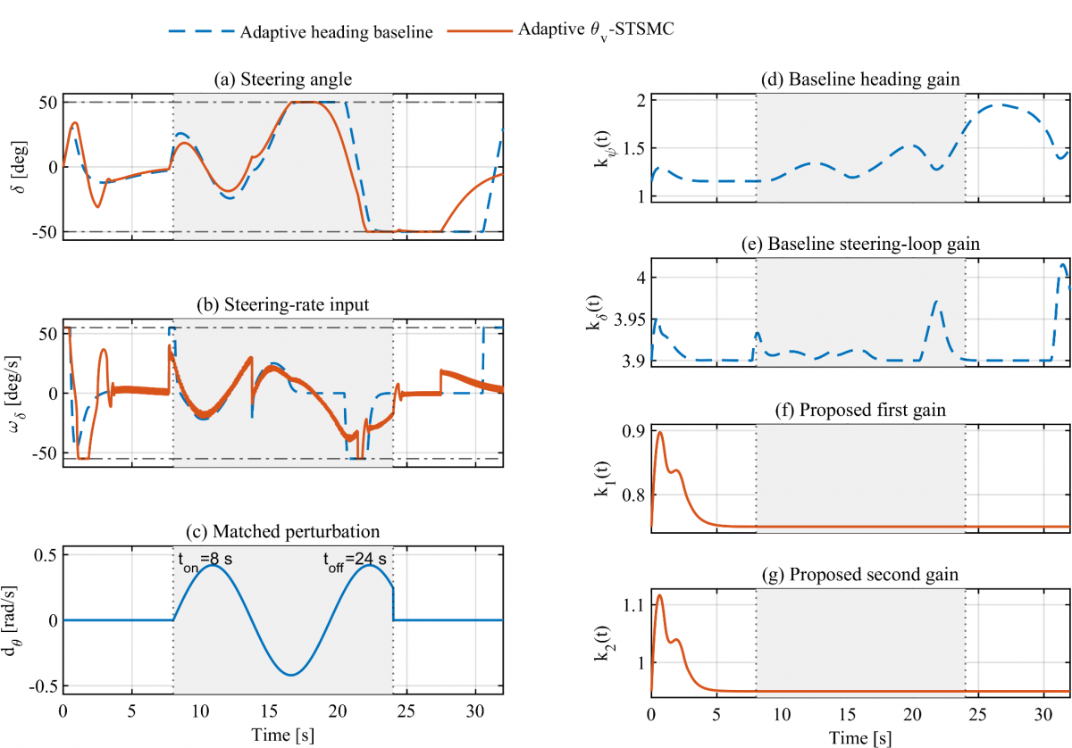
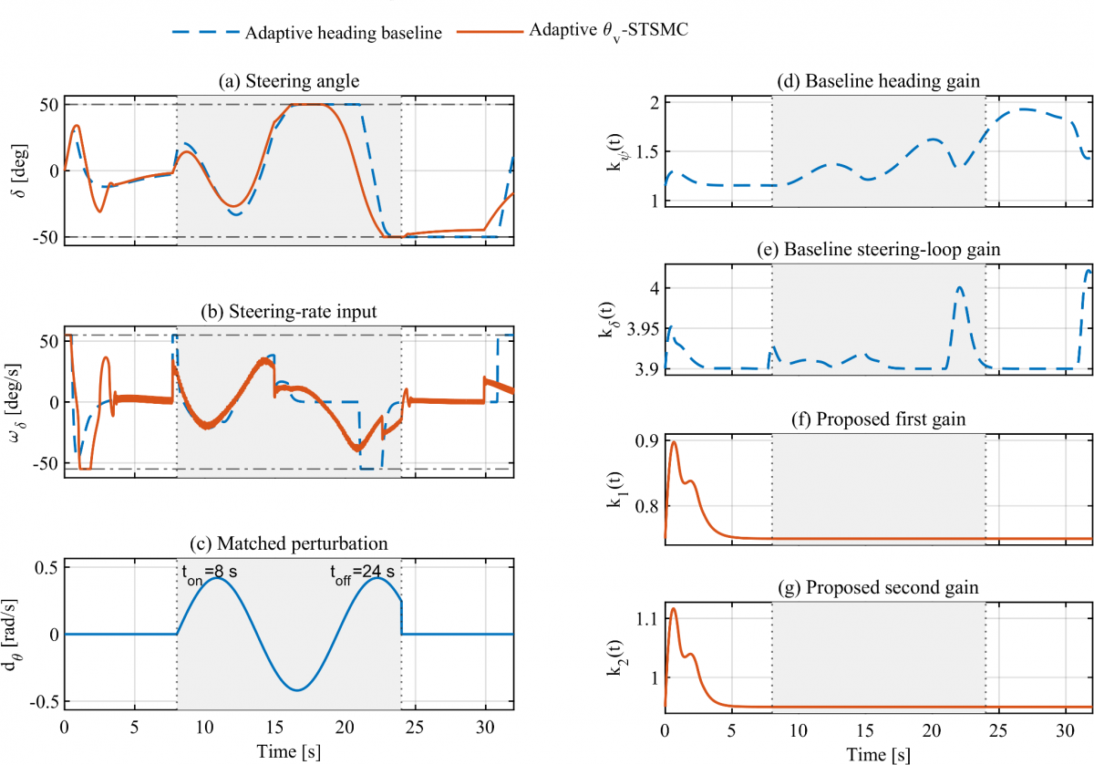
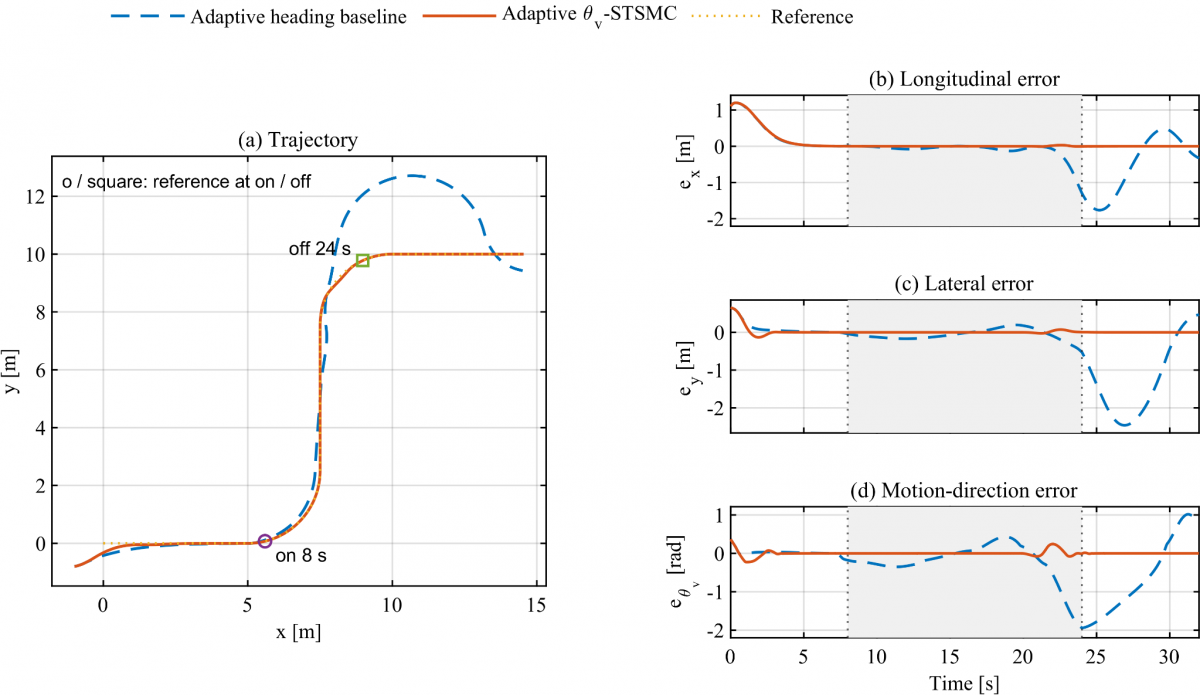
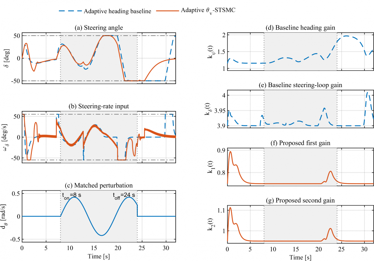
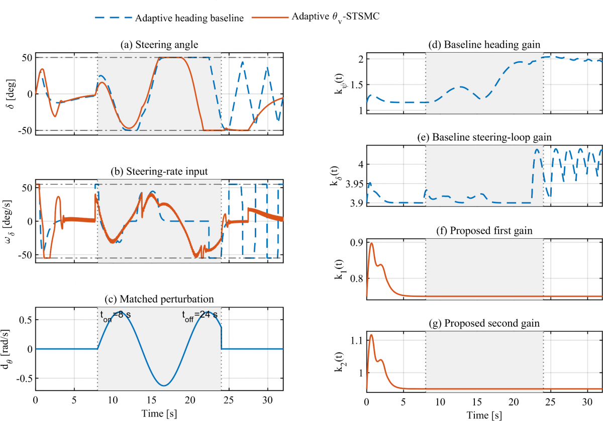
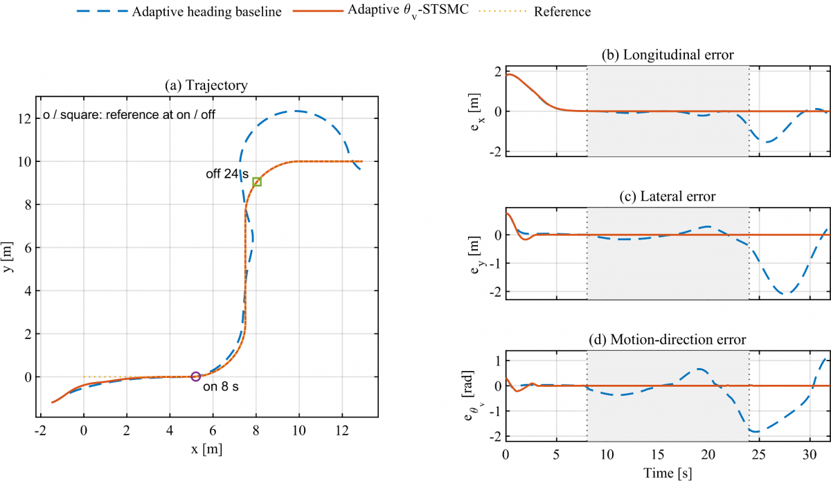
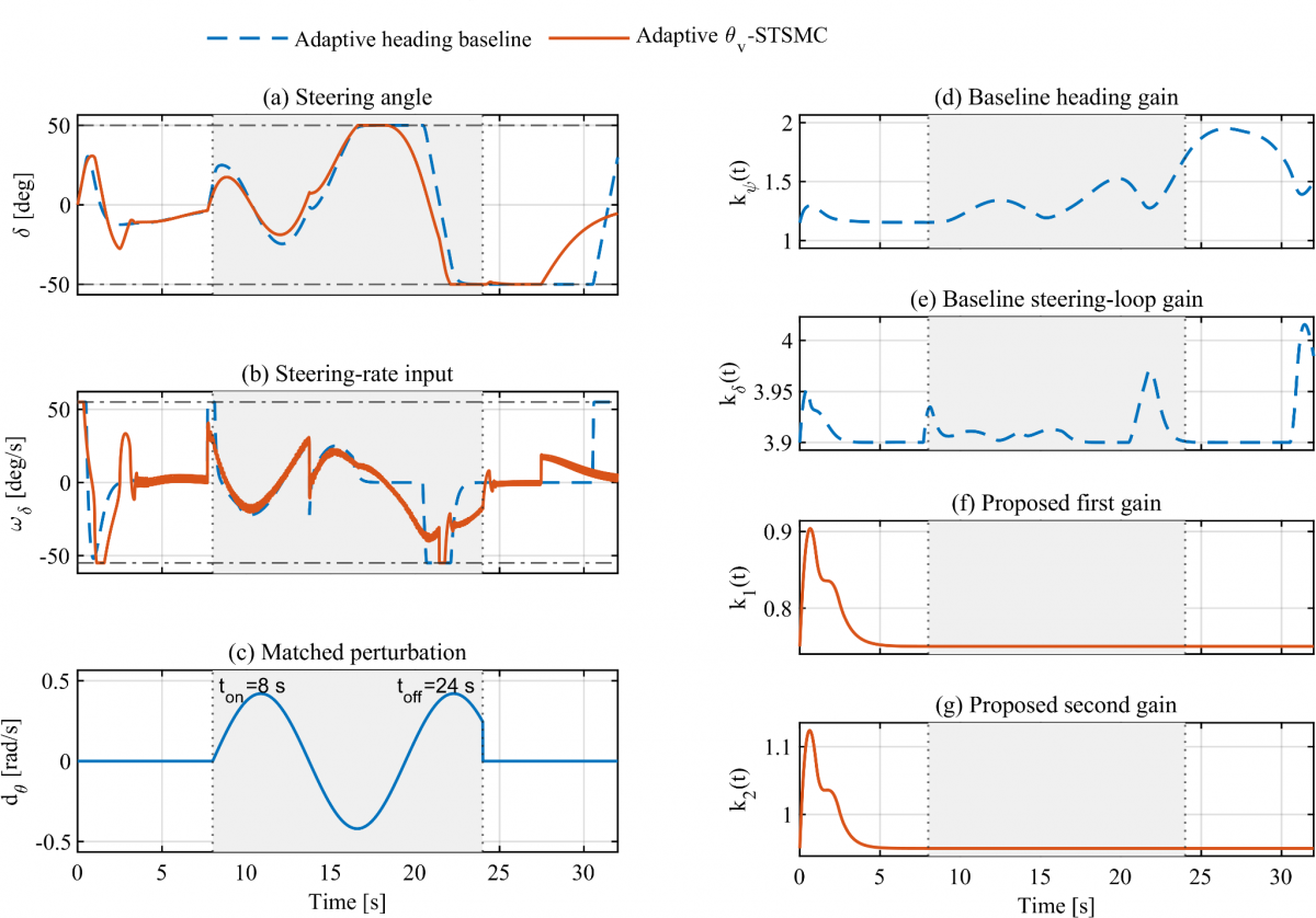
Two grouped figures are used for each scenario. The first shows the trajectory and three error histories; the second shows steering angle, rate input, the perturbation $d_{\theta}(t)$, and four adaptive-gain histories. The 8–24 s interval is marked consistently on the time axes. On each trajectory, the circle and square identify reference-path locations at disturbance onset and switch-off, rather than the simultaneous positions of both vehicles.
6.7.1 Original case S0
Figures 3 and 4 reproduce the original numerical comparison. The proposed trajectory remains close to the reference during the turns, whereas the baseline develops a pronounced second-turn and recovery deviation. Planar RMSE decreases from 0.892664 to 0.279642 m (68.67%), and steering-rate effort decreases from 4.935291 to 4.054062 $\mathrm{rad}^{2}/s$ (17.86%). The baseline’s final position error is 0.391039 m, compared with $3.0117 \times 10^{-6}$ m for the proposed method in this simulation.
Figure 3. S0 tracking performance. STSMC: super-twisting sliding-mode control; shaded interval: 8–24 s
Figure 4. S0 steering signals and gains. STSMC: super-twisting sliding-mode control; shaded interval: 8–24 s
6.7.2 Changed curvature S1
Figures 5 and 6 use a 3.00 m turn radius with all other settings unchanged. The proposed method retains close trajectory tracking. Planar RMSE decreases from 0.774105 to 0.279642 m (63.88%); lateral and direction RMSE reductions are 83.01% and 93.36%. Steering-rate effort decreases by 21.28%. This case extends the original comparison to a smaller curvature magnitude within the same maneuver family.
Figure 5. S1 tracking performance. STSMC: super-twisting sliding-mode control; shaded interval: 8–24 s
Figure 6. S1 steering signals and gains. STSMC: super-twisting sliding-mode control; shaded interval: 8–24 s
6.7.3 Higher reference speed S2
Figures 7 and 8 raise the reference speed to 0.70 m/s. A localized proposed-controller transient near the second turn is accompanied by temporary gain increases, after which the error decreases. Its planar RMSE is 0.291346 m versus 0.994597 m for the baseline (70.71% lower). The effort reduction is 7.81%, the smallest in this set; improved tracking therefore does not imply an identical effort advantage at every operating point.
Figure 7. S2 tracking performance. STSMC: super-twisting sliding-mode control; shaded interval: 8–24 s
Figure 8. S2 steering signals and gains. STSMC: super-twisting sliding-mode control; shaded interval: 8–24 s
6.7.4 Stronger disturbance S3
Figures 9 and 10 increase the disturbance amplitude by 50%, from 0.42 to 0.63 rad/s. The baseline loses accurate tracking and does not recover within the displayed horizon; its planar RMSE is 5.521227 m and its terminal error is 17.855525 m. The proposed method has planar RMSE 0.279642 m and terminal error $4.3041 \times 10^{-6}$ m. Its steering-rate effort increases to 6.036782 $\mathrm{rad}^{2}/s$ relative to S0, but remains 44.39% below the baseline in this pair. The result describes finite-horizon tracking loss, not an asymptotic-instability proof.
Figure 9. S3 tracking performance. STSMC: super-twisting sliding-mode control; shaded interval: 8–24 s
Figure 10. S3 steering signals and gains. STSMC: super-twisting sliding-mode control; shaded interval: 8–24 s
6.7.5 Larger initial tracking error S4
Figures 11 and 12 start at $\left(x, y \right) = \left(-1.5,-1.2 \right)$ m and $\theta_{v} = 15^{\circ}$. Both runs show a larger startup transient. The proposed method subsequently retains close corner tracking, with planar RMSE 0.488440 m versus 0.977003 m (50.01% lower), lateral RMSE 85.05% lower, and steering-rate effort 24.35% lower. The larger proposed planar RMSE than in S0 is consistent with the increased initial offset.
Figure 11. S4 tracking performance. STSMC: super-twisting sliding-mode control; shaded interval: 8–24 s
Figure 12. S4 steering signals and gains. STSMC: super-twisting sliding-mode control; shaded interval: 8–24 s
6.8 Gain interpretation and constraint activity
The gain histories retain their distinct definitions: the baseline uses $k_{\psi}$ and $k_{\delta}$, whereas the proposed method uses $k_{1}$ and $k_{2}$. Their S0 peaks are 1.949535, 4.015572, 0.897369, and 1.116637, respectively. The proposed gains have smaller numerical values in this comparison, but their different positions in the feedback laws prevent interpreting that fact alone as a normalized measure of control effort. The corresponding command-demand evidence is the steering-rate history and its integral index $J_{\omega}$, which is lower for the proposed method in every tested pair.
Both methods reach the fixed steering-angle and rate limits in S0–S4, with recorded peak magnitudes approximately 0.872665 rad and 0.959931 rad/s. Saturation is therefore active in the presented evidence, rather than an unused model feature. In S3, the stronger perturbation increases steering activity, but the unchanged bounds restrict further correction. These results characterize tracking under the selected limits. They do not measure the sensitivity of either controller to changing the limit values, and the larger S3 disturbance is not proof of rejection beyond a certified admissible range.
Changing an input bound would alter the admissible command and, for the angle bound, the nominal turning capability; it can therefore change both recovery and the effect of saturation. That influence is discussed qualitatively here. No changed-limit response or disturbance-rejection threshold is inferred from the fixed-limit S0–S4 dataset.
The S0–S4 results show a consistent separation between the implemented controllers across changes in curvature, speed, disturbance amplitude, and initial error. The proposed velocity-direction controller yields smaller tracking errors and lower integrated steering-rate effort in each pair, without case-specific retuning. This is the main numerical finding. The interpretation concerns the adaptive heading-feedback comparator and motion-direction perturbation specified in Section 6, rather than the unsimulated analytical heading reference.
The disturbance and recovery intervals play different roles. Several baseline responses develop their largest position deviations after the disturbance is switched off at 24 s, demonstrating that recovery cannot be assessed from the active-window error alone. In S3, the baseline position error is dominated by longitudinal deviation; a lateral-error metric alone would hide the severity of the tracking loss. Planar error, terminal error, and steering histories should therefore be interpreted together. The direction-error jumps in S3 also reflect angular wrapping and should not be read as instantaneous physical rotations.
The center-based kinematic interpretation is unchanged: the velocity vector points along $\theta_{v} = \psi + \beta$. This provides the motivation for regulating velocity direction. It does not by itself prove that every heading-based design must perform worse, because reference compensation, feedback realization, and tuning also affect the response. For the nominal geometric relations, the center velocity is
$v = v \left[ \begin{array}{c}\cos \theta_{v} \\ \sin \theta_{v}\end{array} \right]$ (102)
Differentiation gives
$\dot{v} = \dot{v} \left[ \begin{array}{c}\cos \theta_{v} \\ \sin \theta_{v}\end{array} \right] + v \dot{\theta}_{v} \left[ \begin{array}{c}-\sin \theta_{v} \\ \cos \theta_{v}\end{array} \right]$ (103)
Its normal acceleration and the associated qualitative inertial-force interpretation are
$a_{\perp} = v \dot{\theta}_{v}$ (104)
$F_{\perp} = \mathrm{mv} \dot{\theta}_{v}$ (105)
For locally circular motion,
$F_{\perp} = m \frac{v^{2}}{R}$ (106)
Here $m$ is robot mass and $R$ is the instantaneous center-path radius. These are kinematic relations, not an actuator-power or dynamic tire model. The reported $J_{\omega}$ therefore measures steering-command activity only; electrical energy, motor torque, and mechanical loading are not established by these simulations.
For low-speed automated transport or service robots, the engineering value of these tests is the observed reduction in center-path deviation and improved recovery with the selected steering authority. A system designer must assess the tracking tolerance together with the rate command, steering angle, and saturation duration, because a bounded input can coexist with unacceptable position error. S2 shows that increased speed can produce a localized transient even when aggregate tracking remains better; S3 shows that unchanged limits can coincide with severe baseline recovery failure.
At system level, trajectory generation should be coordinated with steering-angle and steering-rate capability rather than assuming that larger gains can compensate for infeasible commands. The implemented controller also requires center-position, velocity direction or reconstructed heading, steering angle, and a lateral-error derivative. A physical realization would need a consistent estimator and a measured steering actuator, and would have to account for differentiation noise and servo delay. The current plots characterize commanded motion, not motor current, torque, heating, or electrical energy. The very small simulated terminal errors are therefore numerical tracking results, not physical positioning specifications.
The evidence remains limited to one parameterized cornering-path family, deterministic sinusoidal motion-direction perturbations, exact-state feedback, fixed geometry, and fixed actuator settings. No physical robot or Robot Operating System/Gazebo validation is reported. Tire dynamics, measurement noise, delay, and input-limit sensitivity are not evaluated. The numerical findings therefore support the stated finite set of operating conditions, while the ideal analytical reference retains its separate assumptions and validation scope.
A velocity-direction-based adaptive super-twisting controller was evaluated against an adaptive heading-feedback baseline in five paired cornering scenarios with unchanged tuning. The original S0 comparison retains reductions of 68.67%, 86.88%, and 92.87% in planar, lateral, and velocity-direction root-mean-square errors and 17.86% in integrated steering-rate effort. The additional curvature, speed, disturbance-amplitude, and initial-error cases give planar-error reductions of 63.88%, 70.71%, 94.94%, and 50.01%, respectively, with lower integrated steering-rate effort in every pair. The stronger-disturbance case reveals loss of accurate baseline tracking and emphasizes post-disturbance recovery. These findings support the proposed implementation within the tested model and conditions. The numerical heading-feedback baseline and motion-direction disturbance remain distinct from the analytical steering-rate reference formulations. Further validation should examine actuator-limit sensitivity, sensing, tire dynamics, and physical implementation; the present data do not establish universal superiority or a global convergence guarantee.
During preparation and revision, ChatGPT (OpenAI) assisted with language editing, manuscript organization, MATLAB workflow support, numerical consistency checks, and figure arrangement. The author executed the native MATLAB simulations and is responsible for reviewing and approving the data, manuscript, and conclusions.
[1] Campion, G., Bastin, G., d’Andréa-Novel, B. (1996). Structural properties and classification of kinematic and dynamic models of wheeled mobile robots. IEEE Transactions on Robotics and Automation, 12(1): 47-62. https://doi.org/10.1109/70.481750
[2] De Luca, A., Oriolo, G., Samson, C. (2005). Feedback control of a nonholonomic car-like robot. In Robot Motion Planning and Control, pp. 171-253. https://doi.org/10.1007/BFb0036073
[3] Laumond, J.P. (1998). Robot Motion Planning and Control. Springer Nature. https://doi.org/10.1007/bfb0036069
[4] Siegwart, R., Nourbakhsh, I.R., Scaramuzza, D. (2011). Introduction to Autonomous Mobile Robots. MIT Press, Cambridge, MA.
[5] Paden, B., Čáp, M., Yong, S.Z., Yershov, D., Frazzoli, E. (2016). A survey of motion planning and control techniques for self-driving urban vehicles. IEEE Transactions on Intelligent Vehicles, 1(1): 33-55. https://doi.org/10.1109/tiv.2016.2578706
[6] Wang, C., Wang, D., Pan, W., Zhang, H. (2021). Output-based tracking control for a class of car-like mobile robot subject to slipping and skidding using event-triggered mechanism. Electronics, 10(23): 2886. https://doi.org/10.3390/electronics10232886
[7] Zhu, C., Li, B., Zhao, C., Wang, Y. (2024). Trajectory tracking control of car-like mobile robots based on extended state observer and backstepping control. Electronics, 13(8): 1563. https://doi.org/10.3390/electronics13081563
[8] Jin, X., Wang, Q., Yan, Z., Yang, H. (2023). Nonlinear robust control of trajectory-following for autonomous ground electric vehicles with active front steering system. AIMS Mathematics, 8(5): 11151-11179. https://doi.org/10.3934/math.2023565
[9] Rajamani, R. (2012). Vehicle Dynamics and Control. Springer Nature. https://doi.org/10.1007/978-1-4614-1433-9
[10] Kong, J., Pfeiffer, M., Schildbach, G., Borrelli, F. (2015). Kinematic and dynamic vehicle models for autonomous driving control design. In 2015 IEEE Intelligent Vehicles Symposium (IV), Seoul, South Korea, pp. 1094-1099. https://doi.org/10.1109/IVS.2015.7225830
[11] Snider, J.M. (2009). Automatic Steering Methods for Autonomous Automobile Path Tracking. Technical Report CMU-RI-TR-09-08, Robotics Institute, Carnegie Mellon University, Pittsburgh, PA.
[12] Hoffmann, G.M., Tomlin, C.J., Montemerlo, M., Thrun, S. (2007). Autonomous automobile trajectory tracking for off-road driving: Controller design, experimental validation and racing. In 2007 American Control Conference, New York, NY, USA, pp. 2296-2301. https://doi.org/10.1109/ACC.2007.4282788
[13] Stotsky, A., Hu, X., Egerstedt, M. (1999). Sliding mode control of a car-like mobile robot using single-track dynamic model. IFAC Proceedings Volumes, 32(2): 605-610. https://doi.org/10.1016/s1474-6670(17)56103-0
[14] Hamerlain, F., Floquet, T., Perruquetti, W. (2013). Experimental tests of a sliding mode controller for trajectory tracking of a car-like mobile robot. Robotica, 32(1): 63-76. https://doi.org/10.1017/s0263574713000623
[15] Polack, P., Altché, F., d’Andréa-Novel, B., de La Fortelle, A. (2017). The kinematic bicycle model: A consistent model for planning feasible trajectories for autonomous vehicles? In 2017 IEEE Intelligent Vehicles Symposium (IV), Los Angeles, CA, USA, pp. 812-818. https://doi.org/10.1109/IVS.2017.7995816
[16] Salazar, M., Alessandretti, A., Aguiar, A.P., Jones, C.N. (2015). An energy efficient trajectory tracking controller for car-like vehicles using Model Predictive Control. In 2015 54th IEEE Conference on Decision and Control (CDC), Osaka, pp. 3675-3680. https://doi.org/10.1109/CDC.2015.7402789
[17] Borrelli, F., Falcone, P., Keviczky, T., Asgari, J., Hrovat, D. (2005). MPC-based approach to active steering for autonomous vehicle systems. International Journal of Vehicle Autonomous Systems, 3(2/3/4): 265-291. https://doi.org/10.1504/ijvas.2005.008237
[18] Falcone, P., Borrelli, F., Asgari, J., Tseng, H.E., Hrovat, D. (2007). Predictive active steering control for autonomous vehicle systems. IEEE Transactions on Control Systems Technology, 15(3): 566-580. https://doi.org/10.1109/tcst.2007.894653
[19] Brown, M., Funke, J., Erlien, S., Gerdes, J.C. (2017). Safe driving envelopes for path tracking in autonomous vehicles. Control Engineering Practice, 61: 307-316. https://doi.org/10.1016/j.conengprac.2016.04.013
[20] Utkin, V. (1977). Variable structure systems with sliding modes. IEEE Transactions on Automatic Control, 22(2): 212-222. https://doi.org/10.1109/tac.1977.1101446
[21] Utkin, V.I. (1992). Sliding Modes in Control and Optimization. Springer Nature. https://doi.org/10.1007/978-3-642-84379-2
[22] Edwards, C., Spurgeon, S.K. (1998). Sliding Mode Control: Theory and Applications. Taylor & Francis, London.
[23] Young, K., Utkin, V., Ozguner, U. (1999). A control engineer's guide to sliding mode control. IEEE Transactions on Control Systems Technology, 7(3): 328-342. https://doi.org/10.1109/87.761053
[24] Shtessel, Y., Edwards, C., Fridman, L., Levant, A. (2014). Sliding Mode Control and Observation. Springer Nature. https://doi.org/10.1007/978-0-8176-4893-0
[25] Levant, A. (1993). Sliding order and sliding accuracy in sliding mode control. International Journal of Control, 58(6): 1247-1263. https://doi.org/10.1080/00207179308923053
[26] Levant, A. (2003). Higher-order sliding modes, differentiation and output-feedback control. International Journal of Control, 76(9-10): 924-941. https://doi.org/10.1080/0020717031000099029
[27] Moreno, J.A., Osorio, M. (2012). Strict Lyapunov functions for the super-twisting algorithm. IEEE Transactions on Automatic Control, 57(4): 1035-1040. https://doi.org/10.1109/tac.2012.2186179
[28] Plestan, F., Shtessel, Y., Brégeault, V., Poznyak, A. (2010). New methodologies for adaptive sliding mode control. International Journal of Control, 83(9): 1907-1919. https://doi.org/10.1080/00207179.2010.501385
[29] Shtessel, Y., Taleb, M., Plestan, F. (2012). A novel adaptive-gain supertwisting sliding mode controller: Methodology and application. Automatica, 48(5): 759-769. https://doi.org/10.1016/j.automatica.2012.02.024
[30] Utkin, V.I., Poznyak, A.S. (2013). Adaptive sliding mode control with application to super-twist algorithm: Equivalent control method. Automatica, 49(1): 39-47. https://doi.org/10.1016/j.automatica.2012.09.008
[31] Koubaa, Y., Boukattaya, M., Damak, T. (2018). Adaptive sliding mode control for trajectory tracking of nonholonomic mobile robot with uncertain kinematics and dynamics. Applied Artificial Intelligence, 32(9-10): 924-938. https://doi.org/10.1080/08839514.2018.1519100
[32] Oh, K., Seo, J. (2022). Development of a sliding-mode-control-based path-tracking algorithm with model-free adaptive feedback action for autonomous vehicles. Sensors, 23(1): 405. https://doi.org/10.3390/s23010405
[33] Ma, B., Pei, W., Zhang, Q. (2023). Trajectory tracking control of autonomous vehicles based on an improved sliding mode control scheme. Electronics, 12(12): 2748. https://doi.org/10.3390/electronics12122748
[34] Liu, W., Guo, R., Zhao, J. (2025). Adaptive sliding mode predictive control for path tracking of wheeled agricultural vehicles. Machines, 13(2): 157. https://doi.org/10.3390/machines13020157
[35] Vu, T.M., Moezzi, R., Cyrus, J., Hlava, J. (2021). Model predictive control for autonomous driving vehicles. Electronics, 10(21): 2593. https://doi.org/10.3390/electronics10212593
[36] Li, Z., Zhai, J. (2022). Super-twisting sliding mode trajectory tracking adaptive control of wheeled mobile robots with disturbance observer. International Journal of Robust and Nonlinear Control, 32(18): 9869-9881. https://doi.org/10.1002/rnc.6343
[37] Chen, C., Nie, J., Zhang, T., Li, Z., Shan, L., Huang, Z. (2023). Trajectory tracking control of super-twisting sliding mode of mobile robot based on neural network. Journal of Computational Methods in Sciences and Engineering, 23(1): 101-115. https://doi.org/10.3233/jcm-226507
[38] Yesmin, A., Nath, K., Kumari, K., Sinha, A., Bera, M.K. (2024). Adaptive generalized super-twisting sliding mode controller for wheeled mobile robot. IFAC-PapersOnLine, 57: 345-350. https://doi.org/10.1016/j.ifacol.2024.05.059
[39] Boubaker, S., Uliarte, J., Capraro, F., Kamel, S., Alsubaei, F.S., Bourennani, F., Rossomando, F. (2026). Adaptive and fractional-order super-twisting (FO-STA) control for trajectory tracking of mobile robots with differential traction. AIMS Mathematics, 11(5): 13589-13616. https://doi.org/10.3934/math.2026559
[40] Sun, J., Li, Q., Ding, S., Xing, G., Chen, L. (2023). Fixed-time generalized super-twisting control for path tracking of autonomous agricultural vehicles considering wheel slipping. Computers and Electronics in Agriculture, 213: 108231. https://doi.org/10.1016/j.compag.2023.108231
[41] He, Y., Wu, J., Xu, F., Liu, X., Wang, S., Cui, G. (2024). Path tracking control based on T-S fuzzy model for autonomous vehicles with yaw angle and heading angle. Machines, 12(6): 375. https://doi.org/10.3390/machines12060375
[42] Sun, Q., Zhu, K. (2024). Lateral controller for autonomous vehicle path tracking based on MPC-SMC dual model system. IEEE Access, 12: 187857-187867. https://doi.org/10.1109/access.2024.3514132
[43] Maaruf, M., Mysorewala, M.F. (2024). Neuro-adaptive path following control of autonomous ground vehicles with input deadzone. Discover Applied Sciences, 6(8): 415. https://doi.org/10.1007/s42452-024-06091-x
[44] Hosseinnajad, A., Mohajer, N., Rokonuzzaman, M. (2025). Double-surface homogeneous sliding mode control for self-driving cars. Nonlinear Dynamics, 113(21): 29511-29532. https://doi.org/10.1007/s11071-025-11632-z