
S Jayanthi | Zafar Ali Khan N | Suresh Kumar Natarajan* | J. Anitha Josephine | I. Ambika | C. Mahiba
© 2026 The authors. This article is published by IIETA and is licensed under the CC BY 4.0 license (http://creativecommons.org/licenses/by/4.0/).
OPEN ACCESS
Vision transformers (ViT) have become a leading approach for aerial scene classification. In the remote-sensing scene-classification literature, comparative studies of transformer architectures have often emphasized classification accuracy, with comparatively limited attention to statistical significance, computational efficiency, and feature representation. This study benchmarks five ViT variants: a generically pretrained plain transformer (ViT-B/16), a hierarchical windowed-attention model (Swin-V2-B), a self-supervised backbone (DINOv2), a masked-image-modeling backbone (EVA-02), and a remote-sensing-domain-pretrained model (RVSA), on the Aerial Image Dataset (AID) benchmark under a controlled fine-tuning and evaluation framework. Performance was assessed using standard classification metrics, paired statistical tests, computational profiling, feature-space analysis, and gradient-based interpretability. Swin-V2-B achieved the highest accuracy (98.55%), followed by ViT-B/16 (97.85%), RVSA (97.75%), EVA-02 (97.35%), and DINOv2 (97.15%). After multiple-comparison correction, only two of the ten pairwise comparisons were statistically significant, both involving Swin-V2-B against DINOv2 and EVA-02. Quantitative feature-space analysis indicated differences in class separability across architectures, with EVA-02 yielding the highest silhouette coefficient (0.837). Furthermore, SmoothGrad analysis showed that different architectures affect the visual regions involved in correct and misclassified predictions. Computational profiling further showed that lower theoretical FLOPs did not necessarily translate into lower inference latency. Specifically, window-based attention models exhibited higher per-image latency despite lower theoretical complexity. A supplementary experiment using a 20%-training-data protocol retained Swin-V2-B and DINOv2 as the highest- and lowest-ranked models, respectively, while RVSA and EVA-02 exchanged their relative positions. Ultimately, this study provides evidence to inform the selection of ViT for time-sensitive geospatial image-classification applications, including disaster-response mapping and operational land-cover mapping.
vision transformer, Swin Transformer, aerial scene classification, Aerial Image Dataset, remote sensing, statistical significance testing, land-use and land-cover
Land-use and land-cover (LULC) classification is crucial for interpreting high-resolution aerial and satellite imagery. This process supports many important activities, such as urban planning, disaster response, environmental monitoring, and geospatial intelligence [1-3]. Convolutional neural networks (CNNs) have long dominated visual recognition. However, the emergence of vision transformer (ViT) [4] demonstrated that transformer architectures based on self-attention can achieve competitive performance in large-scale image classification. This development has contributed to the broader adoption of transformer-based architectures for remote-sensing scene classification. Recent studies have further extended transformer-based remote-sensing classification toward reliability, uncertainty estimation, and interpretability, indicating a broader shift from accuracy-only evaluation toward more comprehensive assessment of model behavior [5]. The growing diversity of transformer architectures has consequently increased the need for systematic and multidimensional benchmarking. Existing comparative evaluations within remote-sensing scene classification have often emphasized aggregate predictive performance [6, 7], while less consistent attention has been given to statistical validation, computational profiling, quantitative feature-space analysis, and model interpretability [8, 9]. These considerations are particularly important for operational deployment, where computational requirements and inference efficiency can directly influence practical feasibility. Moreover, small differences in classification accuracy do not necessarily indicate statistically meaningful differences in predictive performance or practical deployment suitability.
To address this gap, this study conducts a comprehensive benchmark of five representative transformer-based architectures on the Aerial Image Dataset (AID). The objective is to evaluate predictive performance, alongside paired statistical validation, computational profiling, quantitative feature-space analysis, and gradient-based interpretability under a common evaluation framework. A supplementary evaluation under a reduced-training-data setting was also conducted to assess the sensitivity to training-data proportion of the comparative findings to training-data proportion. The five models were selected to represent three complementary dimensions of architectural and pretraining variation: (i) attention architecture, represented by vision transformer with 16 × 16 image patches (ViT-B/16) [4] and Swin Transformer V2-Base (Swin-V2-B) [10] (ii) pretraining paradigm, encompassing supervised ImageNet pretraining, self-supervised representation learning with DINOv2 ViT-B/14 [11], and masked image modeling (MIM) with knowledge distillation using EVA-02 ViT-B/14 [12] and (iii) pretraining domain, contrasting general-purpose ImageNet pretraining with remote-sensing-specific pretraining through Rotated Varied-Size Window Attention (RVSA-B), pretrained on MillionAID [13].
The contributions of this study are:
The remainder of this paper is organized as follows. Section 2 reviews related work in CNN- and transformer-based scene classification. Section 3 describes the dataset, model architectures, training protocol, and statistical and efficiency analysis methods. Section 4 presents the experimental results. Section 5 discusses their implications and limitations, and Section 6 concludes.
2.1 From convolutional to transformer-based aerial scene classification
Early deep learning approaches to aerial scene classification predominantly relied on CNN backbones fine-tuned on benchmark datasets such as UC Merced, AID, and NWPU-RESISC45 [1, 2, 14]. Xia et al. [1] reported baseline fine-tuning accuracies of 89.53% for CaffeNet, 89.64% for VGG-16, and 86.39% for GoogLeNet, under a 50/50 train/test split, providing early CNN baselines for aerial scene classification. Cheng et al. [2] further described the evolution of remote-sensing scene classification from handcrafted features and unsupervised feature learning toward end-to-end CNN-based methods.
The introduction of the ViT marked a major shift from CNN-based feature extraction by demonstrating that a transformer architecture based on global self-attention could achieve competitive performance in large-scale image classification [4]. This development contributed to the broader adoption of transformer-based models, including ViT and hierarchical architectures such as Swin Transformer. However, standard ViT applies global self-attention with quadratic complexity in the number of input tokens, which can increase computational cost as image resolution grows. Swin Transformer addressed this limitation through localized window-based self-attention with shifted windows, reducing the computational cost while enabling hierarchical feature representation [9, 15].
Subsequent studies have examined the effectiveness of transformer-based architectures for remote-sensing scene classification. Bashmal et al. [16] reported competitive performance of transformer-based models relative to conventional CNN architectures for remote sensing scene classification and highlighted the ability of self-attention to capture global contextual information. Similarly, Jannat and Willis showed that hierarchical Swin Transformers can improve remote-sensing image classification by integrating local texture information with broader contextual cues [17]. Review studies by Kumari and Kaul [18] and Maurício et al. [19] further summarized the growing adoption of transformer architectures across remote-sensing image-classification tasks and discussed their application across diverse downstream remote-sensing tasks. Zhang et al. [5] proposed TRS (Transformers for Remote Sensing Scene Classification), a hybrid CNN–Transformer architecture for remote-sensing scene classification. Recent remote-sensing studies have also continued to investigate transfer learning and pretrained deep-learning models for challenging land-cover classification problems [20].
Despite this progress, direct comparison of transformer architectures remains challenging because published results often use different datasets and experimental protocols. Such differences make it difficult to attribute observed performance differences specifically to architectural or pretraining choices.
2.2 Pretraining paradigms: Supervised, self-supervised, and masked image modeling
A second important dimension of variation concerns how a transformer backbone is pretrained prior to downstream fine-tuning. The ViT-B/16 and Swin-V2-B models considered in this study use supervised ImageNet pretraining. Self-supervised approaches learn visual representations from data without needing labeled data. DINOv2 employs self-distillation and was pretrained on the 142-million-image LVD-142M dataset [12]. The DINOv2 study reported strong transferability of the learned visual representations across diverse downstream tasks. A third paradigm, MIM, learns visual representations by predicting or reconstructing information from deliberately masked image regions. EVA-02 combines MIM with feature-level knowledge distillation from a large CLIP-derived teacher model [13].
These pretraining paradigms provide complementary mechanisms for learning visual representations, but their relative effectiveness for remote-sensing scene classification is difficult to isolate when studies use different datasets and evaluation protocols. A common downstream evaluation protocol is therefore useful for isolating the influence of pretraining strategy.
2.3 Remote-sensing-specific pretrained models
Remote-sensing-specific pretraining represents a further dimension of variation beyond general-purpose visual pretraining. Rather than learning exclusively from generic natural-image corpora, domain-specific foundation models are pretrained on remote-sensing imagery to capture characteristics such as spatial structure, scale variation, and scene diversity [21, 22]. RVSA represents this direction by adapting the ViT to remote-sensing imagery through rotated varied-size window attention and remote-sensing-specific pretraining [13]. Compared with general-purpose pretraining, domain-specific pretraining may provide representations better adapted to downstream remote-sensing tasks.
2.4 Methodological gaps in transformer benchmarking
Despite advances in transformer architectures and pretraining, important methodological gaps remain in how remote-sensing scene-classification models are comparatively evaluated. First, statistical significance testing is reported inconsistently across comparative remote-sensing scene-classification studies. McNemar’s test and the Wilcoxon signed-rank test provide established nonparametric approaches for complementary forms of paired model comparison [23, 24], but their use, together with appropriate multiple-comparison correction, is not consistently reported in remote-sensing scene-classification studies. Second, comparative analysis of model interpretability remains limited for this task. Hohl et al. reviewed interpretability approaches in remote sensing, with gradient- and perturbation-based methods for analyzing model decisions [25, 26]. However, attribution behavior across architecturally diverse transformer variants has received comparatively little attention.
Overall, the literature establishes the effectiveness of transformer-based models for remote-sensing scene classification, but systematic comparisons that jointly control architectural design, pretraining strategy, and pretraining domain while incorporating statistical, computational, representation-level, and interpretability analyses remain limited. These gaps motivate a controlled benchmark that jointly considers architectural variation, pretraining strategy, pretraining domain, statistical evidence, computational efficiency, representation structure, and model interpretability under a common evaluation protocol.
Figure 1 illustrates the overall workflow adopted in this study. The AID dataset [27] was partitioned into training, validation, and test subsets using a 70%/10%/20% split. Five ViT architectures, ViT-B/16, Swin-V2-B, DINOv2, EVA-02, and RVSA, were then fine-tuned under a common training and evaluation protocol to minimize variation arising from differences in experimental settings.
Following training, model performance was evaluated on the held-out test set using accuracy, precision, recall, and F1-score. The evaluation comprised four complementary analyses: (i) statistical analysis using bootstrap confidence intervals, McNemar's test, and Wilcoxon signed-rank test with multiple-comparison correction. (ii) computational profiling using model parameters, FLOPs, inference latency, GPU memory consumption, and Pareto analysis. (iii) feature representation analysis using t-distributed Stochastic Neighbor Embedding (t-SNE) and Uniform Manifold Approximation and Projection (UMAP) together by quantitative measures of class separability. (iv) gradient-based interpretability analysis using SmoothGrad saliency maps.
Figure 1. Workflow of the comparative benchmarking framework
To assess the sensitivity of the comparative findings to the amount of labeled training data and to enhance comparability with prior AID studies commonly using a 20% training-data setting, an additional experiment was conducted using 20% of the dataset for training, 10% for validation, and the remaining 70% for independent testing. The validation subset was kept separate from the test set to ensure that early stopping and checkpoint selection were performed without access to test data. The supplementary experiment followed the same model architectures, preprocessing configurations, and classification metrics as the primary benchmark.
3.1 Dataset description
Empirical evaluations were executed on the AID benchmark [27], which contains 10,000 RGB images spanning 30 distinct LULC scene classes. The images are 600 × 600 pixels and were collected from multiple remote-sensing sources with spatial resolutions ranging approximately from 0.5 to 8.0 m per pixel. The number of images per class ranges from approximately 220 to 420.
For the primary benchmark, a fixed stratified random split was used to create training, validation, and test subsets containing 70%, 10%, and 20% of the dataset, respectively. Stratification was used to preserve the class distribution across the subsets, and the three subsets were mutually exclusive. The split configuration is summarized in Table 1. The class-wise distributions are shown in Figure 2, and representative images from all 30 classes are presented in Figure 3.
The five transformer backbones were selected to represent different attention mechanisms and pretraining paradigms. Their principal architectural and pretraining characteristics are summarized in Table 2.
Figure 2. Class-wise image distribution across the training, validation, and test subsets
Figure 3. Representative images from the 30 scene classes from Aerial Image Dataset (AID)
Table 1. Aerial Image Dataset (AID) split summary
|
Split |
Images Count |
Proportion (%) |
|
Train |
7,000 |
70 |
|
Validation |
1,000 |
10 |
|
Test |
2,000 |
20 |
|
Total |
10,000 |
100.0 |
The models retain the input resolutions specified by their respective pretrained configurations. Swin-V2-B uses a 256 × 256 input, whereas ViT-B/16, DINOv2, EVA-02, and RVSA use 224 × 224 inputs. This difference is retained rather than artificially modifying the pretrained configurations. Consequently, input resolution is recognized as an experimental factor when interpreting differences in computational cost and predictive performance.
ViT-B/16 employs global multi-head self-attention to a sequence of non-overlapping 16 × 16 image patches. The backbone uses supervised pretraining on ImageNet-21K followed by fine-tuning on ImageNet-1K [4]. Swin-V2-B uses a hierarchical representation with shifted-window self-attention and was pretrained on ImageNet-21K [10]. Unlike global self-attention, window-based attention restricts computation to local regions, while shifted windows facilitate information exchange across neighboring windows. DINOv2 (ViT-B/14) represents the self-supervised pretraining paradigm. It employs self-distillation and was pretrained on the LVD-142M dataset, which contains approximately 142 million images [11]. The pretrained representation was transferred directly to the AID classification task without intermediate supervised ImageNet fine-tuning. EVA-02 (ViT-B/14) represents the MIM with feature-level knowledge distillation from a CLIP-derived vision teacher [12]. The evaluated backbone was pretrained using ImageNet-21K and transferred to the downstream AID classification task without intermediate supervised ImageNet fine-tuning. RVSA ViT-B represents the remote-sensing-specific pretraining paradigm. It employs Rotated Varied-Size Window Attention together with periodic global attention to model spatial patterns at different scales and orientations [13]. The backbone was pretrained using masked autoencoding on the MillionAID dataset [28]. For downstream AID classification, the pretrained classification head of each backbone was replaced with a randomly initialized fully connected layer containing 30 output units. All backbone parameters were subsequently fine-tuned.
All evaluated models build on the scaled dot-product self-attention mechanism. Given an input sequence of N tokens mapped to query (Q), key (K), and value (V) projections, the attention matrix is computed according to Eq. (1).
$Attention\left( Q,\text{ }\!\!~\!\!\text{ }K,\text{ }\!\!~\!\!\text{ }V \right)=softmax\left( \frac{Q{{K}^{T}}}{\surd d} \right)V$ (1)
where, d denotes the dimensionality of the key vectors.
The five backbones differ primarily in their attention organization and pretraining strategy, as summarized in Table 2.
Table 2. Structural and pretraining specifications of evaluated vision transformer (ViT) backbones
|
Model |
Attention Mechanism |
Pretraining Strategy |
Pretraining Dataset |
Input Size |
Parameters (M) |
|
ViT-B/16 |
Global self-attention |
Supervised |
ImageNet-21K, fine-tuned on ImageNet-1K |
$224\times 224$ |
85.82 |
|
Swin-V2-B |
Shifted window self-attention |
Supervised |
ImageNet-21K, fine-tuned on ImageNet-1K |
$256\times 256$ |
86.92 |
|
DINOv2 |
Global self-attention |
Self-supervised |
LVD-142M |
$224\times 224$ |
85.75 |
|
EVA-02 |
Global self-attention |
Masked image modeling (CLIP-distilled) |
ImageNet-21k |
$224\times 224$ |
85.78 |
|
RVSA |
Hybrid window/global attention |
Masked autoencoding |
MillionAID |
$224\times 224$ |
86.21. |
3.2 Training protocol
All five transformer backbones were fine-tuned using a common optimization protocol to minimize variation arising from differences in downstream training settings. The AdamW optimizer was used with a base learning rate of $1\times {{10}^{-4}}$, a weight decay of 0.05, and a batch capacity of 32 samples. A 3-epoch linear warm-up was followed by cosine learning-rate decay over the remaining training steps. Regularization included label smoothing with $\varepsilon =0.1$ and gradient-norm clipping at 1.0. Automatic mixed precision was used during training. Training was performed for a maximum of 30 epochs with early stopping based on validation accuracy and a patience of 15 epochs. The checkpoint achieving the highest validation accuracy was retained for subsequent evaluation. The held-out test set was not used for model selection or early stopping.
Label smoothing was incorporated into the cross-entropy objective. For an input with true class c, the regularized target vector ${{\tilde{y}}_{k}}\text{ }\!\!~\!\!\text{ }$is computed using Eq. (2).
$\tilde{y}_k=\left\{\begin{array}{c}1-\varepsilon+\frac{\varepsilon}{C}, \quad k=c \\ \frac{\varepsilon}{C}, \quad k \neq c\end{array}\right.$ (2)
where, $\varepsilon $ denotes thesmoothing factor and the total number of scene classes C is 30.
The corresponding cross-entropy loss is computed using Eq. (3).
$\mathcal{L}=-\sum_{k=1}^C \tilde{y}_k \log \left(p_k\right)$ (3)
where, ${{p}_{k}}$ denotes the predicted softmax probability for class k. The optimization step follows a segmented temporal learning rate function $\eta \left( t \right)$ as defined in Eq. (4).
$\eta(t)=\left\{\begin{array}{r}\eta_{\max } \frac{t}{t_w}, \quad t \leq t_w \\ \eta_{\max } \cdot \frac{1}{2}\left[1+\cos \left(\pi \frac{t-t_w}{t_{\max }-t_w}\right)\right],\end{array} \quad t>t_w\right.$ (4)
where, ${{\eta }_{max}}$ denotes the base learning rate, ${{t}_{w}}$ denotes the terminal step of the 3-epoch warmup, and ${{t}_{max}}$ denotes the total number of optimizer steps across a 30-epoch training horizon, and t denotes the current optimizer step. With a batch size of 32, tw corresponds to the number of mini-batch updates performed during the first three epochs.
3.3 Evaluation metrics and statistical analysis
Classification performance was evaluated using overall accuracy (OA) together with per-class precision, recall, and F1-score. OA was computed using Eq. (5).
$O A=\frac{1}{N} \sum_{i=1}^N I\left(y_i=\hat{y}_i\right)$ (5)
where, N denotes the number of test images, ${{y}_{i}}$ the ground-truth label, ${{\hat{y}}_{i}}$ the predicted label and $\mathrm{I}(\cdot)$ is the indicator function.
For each class c, precision, recall, and F1-score were computed using Eqs. (6)-(8) respectively.
$Precisio{{n}_{c}}=\frac{T{{P}_{c}}}{T{{P}_{c}}+F{{P}_{c}}}$ (6)
$Recal{{l}_{c}}=\frac{T{{P}_{c}}}{T{{P}_{c}}+F{{N}_{c}}}$ (7)
$F{{1}_{c}}=\frac{2Precisio{{n}_{c}}Recal{{l}_{c}}}{Precisio{{n}_{c}}+Recal{{l}_{c}}}$ (8)
where, $T{{P}_{c}},\text{ }\!\!~\!\!\text{ }F{{P}_{c}},\text{ }\!\!~\!\!\text{ and }\!\!~\!\!\text{ }F{{N}_{c}}$ denote the true-positive, false-positive, and false-negative counts for class c, respectively. Macro-averaged metrics were obtained by averaging the class-wise values equally across all 30 scene categories, whereas weighted averages accounted for the number of test samples in each class.
To assess pairwise differences between models, all statistical analyses were conducted using predictions or class-wise performance values derived from the same fixed, held-out test split. Three complementary statistical procedures were employed. First, bootstrap resampling was used to estimate the uncertainty of each model’s test accuracy. The test set was resampled with replacement 10,000 times, and the resulting distribution of bootstrap accuracies was used to compute percentile-based 95% confidence intervals. Second, McNemar's test was applied to all ten pairwise model comparisons using paired image-level correctness. For each model pair, the numbers of images correctly classified by model A but incorrectly classified by model B, and vice versa, were used to construct the paired 2 × 2 contingency table. When the total number of discordant observations was 25 or greater, the continuity-corrected McNemar chi-square statistic was used; when fewer than 25 discordant observations were present, the exact binomial version was applied. Let ${{n}_{10}}$ denote the number of test images correctly classified by model A but incorrectly classified by model B, and ${{n}_{01}}$ the reverse. For model pairs with at least 25 discordant observations, the continuity-corrected McNemar statistic was computed using Eq. (9).
${{\chi }^{2}}=\frac{{{(\left| {{n}_{10}}-{{n}_{01}} \right|-1)}^{2}}}{{{n}_{10}}+{{n}_{01}}}$ (9)
For model pairs with fewer than 25 discordant observations $({{n}_{10}}+{{n}_{01}}<25)$, the exact binomial version of McNemar's test was applied.
Third, pairwise Wilcoxon signed-rank tests were conducted using the classification accuracy of the 30 AID scene classes as the paired observations. The class-wise accuracy difference dc between models A and B was computed using Eq. (10).
${{d}_{c}}=Accuracy_{c}^{A}-Accuracy_{c}^{B}$ (10)
The corresponding Wilcoxon signed-rank statistic was computed using Eq. (11).
$W=\underset{c}{\mathop \sum }\,{{S}_{c}}{{R}_{c}}$ (11)
where, ${{R}_{c}}$ denotes the rank of $\left| {{d}_{c}} \right|$, and ${{S}_{c}}=sgn\left( {{d}_{c}} \right)$. Unlike McNemar's test, which evaluates paired image-level predictions, the Wilcoxon signed-rank test evaluates whether the class-wise performance differences are systematically shifted. Because ten pairwise model comparisons were conducted for each statistical test, Holm-Bonferroni correction was applied independently to both the McNemar and Wilcoxon test families to control the family-wise error rate at $\alpha =0.05$.
3.4 Computational efficiency analysis
Computational efficiency was evaluated using four complementary metrics that include total parameter count, FLOPs per image, inference latency, and peak GPU memory allocation during a single forward pass. FLOPs were estimated using Eq. (12).
$FLO{{P}_{S}}=2\times MA{{C}_{S}}$ (12)
The calculation follows the convention that one multiply-accumulate (MAC) operation consists of one multiplication and one addition and is therefore counted as two FLOPs.
Inference latency was measured on an NVIDIA RTX 3060 GPU using a batch size of one image. After ten warm-up iterations, inference time was averaged over 50 GPU-synchronized runs (R). Inference latency was computed using Eq. (13).
$Latency=\frac{1}{R}\underset{r=1}{\overset{R}{\mathop \sum }}\,{{t}_{r}},\text{ }\!\!~\!\!\text{ }r=1,\ldots ,R$ (13)
where, ${{t}_{r}}$ denotes the elapsed wall-clock inference time for run r. Reported latency values are presented as the mean $\pm $ standard deviation across the 50 runs. Peak GPU memory allocation was recorded during a single forward pass.
To characterize the trade-off between classification accuracy and computational cost, Pareto frontiers were constructed separately using FLOPs and measured inference latency as the cost metric. A model was considered Pareto-optimal if no other model achieved higher accuracy with equal or lower computational cost.
3.5 Interpretability analysis
To enable a consistent architecture-independent analysis, SmoothGrad [29], built upon vanilla input-gradient saliency [30], was employed. For an input image x and target-class score ${{f}_{c}}\left( x \right)$, vanilla saliency ${{M}_{c}}\left( x \right)$ is defined by Eq. (14).
${{M}_{c}}\left( x \right)=\frac{\partial {{f}_{c}}\left( x \right)}{\partial x}$ (14)
SmoothGrad was then computed by averaging the input gradients obtained from n = 20 Gaussian-noise perturbations, as defined in Eq. (15).
$\widehat{M}_c(x)=\frac{1}{n} \sum_{i=1}^n M_c\left(x+g_i\right), \quad g_i \sim N\left(0, \sigma^2 I\right)$ (15)
where, $\sigma =0.15$ denotes normalized pixel units. Averaging multiple noisy gradients reduces the visual noise commonly observed in single-gradient saliency maps while preserving the underlying discriminative regions. SmoothGrad does not directly expose internal attention weights; however, because it is based on input gradients, the same attribution procedure can be applied across all five architectures, providing a consistent basis for qualitative comparison.
4.1 Classification performance
Table 3 summarizes the classification performance of the five evaluated models on the AID test set across OA, macro precision, macro recall, macro F1, and weighted F1 score. In terms of OA, Swin-V2-B achieved the highest value of 98.55%, followed by ViT-B/16 (97.85%), RVSA (97.75%), EVA-02 (97.35%), and DINOv2 (97.15%). The macro F1 scores follow the same performance order, ranging from 0.9853 for Swin-V2-B to 0.9706 for DINOv2. The close agreement between OA and weighted F1 scores indicates consistent global performance. Conversely, the slightly lower macro-averaged scores reflect performance variation across the 30 scene classes.
Table 3. Summary of test-set performance bottom of form
|
Model |
Overall Accuracy |
Macro Precision |
Macro Recall |
Macro F1 |
Weighted F1 |
|
Swin-V2-B |
0.9855 |
0.9860 |
0.9849 |
0.9853 |
0.9855 |
|
ViT-B/16 |
0.9785 |
0.9784 |
0.9777 |
0.9779 |
0.9785 |
|
RVSA |
0.9775 |
0.9775 |
0.9767 |
0.9768 |
0.9775 |
|
EVA-02 |
0.9735 |
0.9736 |
0.9725 |
0.9726 |
0.9735 |
|
DINOv2 |
0.9715 |
0.9710 |
0.9706 |
0.9706 |
0.9714 |
Bootstrap 95% confidence intervals (Figure 4) ranged from approximately 0.964 to 0.991 across the five models. Swin-V2-B yielded the highest accuracy estimate with a 95% confidence interval of 0.980-0.991. This interval overlapped substantially with those of ViT-B/16 (0.972-0.985) and RVSA (0.971-0.984). Followed by ViT-B/16 (0.972-0.985), RVSA (0.971-0.984), EVA-02 (0.966-0.980), and DINOv2 (0.964-0.979).
Figure 4. Test accuracy with bootstrap 95% confidence intervals
4.2 Statistical significance
Pairwise McNemar's and Wilcoxon signed-rank tests were performed to examine differences between the five models, with Holm-Bonferroni correction applied separately to each set of ten pairwise comparisons. The results are presented in Table 4. After correction, McNemar's test indicated statistically significant differences in two comparisons, both involving Swin-V2-B: Swin-V2-B versus DINOv2 $(\rho H o l m=0.0039)$ and Swin-V2-B versus $\mathrm{EVA}-02(\rho \mathrm{Holm}=0.0081)$. The other pairwise comparisons did not reach statistical significance. The Wilcoxon signed-rank test, evaluated across the 30 scene classes, did not identify any statistically significant pairwise differences after correction. Table 5 reports the McNemar $\chi^2$ and Wilcoxon W statistics along with uncorrected $\rho$-values.
Table 4. Pairwise statistical test results after Holm-Bonferroni correction
|
Model A |
Model B |
McNemar $\rho H o l m$ |
Wilcoxon $\rho H o l m$ |
|
ViT-B/16 |
Swin-V2-B |
0.3636 |
0.6153 |
|
ViT-B/16 |
DINOv2 |
0.2796 |
0.5875 |
|
ViT-B/16 |
EVA-02 |
0.8827 |
1.0000 |
|
ViT-B/16 |
RVSA |
1.0000 |
1.0000 |
|
Swin-V2-B |
DINOv2 |
0.003922 |
0.0716 |
|
Swin-V2-B |
EVA-02 |
0.008108 |
0.0716 |
|
Swin-V2-B |
RVSA |
0.3151 |
0.4949 |
|
DINOv2 |
EVA-02 |
1.0000 |
1.0000 |
|
DINOv2 |
RVSA |
0.7079 |
0.8357 |
|
EVA-02 |
RVSA |
1.0000 |
1.0000 |
Table 5. Underlying McNemar and Wilcoxon test statistics with uncorrected p-values
|
Model A |
Model B |
McNemar χ² |
Raw p |
Wilcoxon W |
Raw p |
|
ViT-B/16 |
Swin-V2-B |
3.521 |
0.0606 |
26.5 |
0.1026 |
|
ViT-B/16 |
DINOv2 |
4.447 |
0.03496 |
40.0 |
0.08393 |
|
ViT-B/16 |
EVA-02 |
1.500 |
0.2207 |
76.5 |
0.4565 |
|
ViT-B/16 |
RVSA |
0.019 |
0.8897 |
101.0 |
0.8813 |
|
Swin-V2-B |
DINOv2 |
12.569 |
0.0003922 |
16.0 |
0.007160 |
|
Swin-V2-B |
EVA-02 |
11.021 |
0.0009009 |
29.0 |
0.007908 |
|
Swin-V2-B |
RVSA |
4.018 |
0.04502 |
69.0 |
0.06186 |
|
DINOv2 |
EVA-02 |
0.141 |
0.7077 |
111.0 |
0.8757 |
|
DINOv2 |
RVSA |
2.161 |
0.1416 |
68.0 |
0.1671 |
|
EVA-02 |
RVSA |
0.721 |
0.3960 |
95.0 |
0.4761 |
4.3 Error analysis
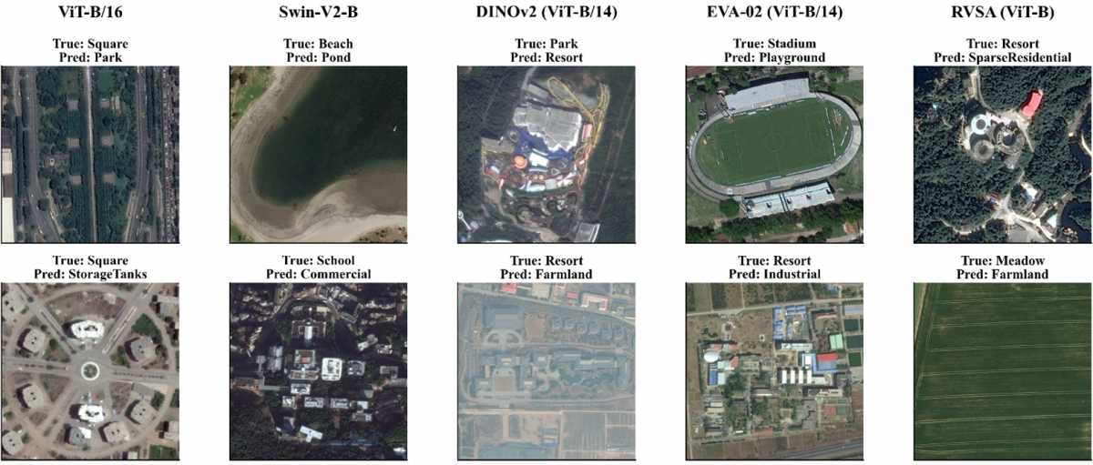
The row-normalized confusion matrices (Figure 5) indicate high overall classification performance across all models. All matrices are visually near-diagonal, with off-diagonal mass confined to faint, low-probability cells. In all matrices, no single class shows a severe, isolated failure mode for any architecture. Instead, the per-class precision and recall (Table 6) reveal a shared, moderate performance limitation common to all five models. This limitation is concentrated in the planned-facility classes, such as Resort, Commercial, and Church. All five models retain recall and precision above 0.84 for every evaluated class, showing a highly consistent performance envelope across architectures. For instance, Resort recall represents the weakest or near-weakest class performance for ViT-B/16 (0.897), DINOv2 (0.897), and RVSA (0.897). Similarly, EVA-02’s Resort recall (0.845) is its lowest value across all classes. While Swin-V2-B achieves a higher Resort recall (0.914), it exhibits its lowest precision on Commercial-adjacent confusions. These metrics indicate that planned-facility identification represents a consistently more difficult sub-problem for all evaluated architectures. Manual inspection of misclassified test examples (Figure 6) corroborates this pattern with concrete visual instances.
Figure 5. Row-normalized confusion matrices for the test set obtained using the five evaluated vision transformer (ViT) architectures: (a) ViT-B/16, (b) Swin-V2-B, (c) DINOv2 (ViT-B/14), (d) EVA-02 (ViT-B/14), (e) RVSA (ViT-B)
Figure 6. Representative misclassified test examples across all five architectures, with true and predicted labels
Table 6. Per-class precision/recall for the classes, showing the performance across models
|
Class |
ViT-B/16 P |
ViT-B/16 R |
ViT-B/16 F1 |
Swin-V2-B P |
Swin-V2-B R |
Swin-V2-B F1 |
DINOv2 P |
DINOv2 R |
DINOv2 F1 |
EVA-02 P |
EVA-02 R |
EVA-02 F1 |
RVSA P |
RVSA R |
RVSA F1 |
|
Airport |
0.986 |
0.972 |
0.979 |
1.000 |
0.986 |
0.993 |
0.972 |
0.972 |
0.972 |
0.986 |
0.986 |
0.986 |
0.960 |
1.000 |
0.980 |
|
BareLand |
1.000 |
0.984 |
0.992 |
1.000 |
0.984 |
0.992 |
0.967 |
0.952 |
0.959 |
0.984 |
0.984 |
0.984 |
0.983 |
0.952 |
0.967 |
|
BaseballField |
1.000 |
1.000 |
1.000 |
1.000 |
1.000 |
1.000 |
1.000 |
1.000 |
1.000 |
1.000 |
1.000 |
1.000 |
1.000 |
0.977 |
0.989 |
|
Beach |
0.986 |
1.000 |
0.993 |
1.000 |
1.000 |
1.000 |
0.986 |
0.986 |
0.986 |
0.986 |
1.000 |
0.993 |
0.986 |
1.000 |
0.993 |
|
Bridge |
0.984 |
0.969 |
0.976 |
0.984 |
0.984 |
0.984 |
0.969 |
0.969 |
0.969 |
0.969 |
0.984 |
0.976 |
0.969 |
0.984 |
0.976 |
|
Center |
0.984 |
1.000 |
0.992 |
1.000 |
1.000 |
1.000 |
0.984 |
0.984 |
0.984 |
1.000 |
0.984 |
0.992 |
0.984 |
0.984 |
0.984 |
|
Church |
0.986 |
1.000 |
0.993 |
1.000 |
0.986 |
0.993 |
0.986 |
0.986 |
0.986 |
1.000 |
0.986 |
0.993 |
0.986 |
1.000 |
0.993 |
|
Commercial |
1.000 |
0.984 |
0.992 |
1.000 |
1.000 |
1.000 |
0.984 |
0.984 |
0.984 |
1.000 |
0.984 |
0.992 |
0.984 |
0.984 |
0.984 |
|
DenseResidential |
0.986 |
1.000 |
0.993 |
0.986 |
1.000 |
0.993 |
0.986 |
0.984 |
0.985 |
1.000 |
0.986 |
0.993 |
0.986 |
0.986 |
0.986 |
|
Desert |
0.984 |
0.984 |
0.984 |
0.984 |
0.984 |
0.984 |
0.968 |
0.984 |
0.976 |
0.984 |
0.984 |
0.984 |
0.984 |
0.968 |
0.976 |
|
Farmland |
0.984 |
0.984 |
0.984 |
0.984 |
0.984 |
0.984 |
0.984 |
0.984 |
0.984 |
0.984 |
0.984 |
0.984 |
0.984 |
0.984 |
0.984 |
|
Forest |
1.000 |
0.984 |
0.992 |
1.000 |
1.000 |
1.000 |
0.984 |
1.000 |
0.992 |
1.000 |
0.984 |
0.992 |
0.984 |
1.000 |
0.992 |
|
Industrial |
0.984 |
0.984 |
0.984 |
1.000 |
0.984 |
0.992 |
0.984 |
0.984 |
0.984 |
0.984 |
0.984 |
0.984 |
0.984 |
0.984 |
0.984 |
|
Meadow |
1.000 |
0.984 |
0.992 |
1.000 |
1.000 |
1.000 |
0.984 |
0.984 |
0.984 |
0.984 |
1.000 |
0.992 |
0.984 |
1.000 |
0.992 |
|
MediumResidential |
0.984 |
0.984 |
0.984 |
1.000 |
0.984 |
0.992 |
0.984 |
0.984 |
0.984 |
0.984 |
0.984 |
0.984 |
0.984 |
0.984 |
0.984 |
|
Mountain |
1.000 |
0.984 |
0.992 |
1.000 |
1.000 |
1.000 |
0.984 |
0.984 |
0.984 |
1.000 |
0.984 |
0.992 |
0.984 |
0.984 |
0.984 |
|
Park |
0.984 |
1.000 |
0.992 |
1.000 |
0.984 |
0.992 |
0.984 |
0.984 |
0.984 |
1.000 |
0.984 |
0.992 |
0.984 |
1.000 |
0.992 |
|
Parking |
0.984 |
1.000 |
0.992 |
1.000 |
1.000 |
1.000 |
0.984 |
0.984 |
0.984 |
1.000 |
0.984 |
0.992 |
0.984 |
1.000 |
0.992 |
|
Playground |
1.000 |
0.984 |
0.992 |
1.000 |
1.000 |
1.000 |
0.984 |
0.984 |
0.984 |
1.000 |
0.984 |
0.992 |
0.984 |
0.984 |
0.984 |
|
Pond |
0.984 |
1.000 |
0.992 |
1.000 |
1.000 |
1.000 |
0.984 |
0.984 |
0.984 |
0.984 |
1.000 |
0.992 |
0.984 |
0.984 |
0.984 |
|
RailwayStation |
1.000 |
0.984 |
0.992 |
1.000 |
0.984 |
0.992 |
0.984 |
0.984 |
0.984 |
1.000 |
0.984 |
0.992 |
0.984 |
0.984 |
0.984 |
|
Resort |
0.984 |
0.984 |
0.984 |
1.000 |
0.984 |
0.992 |
0.984 |
0.984 |
0.984 |
0.984 |
0.984 |
0.984 |
0.984 |
0.984 |
0.984 |
|
River |
0.984 |
0.984 |
0.984 |
1.000 |
0.984 |
0.992 |
0.984 |
0.984 |
0.984 |
0.984 |
0.984 |
0.984 |
0.984 |
0.984 |
0.984 |
|
School |
0.984 |
1.000 |
0.992 |
1.000 |
1.000 |
1.000 |
0.984 |
0.984 |
0.984 |
1.000 |
0.984 |
0.992 |
0.984 |
0.984 |
0.984 |
|
SparseResidential |
1.000 |
0.984 |
0.992 |
1.000 |
0.984 |
0.992 |
0.984 |
0.984 |
0.984 |
1.000 |
0.984 |
0.992 |
0.984 |
0.984 |
0.984 |
|
Stadium |
1.000 |
0.984 |
0.992 |
1.000 |
1.000 |
1.000 |
0.984 |
0.984 |
0.984 |
1.000 |
0.984 |
0.992 |
0.984 |
0.984 |
0.984 |
|
StorageTanks |
0.984 |
0.984 |
0.984 |
1.000 |
0.984 |
0.992 |
0.984 |
0.984 |
0.984 |
0.984 |
0.984 |
0.984 |
0.984 |
0.984 |
0.984 |
|
TennisCourt |
1.000 |
1.000 |
1.000 |
1.000 |
1.000 |
1.000 |
0.984 |
0.984 |
0.984 |
1.000 |
1.000 |
1.000 |
1.000 |
0.984 |
0.992 |
|
Terrace |
0.984 |
0.984 |
0.984 |
1.000 |
0.984 |
0.992 |
0.984 |
0.984 |
0.984 |
0.984 |
0.984 |
0.984 |
0.984 |
0.984 |
0.984 |
|
TrainStation |
0.984 |
0.984 |
0.984 |
1.000 |
0.984 |
0.992 |
0.984 |
0.984 |
0.984 |
1.000 |
0.984 |
0.992 |
0.984 |
0.984 |
0.984 |
|
Viaduct |
0.984 |
0.984 |
0.984 |
1.000 |
0.984 |
0.992 |
0.984 |
0.984 |
0.984 |
0.984 |
0.984 |
0.984 |
0.984 |
0.984 |
0.984 |
A cluster of semantically related planned-facility classes, including Resort, Commercial, School, Center, and Square, recurs among the sampled errors for every architecture. Representative errors include Resort misclassified as SparseResidential or Industrial, Commercial as StorageTanks, and School as Commercial. Their similar spatial layouts, comprising organized building complexes and open paved areas, make them difficult to distinguish regardless of the underlying ViT architecture. The remaining sampled confusions, including Square-Park, Beach-Pond, Park-Resort, and Stadium-Playground, correspond to scene categories with overlapping structural characteristics rather than an architecture-specific weakness.
4.4 Efficiency and Pareto analysis
Computational efficiency was assessed using parameter count, FLOPs, measured inference latency, and peak GPU memory allocation. The corresponding results are reported in Table 7.
Table 7. Architectural hardware efficiency and resource footprint profile of the evaluated models
|
Model |
Params (M) |
GFLOPs |
Latency (ms) |
Peak VRAM (MB) |
|
ViT-B/16 |
85.82 |
33.73 |
9.40 ± 0.49 |
370.6 |
|
Swin-V2-B |
86.92 |
30.48 |
26.21 ± 3.17 |
438.2 |
|
DINOv2 |
85.75 |
43.93 |
11.75 ± 0.33 |
372.5 |
|
EVA-02 |
85.78 |
43.89 |
13.71 ± 0.24 |
375.8 |
|
RVSA |
86.21 |
33.56 |
27.64 ± 0.91 |
375.6 |
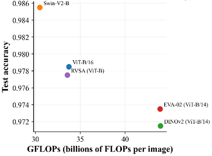
The five models exhibit comparable parameter counts, ranging from 85.75 to 86.92 million, while peak GPU memory allocation ranged from 370.6 to 438.2 MB at batch size one. In contrast, theoretical computational cost and measured inference latency showed different patterns across the models. Swin-V2-B required the fewest FLOPs (30.48 GFLOPs) but showed a measured latency of 26.21 ms per image. ViT-B/16 required 33.73 GFLOPs but achieved the lowest latency of 9.40 ms per image. DINOv2 and EVA-02 had the highest FLOPs (43.93 and 43.89 GFLOPs, respectively), with latencies of 11.75 and 13.71 ms per image, while RVSA required 33.56 GFLOPs and showed a latency of 27.64 ms per image. These results indicate that theoretical FLOPs did not consistently correspond to measured inference latency under the evaluated hardware and inference protocol.
Figure 7. Accuracy vs. GFLOPs Pareto frontier
To examine the trade-off between predictive performance and computational cost, Pareto frontiers were constructed using FLOPs and measured inference latency separately as cost metrics. When FLOPs are considered as the cost metric, Swin-V2-B is the single Pareto-optimal model, combining the highest test accuracy with the lowest GFLOP count (Figure 7). When measured inference latency is used as the cost metric, ViT-B/16 and Swin-V2-B lie on the latency-based Pareto frontier (Figure 8), reflecting a trade-off between prediction accuracy and runtime. The remaining models did not lie on the Pareto frontier. Overall, the relative efficiency of the evaluated models varied depending on whether FLOPs or measured inference latency was used as the cost metric.
Figure 8. Accuracy vs. measured inference latency Pareto frontier
4.5 Feature-space embeddings
To examine the organization of the learned representations, t-SNE and UMAP were applied to the pre-logit feature spaces of the held-out test images (Figures 9 and 10). Both dimensionality-reduction methods showed discernible class-wise organization across the five models. However, the degree of dispersion and overlap varied across architectures. ViT-B/16, Swin-V2-B, and EVA-02 generally exhibited relatively compact groupings for several classes. Conversely, RVSA showed greater dispersion and several elongated structures. DINOv2 showed generally identifiable class-wise groupings with some dispersion and overlap. These visual observations are qualitative. The geometry of t-SNE and UMAP projections depends heavily on hyperparameter configurations and algorithmic constraints. Since low-dimensional projections do not directly measure separation in the original feature space, quantitative metrics were computed directly from the uncompressed pre-logit feature vectors to preserve the true high-dimensional geometric relationships.
4.5.1 Quantitative class-separation metrics
The mean silhouette coefficient and the ratio of mean inter-class to mean intra-class Euclidean distance were computed from the pre-logit feature vectors of the held-out test set. The results are reported in Table 8.
Table 8. Quantitative class-separation metrics computed from pre-logit test-set features
|
Model |
Silhouette Coefficient |
Inter/Intra-Class Distance Ratio |
|
EVA-02 |
0.824 |
9.34 |
|
Swin-V2-B |
0.794 |
7.58 |
|
RVSA |
0.738 |
6.10 |
|
DINOv2 |
0.734 |
6.27 |
|
ViT-B/16 |
0.698 |
5.26 |
EVA-02 obtained the highest silhouette coefficient (0.824) and inter/intra-class distance ratio (9.34). Swin-V2-B followed with values of 0.794 and 7.58, respectively. RVSA and DINOv2 showed similar silhouette coefficients (0.738 and 0.734), while their inter/intra-class distance ratios were 6.10 and 6.27, respectively. ViT-B/16 obtained the lowest values for both measures. The feature-space measures did not follow the same ordering as classification accuracy reported in Table 3. In particularly, EVA-02 achieved the highest values for both class-separation measures, whereas Swin-V2-B achieved the highest test accuracy. ViT-B/16 also achieved higher test accuracy than EVA-02 despite obtaining a lower silhouette coefficient and inter/intra-class distance ratio. These results show that feature-space organization and classification accuracy provide complementary perspectives on model behaviour.
Figure 9. t-distributed Stochastic Neighbor Embedding (t-SNE) embeddings of pre- logit features for all five models: (a) ViT-B/16, (b) Swin-V2-B, (c) DINOv2 (ViT-B/14), (d) EVA-02 (ViT-B/14), (e) RVSA (ViT-B)
Figure 10. Uniform Manifold Approximation and Projection (UMAP) embeddings of pre-logit features for all five models: (a) ViT-B/16, (b) Swin-V2-B, (c) DINOv2 (ViT-B/14), (d) EVA-02 (ViT-B/14), (e) RVSA (ViT-B)
4.6 Interpretability
SmoothGrad saliency maps were examined for six representative test images to provide a qualitative comparison of the input regions highlighted by the five models (Figure 11). The evaluated examples include Viaduct, Farmland, Desert, Resort, Stadium, and Airport scenes. For a given input image, the models produced distinct spatial saliency patterns, exhibiting variations in both the location and concentration of the highlighted regions.
For the Viaduct and Farmland examples, the saliency maps showed responses over portions of the road, interchange and field structures, respectively. However, their spatial distributions varied across the architectures. For the Desert example, several models showed stronger responses over the dune regions, whereas RVSA exhibited a more localized response near the boundary of the water body. For the Resort and Stadium examples, the maps showed responses around major scene structures, including building complexes and the stadium area, with differences in spatial concentration across architectures. The Airport example also showed variation in the extent and location of the highlighted regions.
These results illustrate that different architectures produce different input-gradient attribution patterns for identical scene contexts. However, these saliency maps are interpreted strictly as qualitative visualizations of model sensitivity. They do not provide direct causal evidence that the highlighted regions serve as the sole basis for a given prediction. These differences in attribution may also stem from the distinct architectural characteristics and gradient propagation behaviors of the respective models.
The examples in Figure 11 were selected from correctly classified test images. Thus, the visualization provides qualitative evidence of attribution patterns for successful predictions but does not characterize how the models respond to misclassified images. Accordingly, the SmoothGrad analysis is considered complementary to the quantitative classification, error-analysis, computational-efficiency, and feature-space results reported in the preceding sections, rather than as an independent quantitative measure of interpretability.
4.6.1 Saliency analysis of shared confusion patterns
To further examine the Section 4.3 confusion patterns, one difficult test image was selected for each of the five planned-facility classes. The predictions and SmoothGrad saliency maps of all five architectures for these images are given in Figure 12.
The number of models misclassifying the selected examples varied across classes. School and Resort were misclassified by all five models. Commercial and Square were misclassified by four models, while Center was misclassified by three models. Among the misclassified cases, the predicted alternative class was identical across models in four of the five examples. Specifically, School was classified as Commercial, Commercial as DenseResidential, Square as Park, and Center as Industrial. For the Resort example, four models predicted SparseResidential, whereas EVA-02 predicted Church.
The corresponding saliency maps provide a qualitative view of the regions highlighted in these difficult cases. For the selected examples, the models generally showed responses around scene structures like building clusters, courtyards, and rooflines. However, the exact spatial distribution of these attributions varied across architectures.
Figure 11. SmoothGrad saliency comparison across all five models for six representative test images
Figure 12. SmoothGrad saliency comparison across all five models for five representative misclassified planned-facility test images
4.7 Robustness to training-data proportion
As a supplementary analysis, the models were evaluated using a stratified 20% training, 10% validation, and 70% test split, while keeping all other experimental hyperparameters unchanged.
Table 9. Comparison of supplementary test accuracy and primary test accuracy
|
Model |
Supplementary (20/10/70) Test Accuracy |
Primary (70/10/20) Test Accuracy |
Δ Accuracy (percentage points) |
|
Swin-V2-B |
97.07% |
98.55% |
−1.48 |
|
ViT-B/16 |
95.57% |
97.85% |
−2.28 |
|
EVA-02 |
95.17% |
97.35% |
−2.18 |
|
RVSA |
95.01% |
97.75% |
−2.74 |
|
DINOv2 |
94.77% |
97.15% |
−2.38 |
As shown in Table 9, test accuracy decreased for all five models relative to the primary 70/10/20 protocol. Swin-V2-B remained the highest-performing model and DINOv2 remained the lowest-performing model. Conversely, RVSA and EVA-02 exchanged their relative performance rankings under the restricted training profile. Because the supplementary and primary protocols used different held-out test images, these results are reported descriptively.
For external context, TRS reported 95.54 ± 0.18% accuracy on AID using a 20% training allocation [5], while a self-supervised remote-sensing framework reported 95.71 ± 0.22% under a 20% training allocation [31]. Swin-V2-B (97.07%) and ViT-B/16 (95.57%) in the present supplementary experiment were therefore close to or above these reported reference values. However, these comparisons are contextual rather than controlled head-to-head comparisons, because the published studies and the present experiment differ in validation strategy, test-set composition, optimization procedures, and other implementation details.
For RVSA, its originating study reports 96.92% on AID-28 using MAE-pretrained ViT-B with RVSA [13]. The present RVSA result of 95.01% is 1.91 percentage points lower. This difference should be interpreted in light of the different protocols. The present experiment reserves 10% of the data for validation and uses a common fine-tuning configuration across all five architectures. In contrast, the published RVSA result follows its own evaluation and optimization procedure. Thus, the two values provide useful contextual reference but should not be treated as a direct performance comparison.
The additional analyses provide several perspectives on the comparative behaviour of the five evaluated architectures. The results indicate that differences in training behaviour, computational cost, feature representation, and qualitative model responses are not completely captured by test accuracy alone.
DINOv2 exhibited a distinct training behaviour from the other evaluated models during preliminary experimentation. Under the initial early-stopping configuration, its validation accuracy was still improving when training was stopped. The study therefore implemented a common 15-epoch early-stopping patience for all five models, as described in Section 3.2. This observation motivated the use of a sufficiently long common patience rather than architecture-specific stopping criteria. However, it should not be interpreted as evidence that DINOv2 or self-supervised representations generally require slower convergence. Further experiments with architecture-specific learning schedules, learning rates, or backbone-freezing strategies would be required to examine this aspect more systematically.
The computational results showed that theoretical FLOPs and measured inference latency did not produce the same model ordering. Swin-V2-B had the lowest theoretical computational cost (30.48 GFLOPs), but its measured inference latency was higher than that of ViT-B/16, DINOv2, and EVA-02. Conversely, ViT-B/16 achieved the lowest measured latency in the benchmark. As reported in Table 7, theoretical FLOPs did not consistently correspond to measured inference latency across the evaluated architectures. This indicates that FLOPs alone do not fully characterize runtime under a specific hardware and software configuration. Therefore, measured inference latency provides a useful complementary efficiency measure, while the absolute latency values reported in this study should be interpreted as configuration-specific rather than as universal deployment estimates.
The feature-space analysis provides a complementary perspective on the classification results. EVA-02 obtained the highest silhouette coefficient (0.824) and inter/intra-class distance ratio (9.34). In contrast, Swin-V2-B achieved the highest test accuracy while ranking second on both feature-separation measures. ViT-B/16 achieved the second-highest test accuracy but obtained the lowest values for both feature-space measures. Thus, the ordering of the feature-space metrics did not directly correspond to the ordering of classification accuracy. These results suggest that pre-logit feature organization and final classification performance capture related but distinct aspects of model behaviour.
The qualitative saliency analysis in Figure 11 also showed differences in the image regions highlighted by the evaluated models for the selected correctly classified examples. Several models emphasized visually plausible scene structures, while some examples showed differences in the location and concentration of the highlighted regions. For example, the RVSA result for the Desert sample emphasized the boundary of the water body more strongly than the other models. Such differences indicate that models producing the same prediction may highlight different image regions for individual inputs. However, because the analysis was limited to six representative correctly classified examples, these observations remain illustrative rather than sufficient to establish systematic differences in model reasoning or attention behavior.
The supplementary reduced-training-data experiment provided an additional check on the effect of training-data proportion. As reported in Table 9, reducing the training proportion from 70% to 20% decreased test accuracy for all five models. Swin-V2-B remained the highest-performing model and DINOv2 remained the lowest-performing model, although RVSA and EVA-02 exchanged their relative positions. Because the supplementary and primary protocols used different held-out test sets, these results are interpreted descriptively rather than as a paired statistical comparison. The experiment therefore provides a supplementary indication of the consistency of the broad performance ordering under a reduced training-data setting, rather than a direct statistical validation of the primary results.
Taken together, the results show that the five architectures exhibit different characteristics when evaluated across predictive performance, statistical comparison, computational efficiency, feature-space organization, and qualitative saliency. Swin-V2-B achieved the highest test accuracy, but the pairwise analysis showed that only its comparisons with DINOv2 and EVA-02 were statistically significant after Holm-Bonferroni correction. ViT-B/16 provided the lowest measured latency in the original benchmark, while EVA-02 obtained the highest feature-separation measures. The supplementary reduced-training experiment preserved the highest and lowest positions in the accuracy ranking, although the middle-ranked models changed positions. These findings support the use of multiple evaluation criteria when comparing transformer architectures for aerial scene classification rather than relying on accuracy alone.
5.1 Limitations
Several limitations should be considered when interpreting the findings of this comparative evaluation.
First, the evaluation was conducted on a single benchmark dataset, AID. Although this study evaluated the five architectures across classification performance, statistical significance, computational efficiency, feature-space organization, and interpretability, evaluation on additional aerial scene classification datasets, such as NWPU-RESISC45 and UC Merced, would be useful for assessing whether the observed comparative patterns extend beyond the AID dataset.
Second, all five architectures were evaluated under a common training and hyperparameter protocol. This choice provided a consistent basis for comparison but did not represent the peak performance that could potentially be obtained through architecture-specific tuning. The models utilized the same optimizer, learning rate schedule, augmentation policy, batch size, and early-stopping patience. Therefore, the reported results should be interpreted as performance metrics under a unified evaluation protocol, rather than as the absolute maximum achievable performance of each architecture.
Third, each architecture was evaluated using a single training run. Training variability associated with stochastic optimization was therefore not systematically assessed. Multi-seed experiments would provide additional evidence regarding the stability of the observed performance differences. The bootstrap confidence intervals and paired statistical tests reported in this study provide complementary evidence based on fixed test-set predictions, but they do not assess variability across independent training runs.
Fourth, computational measurements were obtained using a single hardware and software configuration based on an NVIDIA RTX 3060 GPU and its corresponding PyTorch/CUDA environment. Consequently, inference latency and peak GPU memory allocation may differ on alternative hardware or software configurations. The reported efficiency measurements should therefore be interpreted within the evaluated computational environment rather than as universal deployment characteristics.
Finally, the primary experiment used a 70/10/20 train/validation/test split, whereas commonly reported AID evaluation protocols historically utilized different training proportions and validation arrangements. Consequently, the accuracy values reported here should not be directly compared with results obtained under substantially different split protocols. The 70/10/20 configuration was selected to provide a dedicated validation set for checkpoint selection and early stopping. To examine the sensitivity of the comparative results to training-data proportions, a supplementary 20/10/70 experiment was conducted and reported in Section 4.7. The highest- and lowest-ranked models remained unchanged, although EVA-02 and RVSA exchanged their relative positions, while absolute accuracy values decreased. Because the supplementary experiment used a different test set, it is treated as a sensitivity analysis based on aggregate accuracy rather than as a paired statistical comparison with the primary experiment.
This study presented a multi-dimensional comparative evaluation of five representative ViT architectures on the AID aerial scene classification benchmark. The models were evaluated under a common experimental protocol using classification performance, statistical significance testing, computational efficiency, feature-space analysis, error analysis, and qualitative interpretability.
Swin-V2-B achieved the highest test accuracy of 98.55% among the evaluated models. However, after Holm-Bonferroni correction, only two of the ten pairwise comparisons were statistically significant, involving Swin-V2-B against DINOv2 and EVA-02. Thus, the numerical accuracy ranking does not imply that all observed differences between the models were statistically distinguishable under the adopted protocol. The supplementary experiment with 20% training data retained Swin-V2-B as the highest-ranked and DINOv2 as the lowest-ranked model, while RVSA and EVA-02 exchanged their relative positions.
The efficiency analysis showed that theoretical FLOPs and measured inference latency did not produce the same model ordering. ViT-B/16 achieved the lowest measured latency (9.40 ms per image) despite Swin-V2-B having the lowest FLOPs. The additional runtime evaluation further showed that latency depended on the inference implementation. Feature-space analysis also provided a different perspective from classification accuracy, with EVA-02 obtaining the highest class-separation measures while Swin-V2-B achieved the highest accuracy. The qualitative saliency and error analyses further showed differences in model responses and recurring confusions among some scene categories.
Overall, the findings indicate that accuracy alone does not fully characterize the comparative behaviour of heterogeneous ViT architectures for aerial scene classification. Considering predictive performance together with statistical evidence, computational measurements, feature-space organization, error characteristics, and qualitative interpretability provides a broader basis for model comparison. The findings remain specific to the AID dataset and the adopted experimental protocol. Evaluation across additional datasets, multiple training seeds, and diverse deployment environments would be useful for assessing the stability and transferability of the observed patterns.
[1] Xia, G.S., Hu, J., Hu, F., et al. (2017). AID: A benchmark data set for performance evaluation of aerial scene classification. IEEE Transactions on Geoscience and Remote Sensing, 55(7): 3965-3981. https://doi.org/10.1109/TGRS.2017.2685945
[2] Cheng, G., Han, J., Lu, X. (2017). Remote sensing image scene classification: Benchmark and state of the art. Proceedings of the IEEE, 105(10): 1865-1883. https://doi.org/10.1109/JPROC.2017.2675998
[3] Jayanthi, S., Sathya, M.A.J., Nathan, B., Karmakonda, K., Laxmikanthan, M., V, M. (2026). Interpretable land-use classification using ResNet18 and SmoothGradCAM++: A study on the uc merced dataset. Ingénierie des Systèmes d’Information, 31(2): 371-379. https://doi.org/10.18280/isi.310205
[4] Dosovitskiy, A., Beyer, L., Kolesnikov, A., et al. (2020). An image is worth 16x16 words: Transformers for image recognition at scale. arXiv preprint arXiv:2010.11929. https://doi.org/10.48550/arXiv.2010.11929
[5] Zhang, J., Zhao, H., Li, J. (2021). TRS: Transformers for remote sensing scene classification. Remote Sensing, 13(20): 4143. https://doi.org/10.3390/rs13204143
[6] Raja, S., Srinidhi, R., Gayathri, R., Dayana, R. (2026). A reliability-aware swin transformer framework for land use and land cover classification. Discover Applied Sciences. https://doi.org/10.1007/s42452-026-09104-z
[7] Yuan, H., Liu, K., Shi, J., Wang, C., Wang, W. (2023). End-to-end remote sensing image scene classification with vision transformers. In Proceedings of the 2023 6th International Conference on Big Data Technologies, Qingdao, China, pp. 365-371. https://doi.org/10.1145/3627377.3627448
[8] Wang, R., Ma, L., He, G., et al. (2024). Transformers for remote sensing: A systematic review and analysis. Sensors, 24(11): 3495. https://doi.org/10.3390/s24113495
[9] Aleissaee, A.A., Kumar, A., Anwer, R.M., et al. (2023). Transformers in remote sensing: A survey. Remote Sensing, 15(7): 1860. https://doi.org/10.3390/rs15071860
[10] Liu, Z., Hu, H., Lin, Y., et al. (2022). Swin transformer v2: Scaling up capacity and resolution. In 2022 IEEE/CVF Conference on Computer Vision and Pattern Recognition (CVPR), New Orleans, LA, USA, pp. 11999-12009. https://doi.org/10.1109/CVPR52688.2022.01170
[11] Oquab, M., Darcet, T., Moutakanni, T., et al. (2023). DINOv2: Learning robust visual features without supervision. arXiv preprint arXiv:2304.07193. https://doi.org/10.48550/arXiv.2304.07193
[12] Fang, Y., Sun, Q., Wang, X., Huang, T., Wang, X., Cao, Y. (2024). Eva-02: A visual representation for neon genesis. Image and Vision Computing, 149: 105171. https://doi.org/10.1016/j.imavis.2024.105171
[13] Wang, D., Zhang, Q., Xu, Y., et al. (2022). Advancing plain vision transformer toward remote sensing foundation model. IEEE Transactions on Geoscience and Remote Sensing, 61: 1-15. https://doi.org/10.1109/TGRS.2022.3222818
[14] Yang, Y., Newsam, S. (2010). Bag-of-visual-words and spatial extensions for land-use classification. In Proceedings of the 18th SIGSPATIAL International Conference on Advances in Geographic Information Systems, San Jose, California, pp. 270-279. https://doi.org/10.1145/1869790.1869829
[15] Liu, Z., Lin, Y., Cao, Y., et al. (2021). Swin transformer: Hierarchical vision transformer using shifted windows. In 2021 IEEE/CVF International Conference on Computer Vision (ICCV), Montreal, QC, Canada, pp. 9992-10002. https://doi.org/10.1109/ICCV48922.2021.00986
[16] Bashmal, L., Bazi, Y., Al Rahhal, M. (2021). Deep vision transformers for remote sensing scene classification. In 2021 IEEE International Geoscience and Remote Sensing Symposium, Brussels, Belgium, pp. 2815-2818. https://doi.org/10.1109/IGARSS47720.2021.9553684
[17] Jannat, F.E., Willis, A.R. (2022). Improving classification of remotely sensed images with the swin transformer. In SoutheastCon 2022, Mobile, AL, USA, pp. 611-618. https://doi.org/10.1109/SoutheastCon48659.2022.9764016
[18] Kumari, M., Kaul, A. (2023). Recent advances in the application of vision transformers to remote sensing image scene classification. Remote Sensing Letters, 14(7): 722-732. https://doi.org/10.1080/2150704X.2023.2234552
[19] Maurício, J., Domingues, I., Bernardino, J. (2023). Comparing vision transformers and convolutional neural networks for image classification: A literature review. Applied Sciences, 13(9): 5521. https://doi.org/10.3390/app13095521
[20] Farag, N.H., Abdelhafiz, D., Abdrabo, M.A., ELIskandarani, M.A., Hassaan, M.A. (2026). Enhancing the classification of spectrally similar land use/land cover classes using transfer learning in arid regions. Scientific Reports, 16(1): 7729. https://doi.org/10.1038/s41598-026-38540-5
[21] Cong, Y., Khanna, S., Meng, C., et al. (2022). Satmae: Pre-training transformers for temporal and multi-spectral satellite imagery. Advances in Neural Information Processing Systems, 35: 197-211. https://doi.org/10.52202/068431-0015
[22] Reed, C.J., Gupta, R., Li, S., et al. (2023). Scale-mae: A scale-aware masked autoencoder for multiscale geospatial representation learning. In 2023 IEEE/CVF International Conference on Computer Vision (ICCV), Paris, France, pp. 4065-4076. https://doi.org/10.1109/ICCV51070.2023.00378
[23] Dietterich, T.G. (1998). Approximate statistical tests for comparing supervised classification learning algorithms. Neural Computation, 10(7): 1895-1923. https://doi.org/10.1162/089976698300017197
[24] Scholz, M., Wimmer, T. (2021). A comparison of classification methods across different data complexity scenarios and datasets. Expert Systems with Applications, 168: 114217. https://doi.org/10.1016/j.eswa.2020.114217
[25] Höhl, A., Obadic, I., Fernandez-Torres, M.A., et al. (2024). Opening the black box: A systematic review on explainable artificial intelligence in remote sensing. IEEE Geoscience and Remote Sensing Magazine, 12(4): 261-304. https://doi.org/10.1109/MGRS.2024.3467001
[26] Zhu, X.X., Tuia, D., Mou, L., et al. (2017). Deep learning in remote sensing: A comprehensive review and list of resources. IEEE Geoscience and Remote Sensing Magazine, 5(4): 8-36. https://doi.org/10.1109/MGRS.2017.2762307
[27] AID Scene Classification Datasets [Data set]. Kaggle. https://www.kaggle.com/datasets/jiayuanchengala/aid-scene-classification-datasets.
[28] ViTAE-Transformer. (n.d.). Remote-Sensing-RVSA [Source code]. GitHub. https://github.com/ViTAE-Transformer/Remote-Sensing-RVSA.
[29] Smilkov, D., Thorat, N., Kim, B., Viégas, F., Wattenberg, M. (2017). Smoothgrad: Removing noise by adding noise. arXiv preprint arXiv:1706.03825. https://doi.org/10.48550/arXiv.1706.03825
[30] Simonyan, K., Vedaldi, A., Zisserman, A. (2013). Deep inside convolutional networks: Visualising image classification models and saliency maps. arXiv preprint arXiv:1312.6034. https://doi.org/10.48550/arXiv.1312.6034
[31] Gao, Y., Sun, X., Liu, C. (2022). A general self-supervised framework for remote sensing image classification. Remote Sensing, 14(19): 4824. https://doi.org/10.3390/rs14194824