
Rime Guelail* | Hamza Ennadafy | Nawal Belouaggadia | Mohd Kamarul Irwan Abdul Rahim
© 2026 The authors. This article is published by IIETA and is licensed under the CC BY 4.0 license (http://creativecommons.org/licenses/by/4.0/).
OPEN ACCESS
To improve and maintain the overall efficiency and effectiveness of the industrial supply chain in general, and particularly the automotive supply chain, ensuring the traceability of components is one of the biggest challenges. Traceability has a major effect on product quality, logistical reliability, operational safety and continuity of supply. In the automotive sector, multiple sources produce very large amounts of different types of data about automotive components. This includes manufacturers, transporters, storage locations, inspection history, environmental conditions, etc. Conventional analysis methods process such datasets in tabular format; hence they cannot effectively consider and utilize connections amongst logistics entities when making decisions. Therefore, the aim of this research was to introduce a graph machine learning methodology utilizing graph neural networks (GNNs) and graph autoencoders (GAEs) to identify relational inconsistencies in an automotive traceability network. The graph machine learning methodology developed in this research is evaluated on a realistic dataset that meets the confidentiality requirements of an automotive company. This dataset comprises descriptions of 1000 different automotive components and 19 different technical/logistical/temporal/quality related attributes for each component. This dataset was first converted into an attributed graph containing 1048 nodes and 4020 distinct edges grouped under five types of entities. After the inclusion of reverse relationships, the final graph contained 8040 directed edges. A graph convolutional network (GCN) encoder embedded in a GAE was used to learn latent node representations and to reconstruct the observed structure of the graph. Poorly reconstructed relations represent structural inconsistencies. The edge-level anomaly scores were then aggregated to provide inconsistency scores at both the node and component levels. Experimental results show that the highest values for edge anomaly scores for the most inconsistent relations were found to be approximately 0.17 and that values for component level anomaly scores ranged from approximately 0.04 up to 0.10. The experimental results also showed that certain technical families and logistics entities exhibit a higher frequency of occurrence than others with regard to anomalous patterns. These include voltage converters, electronic control units (ECUs), cooling systems, as well as certain transporters and manufacturers. Overall, the graph machine learning framework presented here can serve as an effective tool for supply chain decision makers to quickly identify unusual patterns of traceability and prioritize those components or logistics relationships that would need additional evaluation to assist in proactively managing risks and improving operational performance.
automotive supply chain, graph autoencoder, graph neural networks, relational anomaly detection, traceability, unsupervised learning
Customer demands and the complexity of global flows have necessitated a radical digital transformation of supply chains, which has profoundly changed the ways in which decisions are made and the various types of flows are monitored and controlled. In the automotive industry, characterized by high organizational complexity, a wide variety of components, and significant interdependence among the various supply chain stakeholders, traceability is now a key factor in ensuring satisfactory industrial performance [1-5].
Modern traceability systems provide a wide variety of data describing components. Examples include: description of the source of the components; conditions under which they were transported; all locations that the components have passed through during their journey; history of the health of the components and history of inspections performed on them throughout their life cycle [6, 7]. Traceability data plays a significant role in industrial operations. By providing traceability data; it is possible to identify faulty components; track movement of components through the logistics process; ensure batch integrity, document quality issues; and improve response times of supply chain members. However, despite the growing amount of available traceability data, most remain unexploited due to the limited ability to analyze traceability data utilizing conventional table-based methodologies [8]. Most table-based methodologies treat each component as an individual observation. Each observation can then be described by a series of quantitative, qualitative or time-based variable(s). While this methodology provides a good basis for examining metrics such as temperature, humidity, quality condition, current position and inspection results, it does not take into account the relational structure associated with logistics entities. In actual automotive supply chains, a part is defined by a relationship with multiple organizations (manufacturers, shippers, warehouse operators etc.) rather than being treated as a single entity. A particular relationship could provide important information about a product that would otherwise go undetected if analyzed solely through traditional tabular means [9, 10].
Graph machine learning represents a powerful methodology to represent industrial traceability as relational system. Graph machine learning differs from traditional tabular machine learning methods that do not take into account relational structure of the data. For example, graph neural networks (GNNs) represent each component, manufacturer, shipper, warehouse operator and type of component as separate nodes connected to each other via edges representing manufacturing relationships, shipping relationships, category relationships, current-position relationships and logistical transition relationships [11]. Graph autoencoders (GAEs) allow for learning both normal topologies and identifying relationships that are hard to reproduce. Both capabilities are well suited for detecting anomalies in complex logistics environments where anomalous events can result from unusual groupings of logistics participants, logistics pathways and contextual elements. In order to overcome limitations inherent in traditional tabular approaches to tracing products in an automotive supply chain, this study proposes an unsupervised methodology for detecting anomalies in product tracing using GNNs and GAEs. Because traceability anomalies are rare, heterogeneous, and not labelled in advance in realistic industrial settings, no ground-truth anomaly labels are available; the framework is therefore formulated as a fully unsupervised, reconstruction-based approach, and its outputs are validated indirectly through their consistency with independent business indicators, namely component health status and inspection results. The original dataset consisted of descriptions of 1000 automotive components with 19 attributes. The attribute values were used to construct an attributed graph consisting of 1048 nodes and 4020 unique edges. Nodes represented five types of entities and edges represented five types of relationships: manufacturing relationships, shipping relationships, classification relationships, current location relationships and transition relationships. With additional reverse relationships added, the graph examined by the model included 8040 directional relationships. The proposed model employed a graph convolutional network (GCN) encoder embedded in a Graph Auto-Encoder architecture to learn latent representations for each node in the network. Latent representations learned by the decoder were then used to reconstruct observed graph relationships. Discrepancies in reconstruction indicated relational inconsistencies. Anomaly scores computed over relational inconsistencies provided aggregate measures of relational inconsistency at both node and component levels. Thus, the proposed methodology extended anomaly detection beyond individual measurements and enabled detection of structural inconsistencies within the tracing network [12-16].
In this study, the term hybrid does not refer to a new neural layer or a new GAE architecture. It refers to the operational integration of three elements: heterogeneous traceability-entity modeling, attributed graph learning using both node features and topology, and multi-level anomaly scoring at edge, node, and component levels. The novelty is therefore not the GAE itself, but the formulation of automotive traceability as a relational anomaly detection problem and the use of reconstruction-based graph learning to prioritize traceability inconsistencies for operational investigation. The remaining sections follow below. Section II examines prior studies on industrial traceability, anomaly detection, GNNs and graph auto-encoders and situates the proposed methodology with respect to previously developed tabular and graph-based methodologies. Section III presents the proposed hybrid GNN and graph autoencoders (GNN-GAE) graph-based traceability methodology, including graph generation, node/relationship modeling, feature extraction and anomaly scoring strategy. Section IV explains the experimental setup including dataset, graph statistics, model parameters, implementation specifics and evaluation process. Section V summarizes conclusions drawn from this paper along with major limitations/areas for further investigation.
2.1 Automotive supply chain traceability
Automotive supply chain traceability has been studied mainly from the perspectives of data continuity, lifecycle management, blockchain-enabled traceability, and multi-tier supply chain information sharing. For example, PartChain introduced a decentralized traceability application for multi-tier automotive supply chain networks, showing the importance of preserving reliable component histories across stakeholders. Other studies have examined manufacturing traceability data management, parts traceability, and blockchain architectures for automotive traceability. These works demonstrate that automotive traceability is inherently relational because components are linked to manufacturers, transporters, locations, inspections, and lifecycle events.
However, most existing traceability studies focus on data availability, transparency, or information-system architecture rather than on detecting relational inconsistencies within the traceability network itself. Similarly, tabular anomaly detection methods can identify abnormal component attributes but do not explicitly model the interactions among supply chain entities. This gap motivates the present study, which formulates automotive traceability as an attributed graph and investigates whether reconstruction errors in graph connectivity can support the identification of atypical component relationships [1, 2, 4, 5].
2.2 Anomaly detection in traceability systems based on tabular data
Industrial systems have historically used statistical methods and machine learning algorithms based on structured data, which is usually expressed in tabular form. The most commonly used approaches include statistical outlier detection techniques, multivariate analysis techniques like principal component analysis (PCA) and several unsupervised algorithms including isolation forest, local outlier factor, and One-Class support vector machine. Each of these methods uses the individual characteristics of observations to identify components or events that behave differently from the rest of the population [17, 18].
In industrial applications, these approaches have been successful at identifying deviations due to environmental conditions of transportation, inspection results, quality indicators, and logistics performance metrics. Their main advantages are implementation simplicity and the ability to process large amounts of data [19]. However, these methods treat each observation as an independent entity. Therefore, relationships between supply chain actors, manufacturers, transporters, sites, and components are not modelled. Thus, structural inconsistencies due to unusual combinations of relationships remain undiscovered when only a tabular representation of the data is used [20].
2.3 Graph neural networks for relational data analysis
GNNs are probably the greatest advance in deep learning for relational and graph-structured data analysis. Most traditional machine learning models are based on independent observations; therefore, they cannot handle both node attributes and graph topology at the same time. GNNs address this by learning latent representations that depend on the specific analytical task.
One of the most used GNN architectures is the GCN. A GCN relies on neighborhood aggregation mechanisms, which allow each node to iteratively gather information about its neighboring nodes. This iterative message passing mechanism allows GCNs to capture structural dependencies within the network and preserve the features of individual entities. Therefore, they offer a very useful approach to model complex relational structures, which can't be modeled properly with tabular methods.
Many diverse application areas increasingly utilize Graph Neural Networks (GNNs), such as recommendation systems, cybersecurity, fraud detection, social network analysis, and intelligent transportation systems. The defining advantage of these models lies in their ability to simultaneously model both the relational structure and the entity properties within a network. This dual capability makes them especially suitable for industrial traceability applications, particularly in scenarios where understanding the relations between all parties involved (components, manufacturer, transporter, logistics location, etc.) is critically important to understand how an entire system behaves and to identify possible anomalies [14, 21].
2.4 Graph autoencoders for structural anomaly detection
GAEs are essentially GNNs used to represent and compress graph-structured data. They seek to preserve the important structural features of the graph in a compressed form [22].
The typical GAE has two components. The first is the encoder, which is usually a GNN. The second is the decoder, which uses the encoded representation to generate a reconstructed version of the original graph. In learning the GAEs latent representations, it learns how to represent the normal behavior of the graph by identifying relational patterns that exist during operation [23].
In attempting to reconstruct the connections from the observed graph based on its learned latent representations, if the model's attempt results in high reconstruction error, then this connection will be defined as anomalous or does not fit within the overall structure of the graph. As such, GAEs provide an excellent means of discovering anomalies in complex systems due to their ability to consider relationships between objects and the attributes associated with each object simultaneously [24, 25].
2.5 Synthesis and positioning of the proposed framework
Most current research on anomaly detection in industrial settings relies on tabular representations of traceability data. These methods may be effective at identifying abnormal events by analyzing the features of each event independently. However, they do not capture the relational structures that characterize today's modern supply chains.
A substantial body of literature shows that GNNs and GAEs, together with similar models, have demonstrated a strong capacity for representing complex systems with numerous interconnected objects [26-28].
The relational representations obtained by GNN/GAE models using attributes from nodes and the topology of relationships between nodes can effectively capture the structural relationship of the system. Despite the large amount of scientific literature available on using GNNs / GAEs on automotive traceability systems, there is limited research available that describes its usage.
Thus, the primary contribution of this research study is by no means the GAE architecture itself, given that it is already well established; rather, the core value lies in its application to automotive traceability, specifically through its formulation as a relational anomaly detection problem. Accordingly, the contribution is twofold: first, the transformation of heterogeneous automotive traceability data into an attributed relational graph that consists of interconnected entities, i.e., Parts, Manufacturers, Carriers, Locations, and Part Categories; and second, the introduction of a reconstruction-based scoring scheme that effectively propagates anomaly signals from the edge level up to the node and component levels, so that relational inconsistencies are turned into actionable, component-level risk indicators. Furthermore, the GCN model was specifically used as an encoder in the GAE architecture to determine the latent representation of the traceability data, which allows the model to detect structural patterns and underlying anomalies in the traceability network.
Compared to traditional anomaly detection methods that rely primarily on identifying anomalous single observations, our method proposes to identify relational inconsistency within the traceability system. Specifically, Reconstruction Errors generated by the GAE are utilized to identify atypical relationships between entities and, furthermore, to provide a solid basis for establishing a Risk-Prioritization Mechanism based on the structural characteristics of the logistics network. Consequently, our relational approach provides a more complete and comprehensive analysis of anomalies in traceability data and enables more accurate decisions in complex supply chain networks.
Table 1 presents a comparison of some of the most representative anomaly detection methods with regard to four key aspects: data representation, relational modeling capabilities, learning paradigm, and structural anomaly detection capabilities.
Table 1. Comparison of the main approaches to detecting anomalies in industrial traceability
|
Approach |
Input Representation |
Relational Structure Modeled? |
Learning Setting |
Output |
Main Limitation for Traceability |
|
Principal component analysis (PCA) |
Tabular component attributes |
No |
Unsupervised |
Component-level outlier score |
Ignores entity relationships |
|
Isolation forest |
Tabular component attributes |
No |
Unsupervised |
Component-level anomaly score |
Treats each component independently |
|
Local outlier factor |
Tabular component attributes |
No |
Unsupervised |
Local density-based outlier score |
Sensitive to feature scaling and neighborhood size |
|
Feature-only autoencoder or multilayer perceptron |
Encoded component attributes |
No |
Unsupervised |
Reconstruction-based feature anomaly score |
Cannot detect atypical logistics relationships |
|
GAEs with graph convolutional encoder |
Attributed traceability graph |
Yes |
Unsupervised |
Edge, node, and component anomaly scores |
Requires careful interpretation of reconstruction errors |
|
Proposed framework |
Heterogeneous automotive traceability graph |
Yes |
Unsupervised with proxy validation |
Risk-prioritized relational inconsistency ranking |
Requires validation with operational indicators |
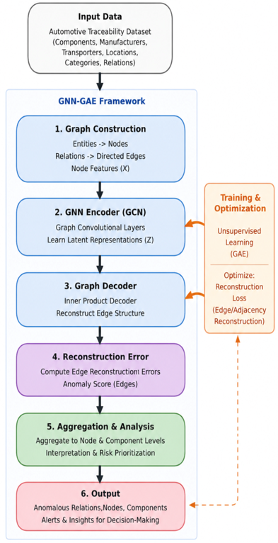
To take advantage of the inter-relationships among the different types of entities involved in the automotive supply chain, this study develops a framework for identifying anomalies using GNNs and GAEs. This is in contrast to the typical tabular approach that analyzes each component separately; since the traceability system can be represented as a relational graph, it provides the capability to simultaneously model the attributes of all entities as well as their respective relationships. Figure 1 presents the global architecture of the proposed GNN-GAE framework, from graph construction to the aggregation and interpretation of the anomaly scores.
Figure 1. Global architecture of the GNN-GAE framework
3.1 Designing the traceability graph
The original dataset contains automotive parts with attributes describing manufacture, transport, location, inspections, and quality control. To capture the interactions among all the entities involved in traceability, this tabular data is converted into an attributed graph defined by
$G=(V, E, X)$ (1)
where,
V: set of vertices.
E: relationship or edge between the vertices.
X: node feature matrix.
Each automotive part in the dataset is used as a vertex in this graph. Other traceability entities such as manufacturers, transporters, locations, and part types are also modelled as separate vertices. The relationships observed in the industrial traceability data are then turned into edges between the respective entities, so they can be traced through the entire supply chain [29].
The original traceability dataset contains 1000 automotive components described by manufacturing, logistics, location, inspection, and quality-related attributes. To represent this information as a relational system, each component was first modeled as a node. Additional nodes were then created for the distinct manufacturers, transporters, logistics locations, and component categories appearing in the dataset. This transformation produced an attributed heterogeneous graph composed of 1048 nodes, as detailed in Table 2.
Table 2. Composition of the attributed traceability graph
|
Node Category |
Meaning |
Number of Nodes |
|
Automotive components |
Individual components in the dataset |
1000 |
|
Manufacturers |
Distinct manufacturers represented as traceability entities |
16 |
|
Transporters |
Distinct transport and logistics actors |
11 |
|
Logistics locations |
Distinct previous and current locations appearing in the dataset |
5 |
|
Component categories |
Distinct component types or technical families |
16 |
|
Total |
All graph nodes |
1048 |
3.2 Node categories and relationship types
The created graph has been built with five classes (categories) for entities: Automotive Components; Manufacturers; Transporters; Logistics Locations; Component Categories. Each class contains all of the Nodes that have the same operational and semantic value or meaning in relation to the Traceability System. Relationships between entities are represented by five types of relationships found in the data set, these include Manufacturing Relationships; Transportation Relationships; Categorization Relationships; Current-Location Relationships; Logistics Transition Relationships.
These relationships illustrate how the various entities in the automotive supply chain interact with one another and their interdependencies.
A relationship between two nodes vi and vj is formally defined as follows:
$e_{i j}=\left(v_i, v_j\right)$ (2)
In order to allow information to be propagated across the network via edges, an inverse was assigned to every edge, therefore creating a Bidirectional Directed Graph. This will enable the model to leverage neighborhood information.
Transition relationships and current-location relationships are distinguished by their temporal meaning. A transition relationship represents a historical movement or passage recorded during the lifecycle of a component, whereas a current-location relationship represents the last known location of the component at the time of data extraction. Therefore, transition edges capture lifecycle movement history, while current-location edges capture the current operational state.
To provide a clear overview of the graph construction, the five relationship types—along with their respective source fields, directions, operational meanings, and edge counts—are comprehensively summarized in Table 3.
Table 3. Edge types used in the traceability graph
|
Edge Type |
Source Field in Raw Data |
Direction Before Adding Inverse Edge |
Operational Meaning |
Number of Original Edges |
|
Manufacturing relationship |
Manufacturer |
Component to Manufacturer |
Identifies the manufacturer responsible for the component |
1000 |
|
Transportation relationship |
Transporter |
Component to Transporter |
Identifies the transport or logistics actor associated with the component |
1000 |
|
Categorization relationship |
Component Type |
Component to Component category |
Links a component to its technical family or component type |
1000 |
|
Transition relationship |
Previous Location and Current Location |
Previous Location to Current Location |
Represents a historical movement or passage between two logistics locations during the component lifecycle |
20 |
|
Current-location relationship |
Current Location |
Component to Current Location |
Represents the last known location of the component at the time of data extraction |
1000 |
|
Total |
- |
- |
All original directed relationships before adding inverse edges |
4020 |
3.3 Node feature engineering
In the implemented model, the node feature matrix X includes node-type indicators, normalized numerical and temporal attributes, encoded quality and inspection indicators, and normalized degree features. Health status and inspection outcome were encoded as numerical attributes and included in X because they describe the operational condition of the components within the traceability system. Specifically, health status was encoded as Good = 0, Requires Inspection = 0.5, and Defective = 1, while Inspection Outcome was encoded as Passed = 0, Minor Issue = 0.5, and Failed = 1. Therefore, the subsequent analysis of anomaly scores according to health status and inspection outcome should be interpreted as a post-hoc consistency analysis rather than as an independent external validation. This analysis examines whether the high-priority components identified by the GAE are consistent with operational quality indicators already present in the traceability dataset.
Every single node has been assigned a feature vector:
$x_i=\left[x_{i 1}, x_{i 2}, \ldots, x_{i d}\right]$ (3)
This was done where 'd' represents the dimensionality of the feature space. This feature-construction strategy reflects the objective of modeling the traceability system as an attributed graph in which both relational structure and operational component attributes contribute to anomaly scoring. To avoid overstating the evaluation, health status and inspection outcome are not treated as independent ground-truth labels. They are used only after score computation to interpret the operational profile of high-priority components.
All the node feature vectors combine into one big attribute matrix:
$X \in \mathbb{R}^{N \times d}$ (4)
N- the total number of nodes in the graph.
This encoding strategy uses both relational structure and operational component attributes in the feature matrix. Because health status and inspection outcome are included in X, the subsequent comparisons with these variables are interpreted only as post-hoc consistency analyses, not as independent external validation or supervised performance evaluation.
3.4 Graph autoencoder architecture
We propose a GAE that utilizes a GCN. It learns a latent representation for every single node. This is done using both the node's own feature attributes and its neighboring nodes [30].
A GCN Layer Propagation Rule is defined as:
$H^{(l+1)}=\sigma\left(\widehat{D}^{-1 / 2} \hat{A} \widehat{D}^{-1 / 2} H^{(l)} w^l\right)$ (5)
where,
A: is the augmented adjacency matrix.
D: is the corresponding degree matrix.
$w^l$: is the trainable weights of layer l.
σ(.): denotes the activation function.
After several layers of graph convolution, we get our latent node representations:
$Z=\left[z_1, z_2, \ldots, z_N\right]$ (6)
Our decoder reconstructs graph connections from latent embeddings according to:
$\hat{A}=\sigma\left(Z Z^T\right)$ (7)
Our model is training by minimizing reconstruction error between original graph structure and reconstructed adjacency matrix. In our model, the encoder consists of two GCN layers. The first layer maps the input feature dimension d to 32 hidden units, followed by a rectified linear unit (ReLU) activation. The second layer maps the hidden representation to a latent embedding of dimension 16. The decoder reconstructs graph connectivity using an inner-product decoder followed by a sigmoid function. The model was trained for 200 epochs using the Adam optimizer, with a learning rate of 0.01 and a weight decay coefficient of 1 × 10⁻⁵.
3.5 Edge, node, and component anomaly scoring
If our GAE does not correctly reproduce normal relationship within the graph, then it will create anomalies with higher reconstruction errors [25].
We compute anomaly scores for edges:
$S_{\text {edge}}(i, j)=\left|A_{i j}-\hat{A}_{i j}\right|$ (8)
We compute anomaly scores for nodes by taking averages of incident edge anomaly scores:
$S_{\text {node}}(i)=\frac{1}{|N(i)|} \sum_{j \in N(i)} S_{\text {edge}}(i, j)$ (9)
N(i): the set of neighbors of node i.
We compute anomaly scores for components by aggregating all node anomaly scores:
$S_{\text {component}}=f\left(S_{\text {node}}\right)$ (10)
The component that has the largest anomaly score will need additional investigation.
3.6 Algorithm of the proposed framework
The complete computational procedure is summarized in Algorithm 1. Compared with the previous conceptual workflow, the revised algorithm specifies the graph construction, feature matrix construction, model architecture, training hyperparameters, negative sampling strategy, and anomaly-score computation rules.
|
Algorithm 1: Relational anomaly detection using the proposed GNN-GAE framework |
|
Input:
Output:
1: Extract component, manufacturer, transporter, component-type, and location entities from D. 2: Construct the heterogeneous node set V and the original edge set E using manufacturing, transportation, categorization, current-location, and transition relationships. 3: Aggregate duplicate relations and add inverse edges to obtain a bidirectional directed graph G = (V, E). 4: Build the node feature matrix X using node-type indicators, normalized numerical and temporal attributes, encoded quality and inspection indicators, and normalized degree features. 5: Initialize a two-layer GCN encoder with 18 input features, 32 hidden units, and 16 latent dimensions. 6: Initialize the GAE with the graph convolutional encoder and an inner-product decoder. 7: Train the model for 200 epochs using Adam with learning rate 0.01 and weight decay 1 × 10⁻⁵. At each epoch, sample negative edges with the same number as the observed positive edges. 8: After training, compute the final node embeddings Z. 9: Reconstruct the adjacency matrix using the inner-product decoder: Â = σ(ZZT) 10: For each observed edge eij ∈ E, compute the edge anomaly score according to Eq. (8): Sedge(i, j) = |Aij − Âij| 11: Since only observed traceability relations are scored, Aij = 1; therefore, the edge score is equivalent to: Sedge(i, j) = 1 − σ(ziTzj) 12: For each node vi, compute the node anomaly score as the mean anomaly score of its incident edges according to Eq. (9): Snode(i) = (1 / |N(i)|) Σj ∈ N(i) Sedge(i, j) 13: For each automotive component ck, compute the component anomaly score according to Eq. (10): Scomponent(k) = f(Snode) 14: Rank all automotive components in descending order of Scomponent(k). 15: Return the ranked list R and the corresponding edge, node, and component anomaly scores. |
In this algorithm, the general edge-score formulation |Aij − Âij| is consistent with the implementation because anomaly scores are computed for observed traceability relations. For such relations, Aij = 1 and Âij = σ(ziTzj), so the edge anomaly score is equivalent to 1 − σ(ziTzj). The component-level score is then obtained from the node-level anomaly scores according to the aggregation rule defined in Eq. (10).
4.1 Threshold definition and score statistics
To avoid interpreting small numerical differences as meaningful anomalies, high-priority components were defined using a percentile-based threshold. Specifically, components with anomaly scores greater than or equal to the 95th percentile of the component-score distribution were considered high-priority cases for operational investigation. This threshold does not imply confirmed failure; rather, it identifies the most atypical 5% of components according to the relational reconstruction score learned by the GAE. The same descriptive statistics were also computed at the edge and node levels to support a clearer interpretation of the score distributions.
As shown in Table 4, the maximum values alone are not sufficient to define anomalous behavior, because reconstruction scores are relative indicators rather than direct labels of operational failure. For this reason, the 95th percentile threshold was used to identify the components that deviate most strongly from the dominant relational patterns in the traceability graph. These high-priority components were then analyzed according to their component type, manufacturer, transporter, current location, health status, and inspection outcome.
To complement the analysis of anomaly-score distributions, an additional methodological comparison was conducted to clarify the role of relational graph modeling in the proposed framework. Because manually verified anomaly labels are not available, the comparison is interpreted as a ranking-oriented analysis rather than as supervised classification performance. Table 5 summarizes the role of tabular baselines, feature-only ablation, and hyperparameter-sensitivity considerations in the interpretation of the proposed GAE results.
Table 5 shows that tabular baselines and the feature-only ablation analyze component attributes independently, while the proposed GAE also models traceability relationships. This relational modeling capacity is important because atypical manufacturer, transporter, category, transition, or location links may reveal inconsistencies that are not visible from attributes alone. The sensitivity considerations further support interpreting the output as a ranking of high-priority cases for operational investigation rather than as binary anomaly labels.
Table 4. Descriptive statistics of anomaly scores at different analysis levels
|
Score Level |
Mean |
Standard Deviation |
Minimum |
95th Percentile |
Maximum |
|
Edge score |
0.086219 |
0.042401 |
0.000000 |
0.146515 |
0.195603 |
|
Node score |
0.087462 |
0.013966 |
0.023875 |
0.109046 |
0.169494 |
|
Component score |
0.086651 |
0.011387 |
0.054088 |
0.104868 |
0.127839 |
Table 5. Summary of baseline, ablation, and sensitivity considerations
|
Analysis Item |
Compared or Varied Element |
Purpose |
Interpretation |
|
Tabular baseline comparison |
Principal component analysis (PCA), isolation forest, local outlier factor |
Compare the proposed graph-based ranking with common attribute-based anomaly detection methods |
Tabular methods identify abnormal components from attributes only and do not model traceability relations |
|
Feature-only ablation |
Feature-only autoencoder without graph connectivity |
Assess the role of relational structure |
Removing graph connectivity prevents the detection of atypical manufacturer, transporter, location, and transition relationships |
|
Hyperparameter sensitivity |
Hidden dimension, latent dimension, learning rate, number of graph convolutional layers |
Assess the stability of the anomaly ranking |
Stable high-priority components indicate that the ranking is not caused by a single arbitrary configuration |
|
Proposed framework |
Attributed traceability graph with graph convolutional encoder and inner-product decoder |
Combine component attributes and relational structure |
Produces edge, node, and component anomaly scores for operational prioritization |
4.2 Overall distribution of anomaly scores
The GAE model generates an anomaly score for each relationship in the graph according to its reconstruction error.
Figure 2 illustrates the distribution of anomaly scores calculated for all relationships contained in the traceability network.
Figure 2. Overall distribution of the relation anomaly scores
All relationships have very low reconstruction-error values, which indicates that the GAE has successfully captured the predominant structural features of the traceability system. However, there are some relationships (relatively few) with much larger reconstruction-error values than those obtained by the other relationships, corresponding to abnormal interactions, outside the relational patterns learned by the model during training. The asymmetry observed is typical of anomaly-detection systems; abnormal conditions occur relatively infrequently.
4.3 Analysis of critical relationships and nodes
The analysis of reconstruction errors allows us to identify which relationships within the traceability network are the most atypical. The largest anomaly-scores are primarily associated with interactions involving certain manufacturers, components and transporters. Some of the most important relationships include links connecting components to manufacturers like Varta and Robert Bosch GmbH. These linkages show reconstruction errors that greatly exceed the average reconstruction error for the entire traceability network, therefore, they are far out of line with the dominant relational patterns learned by the model. The fact that these deviations from relational patterns could be caused by rare or previously unseen logistical arrangements, atypical location changes, unusual behavior of particular supply-chain participants or possible increased traceability risk can be investigated using aggregation of edge-anomaly-scores into node-anomaly scores, to find entities which frequently interact in irregular ways [16, 31, 32].
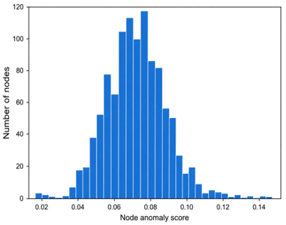
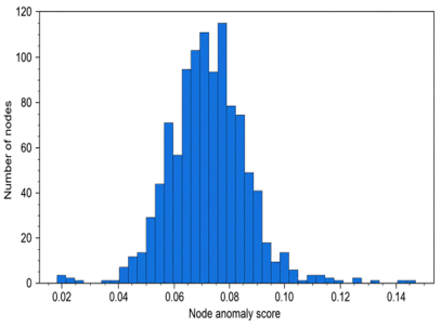
The distributions of node-anomaly scores shown in Figure 3 illustrate that most entities are clustered about mid-score values while a smaller number of nodes were found to be highly anomalous, because they are involved in atypical relational configurations.
Figure 3. Distribution of node anomaly scores
A deeper investigation into the most critical nodes showed that many manufacturers had high anomaly scores, i.e., Varta, Robert Bosch GmbH, Samsung SDI and Magna International. Additionally, there was evidence of a greater than average anomaly level of certain component types such as voltage converters, cooling systems, processors, and cameras. Since both the manufacturer and component type appeared together in the list of top 5 critical nodes it would appear that this anomaly was due to complex relational patterns rather than just the properties of a single entity. The results of our research demonstrate how valuable graph models can be for analyzing industrial traceability systems. As opposed to traditional methods, the proposed method did not only detect anomalous parts but also identified the components and relationships that contributed most to structural anomalies present throughout a supply chain.
4.4 Classification of abnormal components
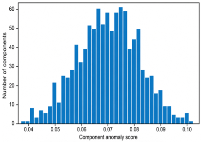
Node-level anomaly scores are subsequently aggregated to compute a global anomaly score for each automotive component, whose distribution is shown in Figure 4.
Figure 4. Distribution of component anomaly scores
By aggregating the data (i.e., by moving away from a relational view to one based on business needs), the analysis now supports the needs of both quality and logistics departments. The component level analysis will also indicate that most of the automotive parts which have the highest anomaly scores, cluster together and are therefore concentrated in a small number of automotive components; e.g. CMP-0310, CMP-0920, CMP-0936, CMP-0160, CMP-0744, CMP-0073, CMP-0207, CMP-0361, CMP-0816, and CMP-0902. These automotive components display relational patterns that differ significantly from those patterns displayed by the majority of automotive components in the traceability network. It indicates there may be some traceability inconsistencies, atypical logistics processes, or relationships with other entities within the network that are out of the norm. Identifying these automotive components will assist quality professionals with identifying the best candidates for pro-active monitoring and thus allow them to focus their efforts on those parts that represent the greatest risk regarding either quality, compliance or logistics performance. Additionally, this demonstrates how the use of the proposed framework has allowed for the conversion of relational anomalies into actionable indicators for component level decisions that can help facilitate decision making processes in complex industrial traceability networks [16, 33].
4.5 Post-hoc consistency analysis based on health status and inspection results
4.5.1 Analysis by health status
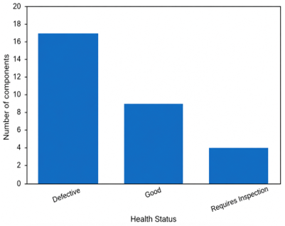
As shown in Figure 5, it appears that a higher proportion of high-priority components were located on components whose overall health was classified as being in poor shape.
This result shows that the high-priority components identified by the GAE are consistent with unfavorable operational indicators. However, because health Status is included in the node feature matrix, this analysis should not be interpreted as independent validation or proof of operational failure. It is used as a post-hoc consistency check to support the operational interpretation of the anomaly ranking.
Figure 5. Distribution of anomalies by component health status
4.5.2 Analysis based on inspection outcome
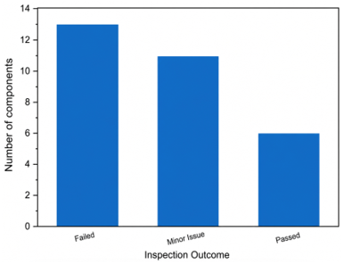
A similar relationship exists in the inspection results, as shown in Figure 6. Those components inspected and found to contain defects had higher defect scores than those components that passed all quality control tests.
Figure 6. Breakdown of anomalies by inspection results
Because no manually verified ground-truth anomaly labels exist for this dataset, the comparison with Inspection Outcome is not used as an independent validation measure. Since inspection information is included in the feature matrix, this analysis is interpreted as a post-hoc consistency check showing how the highest-ranked components relate to operational quality outcomes.
4.6 Analysis by component type, manufacturer, carrier, and location
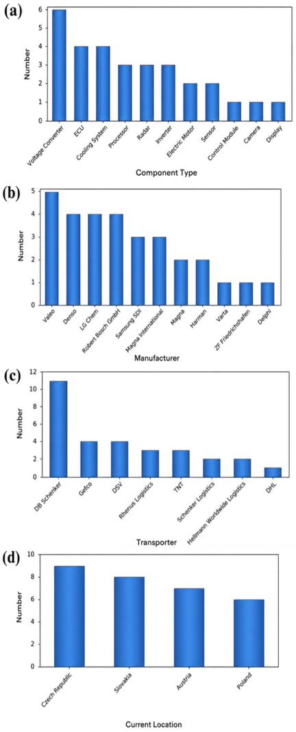
To further understand the detected anomalies, an additional investigation has been performed based on the major entities in the traceability system which include component types, manufacturers, carriers, and locations. An additional investigation was performed to determine the categories that were most commonly associated with components having high anomaly scores. Figure 7 shows the distribution of the anomalous components according to (a) component type, (b) manufacturer, (c) transporter, and (d) current location.
Figure 7. Distribution of anomalous components according to (a) component type, (b) manufacturer, (c) transporter, and (d) current location
These entity-level concentrations should be interpreted as prioritization signals for further investigation rather than as confirmed causal explanations.
The results show that certain categories of components are more common among the most important components, therefore they could be more susceptible to logistics disruptions or inconsistencies in traceability. In addition, there is evidence that several of the suppliers had a disproportionate number of anomalous components, thus providing some indication of the level of risk for each supplier and also an opportunity to investigate issues related to quality. Furthermore, it appears that specific transporters appeared to have multiple instances of anomalous components and possibly even more than one instance of the same anomalous component. Therefore, this would suggest that specific transportations processes and/or routes may require additional oversight. Also, the location analysis demonstrates that specific logistics locations have occurred in the traceability paths of anomalous components; therefore, they can represent potentially critical points in the logistics network.
These findings provide clear evidence that the anomalies found using the proposed method are not evenly distributed throughout the traceability network, but rather cluster around specific types of entities. Thus, the ability to localize potential risk areas is beneficial for proactive monitoring, targeted corrective action and continued supply chain performance.
4.7 Latent space analysis
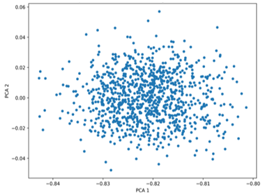
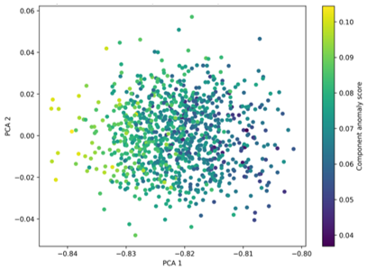
One of the primary advantages of the GAE is its ability to create a latent representation of the graph [34]. To analyze this representation, the learned node embeddings are projected into two dimensions using PCA. Figure 8 shows the resulting projection of the component embeddings, while Figure 9 shows the same projection with the points colored according to their anomaly scores.
Figure 8. Two-dimensional PCA projection of the component embeddings
Figure 9. Two-dimensional PCA projection of component embeddings, colored according to their anomaly scores
This projection provides a visual interpretation of the latent space learned by the model and highlights how the components are structured in the learned representation space.
This anomaly-colored projection demonstrated that there are unique groups of entities that share common relational properties. The entities determined to be anomalous are mostly at the edge of the majority groupings or in a sparsely populated area in the latent space. This indicates that structural patterns exist that deviate from those observed throughout the entire traceability network. This is an indication that the proposed model appropriately identifies significant relational patterns and can differentiate unusual behavior from regular operating behaviors by utilizing the learned latent representations for detecting anomalies in large industrial traceability networks.
Beginning with the issue of identifying inconsistencies in the traceability of automotive parts within supply chains through a relational representation of traceability data, the study provided a new way to represent traceability through the creation of a complex network of connected entities. Components, manufacturers, carriers, and storage facilities were all represented through multiple logistics connections. An unsupervised combination of GNNs and GAEs were used to find structural anomalies in a traceability network for automobiles. A traceability data set containing 1000 automobile components identified with 19 different features was converted into an attributed graph with 1048 nodes and 8040 directed edges. Using a GCN as part of the GAE architecture allowed the model to learn the underlying latent structures of the entities and create a reconstructed version of the input graph. Errors from the reconstruction process were then used to calculate anomaly scores for each relationship, node, and component. Experimental results show that the method is able to identify unusual interactions between certain manufacturers, component types, carriers, or storage facilities; in addition, many components exhibited significantly large inconsistencies in their structural integrity. The analysis using the health status and inspection outcome indicators provided further evidence that the identified anomalies have some level of industrial applicability. The results indicate that the methodology may support automotive traceability monitoring by prioritizing components and relationships that deviate from dominant relational patterns. Its transfer to other regulated industries, such as aerospace or pharmaceuticals, would require additional validation on domain-specific datasets. Tabular methodologies traditionally assess the properties of components individually. However, the methodology also considers both the properties of components as well as the relational dependencies between them in order to assess traceability risks comprehensively. It can also provide a means to discover inconsistencies that would likely be undetectable through traditional methodologies. Additionally, there are several practical applications for the methodology. These include proactively monitoring traceability-related issues, improving product quality, managing supplier risk, and providing decision-making support in complex industrial settings. However, there are several limitations to acknowledge regarding the findings. Because no ground-truth anomaly labels were available, the evaluation relies on indirect validation against business indicators rather than on supervised metrics such as precision, recall, or AUC. Because no manually verified anomaly labels were available, the evaluation relied on proxy operational indicators and ranking-based interpretation rather than supervised metrics such as precision, recall, or AUC. The comparison with tabular baselines and the feature-only ablation was therefore used to clarify the methodological contribution of relational graph modeling, while future work should extend this evaluation using labelled traceability incidents. Another limitation is that the validation relies on proxy operational indicators rather than manually verified anomaly labels. Future work should use labelled traceability incidents, larger multi-company datasets, and controlled comparisons with additional graph anomaly detection methods. The methodology is also dependent upon static data and a single example case from the automotive industry. Furthermore, although it assesses the graph structure of traceability data, it does not directly take into account the time-based nature of traceability events. Therefore, future work could involve assessing whether dynamic versions of GNNs (e.g., DGNNs), attention-based architectures (e.g., Graph Transformers), or real-time IoT data will increase early detection capabilities for anomalies. Another possible avenue for investigation includes comparing this methodology to state-of-the-art GRL architectures and assessing how applicable they are across various industrial domains (aerospace, pharmaceutical manufacturing, multimodal transportation networks).
The authors would like to express their sincere gratitude to the Laboratory of Modeling and Simulation of Intelligent Industrial Systems (M2S2I) for providing the scientific environment and research support that contributed to the completion of this work. The authors also acknowledge the École Normale Supérieure de l’Enseignement Technique (ENSET Mohammedia) and Hassan II University of Casablanca for their academic support and for fostering a stimulating research environment that facilitated the development of this study.
|
A |
adjacency matrix, dimensionless |
|
 |
reconstructed adjacency matrix, dimensionless |
|
D |
degree matrix, dimensionless |
|
E |
set of edges, dimensionless |
|
G |
attributed graph, dimensionless |
|
N(i) |
set of neighboring nodes of node i, dimensionless |
|
Sedge |
edge-level anomaly score, dimensionless |
|
Snode |
node-level anomaly score, dimensionless |
|
Scomponent |
component-level anomaly score, dimensionless |
|
V |
set of vertices, dimensionless |
|
X |
node feature matrix, dimensionless after encoding/normalization |
|
xi |
feature vector of node i, dimensionless |
|
Z |
latent embedding matrix, dimensionless |
|
zi |
latent representation of node i, dimensionless |
|
σ |
activation function |
|
W(l) |
trainable weight matrix at layer l |
[1] Miehle, D., Henze, D., Seitz, A., Luckow, A., Bruegge, B. (2019). PartChain: A decentralized traceability application for multi-tier supply chain networks in the automotive industry. In 2019 IEEE International Conference on Decentralized Applications and Infrastructures (DAPPCON), Newark, CA, USA, pp. 140-145. https://doi.org/10.1109/DAPPCON.2019.00027
[2] Paolucci, E., Pessot, E., Ricci, R. (2021). The interplay between digital transformation and governance mechanisms in supply chains: Evidence from the Italian automotive industry. International Journal of Operations & Production Management, 41(7): 1119-1144. https://doi.org/10.1108/ijopm-09-2020-0672
[3] Khan, M., Parvaiz, G.S., Dedahanov, A.T., Abdurazzakov, O.S., Rakhmonov, D.A. (2022). The impact of technologies of traceability and transparency in supply chains. Sustainability, 14(24): 16336. https://doi.org/10.3390/su142416336
[4] Abbad, H., Souak, S., Mahjoub, S. (2025). Internet des objets, blockchain et big data: Quel(s) rôle(s) pour la prise de décision dans la supply chain automobile? Revue Française de Gestion Industrielle, 39(1): 29-41. https://doi.org/10.53102/2025.39.01.1183
[5] Ahmed, W.A., MacCarthy, B.L. (2023). Blockchain-enabled supply chain traceability-How wide? How deep? International Journal of Production Economics, 263: 108963. https://doi.org/10.1016/j.ijpe.2023.108963
[6] McKEAN, J.D. (2001). The importance of traceability for public health and consumer protection. Scientific & Technical Review, 20(2): 363-371. https://doi.org/10.20506/rst.20.2.1280
[7] Kirov, A. (2020). Traceability system as a component of lifecycle management of radio-electronic products. International Journal of Innovative Technology and Exploring Engineering, 4(9): 3251-3254. https://doi.org/10.35940/ijitee.d1942.029420
[8] Campos, J.G., Miguez, L.R. (2009). Manufacturing traceability data management in the supply chain. International Journal of Information Technology and Management, 8(3): 321. https://doi.org/10.1504/ijitm.2009.024608
[9] Robson, C., Watanabe, Y., Numao, M. (2006). Parts traceability for manufacturers. In 2007 IEEE 23rd International Conference on Data Engineering, Istanbul, Turkey, pp. 1212-1221. https://doi.org/10.1109/ICDE.2007.368980
[10] Zanibbi, R., Blostein, D., Cordy, J.R. (2004). A survey of table recognition. International Journal on Document Analysis and Recognition, 7(1): 1-16. https://doi.org/10.1007/s10032-004-0120-9
[11] Ghodake, S.P., Malkar, V.R., Santosh, K., Jabasheela, L., Abdufattokhov, S., Gopi, A. (2024). Enhancing supply chain management efficiency: A data-driven approach using predictive analytics and machine learning algorithms. International Journal of Advanced Computer Science and Applications, 15(4): 672-686. https://doi.org/10.14569/ijacsa.2024.0150469
[12] Meshram, A., Karch, M., Haas, C., Beyerer, J. (2025). Towards graph-based self-learning of industrial process behaviour for anomaly detection. Procedia Computer Science, 270: 3913-3923. https://doi.org/10.1016/j.procs.2025.09.516
[13] Zhang, C., Jeong, J., Jung, J. (2025). Anomaly detection over multi-relational graphs using graph structure learning and multi-scale meta-path graph aggregation. IEEE Access, 13: 60303-60316. https://doi.org/10.1109/access.2025.3554407
[14] Kim, H., Lee, B.S., Shin, W., Lim, S. (2022). Graph anomaly detection with graph neural networks: Current status and challenges. IEEE Access, 10: 111820-111829. https://doi.org/10.1109/access.2022.3211306
[15] Ahmed, I.A., Moghaddass, R. (2024). Anomaly detection in graph-based data utilizing graph topology. In 2024 Annual Reliability and Maintainability Symposium (RAMS), Albuquerque, NM, USA, pp. 1-6. https://doi.org/10.1109/RAMS51492.2024.10457635
[16] Guelail, R., Ennadafy, H., Belouaggadia, N. (2026). Unsupervised learning-based detection of traceability anomalies in automotive supply chains using isolation forest and reconstruction error-based principal component analysis. In 2026 6th International Conference on Innovative Research in Applied Science, Engineering and Technology (IRASET), FEZ, Morocco, pp. 1-9. https://doi.org/10.1109/IRASET68627.2026.11538524
[17] Ribeiro, D., Matos, L.M., Cortez, P., Moreira, G., Pilastri, A. (2021). A comparison of anomaly detection methods for industrial screw tightening. In International Conference on Computational Science and Its Applications, Cagliari, Italy, pp. 485-500. https://doi.org/10.1007/978-3-030-86960-1
[18] Shah, B.K., Lodhi, R.K., Tiwari, R.K. (2026). Anomaly detection in industrial machine time series data using machine learning technique. In 2026 6th International Conference on Pervasive Computing and Social Networking (ICPCSN), Salem, India, pp. 964-968. https://doi.org/10.1109/ICPCSN68523.2026.11543711
[19] Chliah, H., Battou, A., el Hadj, M.A., Laoufi, A. (2023). Hybrid machine learning-based approach for anomaly detection using Apache Spark. International Journal of Advanced Computer Science and Applications, 14(4): 870-878. https://doi.org/10.14569/ijacsa.2023.0140496
[20] Luo, Z., Dubey, R., Papadopoulos, T., Hazen, B., Roubaud, D. (2017). Explaining environmental sustainability in supply chains using graph theory. Computational Economics, 52(4): 1257-1275. https://doi.org/10.1007/s10614-017-9688-2
[21] Liu, J., Li, P., Wang, Y. (2026). Graph neural networks for modeling complex dependencies in global supply chain networks. Journal of Computing and Electronic Information Management, 20(3): 9-20. https://doi.org/10.54097/6fcw2b19
[22] Al Bataineh, A., Mairaj, A., Kaur, D. (2020). Autoencoder based Semi-Supervised Anomaly Detection in Turbofan Engines. International Journal of Advanced Computer Science and Applications, 11(11): 41-47. https://doi.org/10.14569/ijacsa.2020.0111105
[23] Bai, L., Cui, L., Hancock, E., Li, M., Wang, Y., Xu, Z. (2024). HC-GAE: The hierarchical cluster-based graph auto-encoder for graph representation learning. Advances in Neural Information Processing Systems, 37: 127968-127986.
[24] Roy, A., Shu, J., Li, J., et al. (2024). GAD-NR: Graph anomaly detection via neighborhood reconstruction. In WSDM '24: The 17th ACM International Conference on Web Search and Data Mining, Merida Mexico, pp. 576-585. https://doi.org/10.1145/3616855.3635767
[25] Kim, S., Lee, S.Y., Bu, F., et al. (2024). Rethinking reconstruction-based graph-level anomaly detection: Limitations and a simple remedy. Advances in Neural Information Processing Systems, 37: 95931-95962.
[26] Salha, G., Hennequin, R., Vazirgiannis, M. (2020). Simple and effective graph autoencoders with one-hop linear models. In Joint European Conference on Machine Learning and Knowledge Discovery in Databases, pp. 319-334. https://doi.org/10.1007/978-3-030-67658-2_19
[27] Duan, S., Ding, R., He, J., Ding, A., Fei, Y., Xu, X. (2024). GraphCroc: Cross-correlation autoencoder for graph structural reconstruction. Advances in Neural Information Processing Systems, 37: 45409-45437.
[28] Wu, X., Cheng, Q. (2022). Stabilizing and enhancing link prediction through deepened graph auto-encoders. In Thirty-First International Joint Conference on Artificial Intelligence IJCAI-22, Vienna, Austria, pp. 3587-s3593. https://doi.org/10.24963/ijcai.2022/498
[29] Kuhn, M., Franke, J. (2021). Data continuity and traceability in complex manufacturing systems: a graph-based modeling approach. International Journal of Computer Integrated Manufacturing, 34(5): 549-566. https://doi.org/10.1080/0951192x.2021.1901320
[30] Zhou, X., Wang, H., Li, Z., Zhang, S. (2020). Graph autoencoder combined with attribute information in graph. In 2020 6th International Conference on Big Data and Information Analytics (BigDIA), Shenzhen, China, pp. 28-34. https://doi.org/10.1109/BigDIA51454.2020.00014
[31] Han, H., Huang, D. (2025). Graph-theoretic detection of anomalies in supply chains: A PoR-based approach using Laplacian flow and sheaf theory. Mathematics, 13(11): 1795. https://doi.org/10.3390/math13111795
[32] Fessina, M., Zaccaria, A., Cimini, G., Squartini, T. (2024). Pattern-detection in the global automotive industry: A manufacturer-supplier-product network analysis. Chaos, Solitons & Fractals, 181: 114630. https://doi.org/10.1016/j.chaos.2024.114630
[33] Kuhn, M., Funk, F., Franke, J. (2021). Blockchain architecture for automotive traceability. Procedia CIRP, 97: 390-395. https://doi.org/10.1016/j.procir.2020.05.256
[34] Park, J., Lee, M., Chang, H.J., Lee, K., Choi, J.Y. (2019). Symmetric graph convolutional autoencoder for unsupervised graph representation learning. In 2019 IEEE/CVF International Conference on Computer Vision (ICCV), Seoul, Korea (South), pp. 6518-6527. https://doi.org/10.1109/ICCV.2019.00662