
S.M. Baque Billah* | Mohammed Amran | Ahamed-Al Arifin | Mashky Chowdhury Surja
© 2026 The authors. This article is published by IIETA and is licensed under the CC BY 4.0 license (http://creativecommons.org/licenses/by/4.0/).
OPEN ACCESS
Nowadays, wind energy significantly contributes to the ongoing shift towards renewable energy sources. Nonetheless, low wind velocity is one of the climatic constraints that reduce the power generation capability of wind turbines. However, the INVELOX wind concentrator offers a sustainable alternative for deploying wind turbines in regions with low wind velocity. The performance of the INVELOX wind system is highly sensitive to key geometric parameters such as inlet height (IH), funnel diameter (FD), and venturi diameter (VD). To analyze the performance of the INVELOX system by optimizing these parameters typically requires computationally expensive computational fluid dynamics (CFD) simulations. These intensive CFD simulations limit rapid design iteration and location-specific calibration. To address these challenges, this research presents a validated MATLAB/Simulink -based surrogate model to efficiently predict the INVELOX speed ratio (SR). This model also resolves the limitations and flaws of the existing basic MATLAB model. The proposed model is developed using high-fidelity ANSYS Fluent simulation data, which is a function of IH, FD, VD, and inlet velocity. Through CFD analysis, relevant parametric datasets were generated and used to derive physics-informed analytical equations via regression, which were then integrated into a dynamic MATLAB/Simulink framework. This developed MATLAB model was validated against 250 additional CFD test cases, and the results demonstrate strong agreement with the benchmark results, with an average predictive accuracy exceeding 98%. The developed framework also reduces computational time from hours to seconds while maintaining high predictive reliability and enabling researchers or designers to rapidly optimize geometry to evaluate site-specific performance. Overall, the proposed MATLAB model will provide a scalable alternative to CFD-driven workflows and will accelerate the deployment of INVELOX-based wind energy systems in low- to moderate-wind regimes.
INVELOX, computational fluid dynamics, surrogate modelling, MATLAB/Simulink, speed ratio, parametric dataset, predictive accuracy, scalable alternative
The current state of the global climate is a significant concern worldwide. The operation of nuclear, steam, and gas turbine power plants is directly associated with increases in average global temperature. In many applications, renewable energy sources are demonstrating substantial environmental advantages with economic viability [1]. Renewable energy also play an essential complementary role for advancing the climate mitigation goals, escalating electricity access, reinforcing energy security and alleviating the detrimental impacts of fossil fuel dependency [2]. Due to renewability, scalability, and potential to drive national energy transitions, the wind energy stands out as one of the fastest-growing renewable resources [3]. The United Nations Sustainable Development Goal 7 is closely aligns with the outcome that wind energy provides, as it supports access to affordable, reliable and sustainable modern energy for all [4]. Windmills are ancient technology for harnessing wind energy and have been utilised for more than 3,000 years [5]. A recent report shows that the wind power ranks as the second-largest contributor to renewable electricity generation after hydropower [6]. In 2024, renewable energy sources contributed 33 exajoules (EJ) to global energy consumption, accounting for 8% of total energy consumption, with wind energy generation increasing by 11.1% (25% of renewable capacity) and achieving 1,133 GW of installed power [7, 8]. Projections indicate that global energy demand will rise by about 1% each year through 2030, and under the Stated Policies Scenario (STEPS), renewable energies are expected to satisfy nearly all incremental demand [9]. However, the economic and technical feasibility of wind projects is constrained by the site-specific geographical, infrastructural, and economic factors [10, 11].
Like other advanced wind turbine configurations, the INVELOX system accelerates the ambient airflow by using specially designed ducts with a converging funnel and a venturi segment. This unique method improves the energy conversion efficiency, especially at low wind speeds [12]. The omnidirectional air intake structure of the INVELOX further improves air capture and boosts the acceleration efficiency across various wind directions [13]. The performance of that system is optimized by varying the nozzle-diffuser geometry and adjusting the diffuser parameter in the Venturi section [14, 15]. On the other hand, the boosted air acceleration increases the air’s kinetic energy by approximately 20–30 kg·m²/s² and improves the low-wind operability [16]. However, the wind direction also has a considerable influence on INVELOX efficiency, which has been analyzed and optimized in the study [17]. In that article, two key principles were mentioned which could help to achieve a high level of efficiency. One principle is increasing the pressure drop in turbines, and the other one is increasing the mass flow rate of air [18]. A comprehensive quantitative evaluation was also done in the study [19] to identify the critical geometrical parameters that govern the aerodynamic behavior and performance of INVELOX.
Generally, the performance of the INVELOX system is measured in terms of speed ratio (SR). The SR is defined as the ratio of Venturi-section wind speed to ambient wind speed and is highly sensitive to geometric configuration Parameters of the INVELOX. Based on prior research, the key geometric parameters of the INVELOX system are the inlet height (IH), funnel diameter (FD), and venturi diameter (VD). The studies have also shown that minor adjustments of those key geometric parameters have a significant effect on flow acceleration and pressure. These findings underline the necessity for the site-specific and precise optimization of those parameters [17, 19, 20]. On the other hand, it is evident that modifying only two key geometric parameters at a time can improve SR from 1.6 to 2.4, while keeping the third parameter remains at its standard value [21, 22].
Conventionally, the analysis of INVELOX wind systems to resolve complex flow fields and to forecast system performance metrics has relied heavily on high-fidelity computational fluid dynamics (CFD) simulations, such as ANSYS Fluent [20]. The CFD simulation delivers exceptionally detailed and accurate results, but the computational intensity and execution time are high. This high computational intensity and execution time make CFD simulations impractical for the comprehensive exploration of multi-objective optimization [23]. Those limitations are potential barriers to essential rapid prototyping and early-stage design analysis of the INVELOX system. In recent years, surrogate and reduced-order modelling has become an effective approach to reduce the computational barrier of high-fidelity simulations in wind energy research. Such approaches substantially reduce computational requirements without sacrificing predictive reliability [24, 25]. Several studies have successfully developed Kriging, neural-network, and physics-informed surrogates for wind turbine performance prediction and design optimisation [26-29]. Following this trend, the present work develops a CFD-informed regression-based surrogate model specifically tailored for multi-parameter design of the INVELOX system.
Facilitating system-level modeling, efficient computation, and dynamic simulation and optimization, MATLAB/Simulink is used as an effective complementary platform. Due to its inherent flexibility and seamless coupling of electrical, mechanical, and fluid domains, Simulink is widely adopted for renewable energy system analysis [30]. In replacement of lengthy CFD workflows, Simulink-based models provide rapid, reliable performance predictions, facilitating early-stage design evaluation and iterative refinement [31]. To date, only one study has introduced an early-stage MATLAB/Simulink model for the INVELOX system for predicting the SR. That model permitted variation of only IH, which is a single geometric parameter, while the FD and VD were held fixed at reference values. Consequently, it could not support concurrent multi-parameter design exploration and site-specific geometry optimisation [32].
To overcome these limitations, this study has developed an improved comprehensive MATLAB/Simulink based analytical surrogate model of the INVELOX wind system using CFD-generated data for rapid prediction of SR across diverse operating regimes. Unlike existing approaches, the proposed MATLAB model allows researchers to make concurrent variation of two key geometric parameters, like IH and VD with FD held constant; IH and FD with VD fixed; lastly, VD and FD with IH fixed, which enables targeted optimisation of SR for location-specific conditions. Analytical equations describing these relationships were first established using vector-based geometric analysis and subsequently refined through regression-based coefficient calibration before being implemented within the MATLAB/Simulink environment.
The developed model has also been validated using the independent ANSYS Fluent simulation data. The Validation results demonstrate a strong concordance between the developed Simulink model predictions and the ANSYS CFD value of SR. The strong agreement with the benchmark results has also made this model a computationally efficient tool for preliminary analysis, sensitivity studies, and design modification. In low-to-moderate wind contexts, this proposed framework will provide a scalable resolution for modelling and optimising the INVELOX wind systems and other renewable energy technologies.
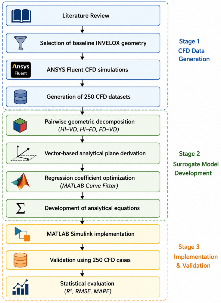
The overall research workflow is illustrated in Figure 1. The methodology integrates high-fidelity CFD simulations, analytical modelling, and system-level implementation to establish a computationally efficient surrogate model for predicting the SR under different geometric configurations. In this section, the MATLAB/Simulink model development for the INVELOX is thoroughly explained.
Initially, the original baseline INVELOX geometry model was selected from a detailed literature review. Then, the selected geometry was modeled in ANSYS Fluent to establish an ideal reference model for this article. After that the ANSYS reference model was used to investigate the impact of the critical geometric parameters, namely the IH, FD, and VD on the SR of INVELOX system. By altering those geometric configuration parameters, 250 characteristics datasets of INVELOX SR were generated through a large number of CFD simulations where the wind speed was considered as a location-specific constant speed. Unlike direct empirical curve fitting, the proposed modelling approach first analysed the CFD-generated datasets using vector-based analytical geometry to establish the dominant pairwise relationships between the governing geometric parameters and the corresponding SR. Three analytical models were therefore formulated for the geometric combinations IH–VD, IH–FD, and FD–VD, respectively. The analytical expressions obtained from the vector formulation were subsequently refined through regression-based coefficient calibration using MATLAB Curve Fitter to improve predictive accuracy while preserving the underlying analytical structure. The derived mathematical models were then implemented in MATLAB/Simulink environment to develop the proposed MATLAB model of INVELOX. This developed MATLAB model was then validated against the ANSYS reference model using 250 independent datasets to assess its effectiveness and accuracy compared to the ANSYS Fluent results using the statistical performance indicators, including the coefficient of determination (R²), root mean square error (RMSE), and percentage prediction accuracy.
Figure 1. Overall workflow of the proposed MATLAB/Simulink surrogate model development
2.1 INVELOX computational fluid dynamics model development and parametric dataset generation
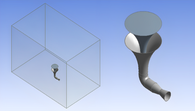
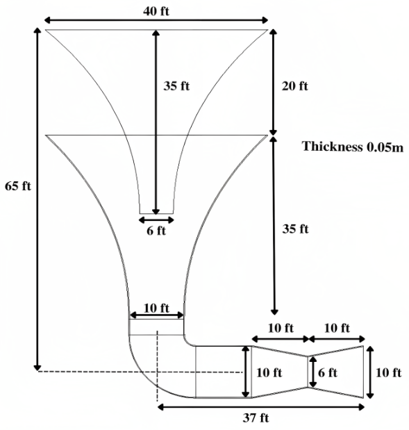
The INVELOX wind system was first proposed and analysed through CFD in the study [13]. The baseline geometric configuration parameters used in this research were adopted from that reference. Generally, the INVELOX system incorporates an inlet funnel, a Venturi contraction section, and a diffuser outlet. All those sections can be engineered to accelerate the incoming wind toward the turbine location. Based on the geometric dimensions mentioned in that reference study [13], the reconstructed ANSYS Fluent 3D model incorporates the following geometric dimensions: overall height of 65 ft, diffuser diameter of 10 ft, IH of 20 ft, FD of 40 ft, and VD of 6 ft. The INVELOX 3D structure with enclosure is illustrated in Figure 2, and the detailed geometric dimensions that are used in the simulation are presented in Figure 3.
Figure 2. Reconstructed 3D geometry of INVELOX in ANSYS
Figure 3. Schematic diagram of INVELOX with geometric dimensions
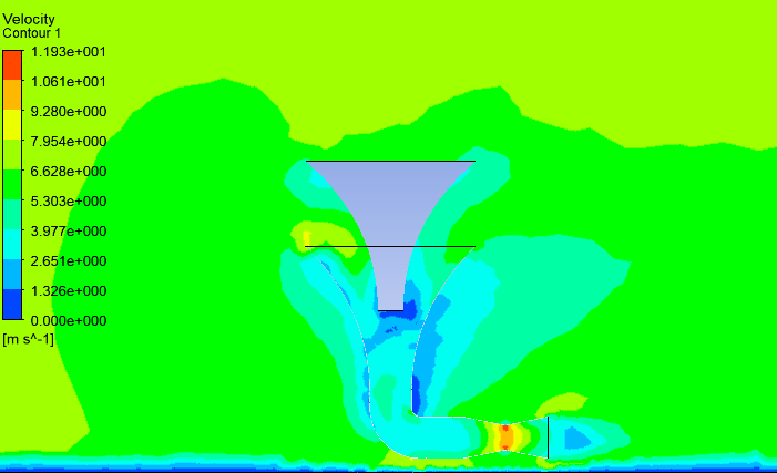
A validation simulation was also performed to verify the correctness of the reconstructed ANSYS models. During validation, the inlet wind speed and geometric parameters remain the same as in the reference study. The simulation results show that the SR = 1.58 is obtained at the venturi throat. The obtained SR value is consistent with the published reference study. This consistency confirms the reliability of the reconstructed CFD model. The corresponding velocity contour of the airflow inside the INVELOX venturi section is illustrated in the Figure 4.
Figure 4. Validation result of Allaei and Andreopoulos [13]
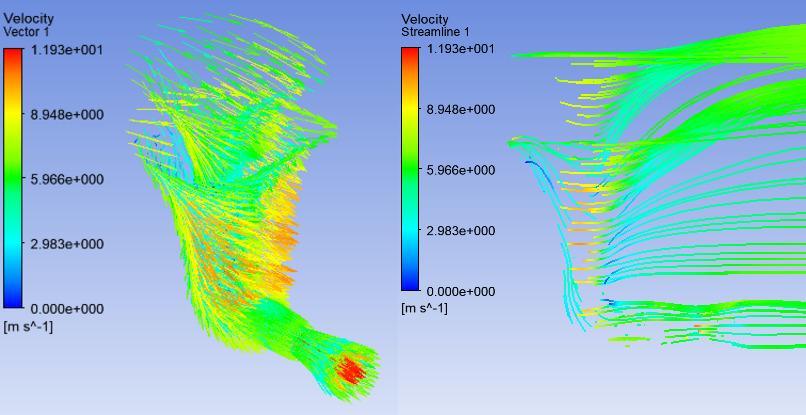
The CFD simulations were performed in ANSYS Fluent using a three-dimensional, steady-state, pressure-based solver. The computational mesh was generated using ANSYS Meshing. This process produces high-quality meshes that efficiently yield accurate CFD solutions [33]. Also, this process minimizes unnecessary numerical iterations during simulation in complex flow domains [34]. The used mesh size range was from 120,000 to 3,680,000 elements. To accurately capture the strong velocity gradients, local refinement was also applied near the Venturi throat. A mesh independence analysis was also performed, where the error in the estimated velocity at the Venturi throat was determined to be negligible beyond the selected mesh density. Velocity vector and velocity streamline of the reconstructed INVELOX CFD model are visible in Figure 5.
Figure 5. Velocity vector and streamline of result in developed ANSYS model of INVELOX
For turbulence model, the standard k–ε viscous turbulence model with standard wall functions was used as it is widely used in internal flow simulations due to its computational efficiency and robustness [35]. At the upstream face, velocity inlet boundary conditions were specified, while pressure-outlet conditions were imposed at the downstream and side faces. The ground and outer surfaces of the INVELOX structure were modelled as no-slip walls. Second-order upwind discretisation was employed for both momentum and turbulence variables. The SIMPLE algorithm was utilised for pressure–velocity coupling. Under-relaxation factors were maintained at the default values provided by Fluent. Convergence was achieved when the scaled residuals of continuity, momentum, and turbulence equations dropped below 10⁻⁵, and the monitored velocity at the Venturi throat reached a steady value.
To generate the datasets for the mathematical model, three groups of parametric simulations were conducted, which captured the influence of three key geometric parameters of INVELOX on SR value. The three key geometric parameters considered were: IH, VD, and FD, because they have been consistently reported as the key geometric variables governing wind acceleration, pressure distribution, and the resulting SR [17, 19, 20]. Conducted parametric simulations were based on the IH–VD, IH–FD, and FD–VD geometric configurations, where two parameters were varied for each configuration. In contrast, the third parameter was maintained at a constant reference value.
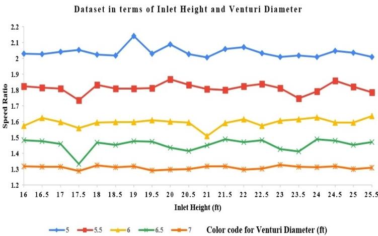
The first group of simulations was conducted based on the IH-VD configuration, where the IH and VD were varied while keeping the FD constant at baseline optimal value. Here, the IH varies from 16 ft to 25.5 ft and the VD from 5 ft to 7 ft, while the FD remains constant at 40 ft. This configuration produced a first dataset of 100 simulation data points. The resulting SR dataset is illustrated in Figure 6.
Figure 6. A dataset of SR was produced through 100 simulation runs concerning the IH-VD configuration, demonstrating the impact of changing IHs (ranging from 16 to 25.5 ft) and VDs (from 5 to 7 ft) while maintaining a constant FD of 40 ft
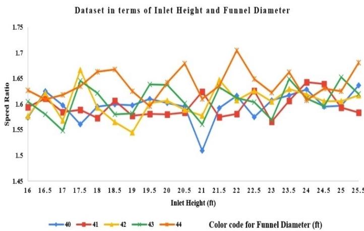
To create a second dataset for this study, a second group of simulations were conducted based on the IH-FD configuration. In this configuration, the IH and FD varied while the VD remained fixed at the baseline optimal value. During simulation, the IH varies between 16 ft and 25.5 ft, and the FD between 40 ft and 44 ft, while maintaining the VD constant at 6 ft. This configuration generated 100 simulation data samples for the second dataset. The resulting SR dataset of IH-FD configuration is presented in Figure 7.
Figure 7. A dataset on SR was created through 100 simulation runs for the IH-FD setup, demonstrating the impact of changing IHs (16–25.5 ft) and FDs (40–44 ft) while maintaining a consistent VD of 6 ft
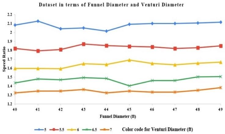
Finally, the third group of simulations were conducted based on the FD–VD configuration where the FD and VD were varied, while the IH was kept at the baseline optimal value. Here the FD varies from 40 ft to 49 ft and the VD from 5 ft to 7 ft, while the IH remains constant at 20 ft. This configuration produced a third dataset of 50 simulation data points. Figure 8 shows the resulting SR dataset.
The ranges IH = 16–25.5 ft, FD = 40–49 ft, and VD = 5–7 ft were selected to capture practical variations relative to the baseline geometry established in [13]. These ranges provide sufficient variation for constructing accurate surrogate models applicable to location-specific geometric optimisation, while remaining within the structural and manufacturing constraints reported in subsequent INVELOX studies [17, 19-22]. From those three groups, total 250 CFD simulation data samples were collected. For each simulation, an inlet wind velocity of 5.37 ms⁻¹ was applied. This wind velocity corresponds to the average wind speed in Chattogram as reported by the Bangladesh Meteorological Department (BMD) [36]. It should be noted that all CFD simulations were performed at a single inlet velocity of 5.37 m/s, which is in the range of low-to-moderate wind speeds. Therefore, the current surrogate model is calibrated for a low-to-moderate wind regime. The airflow velocity at the venturi throat was extracted from the simulation results and used to calculate the corresponding SR. Those CFD analytical datasets serve as the foundation for the mathematical model development. A separate set of 250 CFD simulations, generated with varied geometric combinations within the same parameter ranges, was subsequently utilised to validate the developed MATLAB/Simulink framework.
Figure 8. The SR dataset was produced through 50 simulation trials for the FD–VD setup, demonstrating the impact of changing FDs (ranging from 40 to 49 ft) and VDs (from 5 to 7 ft), all while maintaining a constant IH of 20 ft
2.2 Mathematical model development
The proposed methodology develops the mathematical model from the CFD analytical data by integrating vector-based analytical geometry with regression-based coefficient optimisation, rather than relying solely on empirical regression models. This method preserves the dominant geometric relationships identified in the CFD-generated datasets and improves predictive accuracy. To examine the relationship between geometric parameters and the corresponding SR, the CFD dataset was initially visualised using MATLAB 3D surface plots. These surfaces exhibited an irregular planar trend, indicating that the primary trend could be represented by an analytical plane. Four representative boundary points from each parametric domain were selected to construct an initial analytical plane using vector geometry. The cross product of two independent vectors on the plane determined the normal vector, from which the analytical plane equation was derived. This analytical plane forms the physical foundation of the surrogate model. However, due to localised nonlinearities in the CFD data arising from complex fluid dynamics, the initial analytical plane does not fully replicate the numerical results. To address this limitation, the derived plane equation was implemented in the MATLAB Curve Fitter toolbox using the custom equation option, which enabled optimisation of the regression coefficients while preserving the analytical structure. This two-stage approach combines the interpretability of analytical geometry with the accuracy of regression-based calibration, resulting in computationally efficient surrogate equations that best fit the CFD dataset. As the CFD datasets were generated from the IH–VD, IH–FD, and FD–VD configurations, three surrogate mathematical models were developed.
2.2.1 IH and VD model
For the IH–VD dataset, four representative points were selected from the CFD results:
A = (16, 5, 2.031657356)
B = (16, 7, 1.317504655)
C = (25.5, 7, 1.310800745)
D = (25.5, 5, 2.009310987)
Here, X represents the IH (inlet), Y the VD, and Z the resulting SR.
The vector equation of point AB and AD are given by,
$\begin{gathered}\overrightarrow{A B}=(16-16) \hat{\imath}+(5-7) \hat{\jmath}+(2.031657356-1.317504655) \hat{k}= \\ -2 \hat{\jmath}+0.714152701 \hat{k}\end{gathered}$
$\overrightarrow{A D}=(16-25.5) \hat{\imath}+(5-5) \hat{\jmath}+(2.031657356-2.009310987) \hat{k}=-9.5 \hat{\imath}+0.022346369 \hat{k}$
Using the vectors AB and AD, the normal vector $(\widehat{\eta})$ of the plane was obtained through the cross-product operation.
$\widehat{\eta}=\overrightarrow{A B} \times \overrightarrow{A D}=\left|\begin{array}{ccc}\hat{\imath} & \hat{\jmath} & \hat{k} \\ 0 & -2 & 0.714152701 \\ -9.5 & 0 & 0.022346369\end{array}\right|=\quad-0.044692738 \hat{\imath}-6.7844506595 \hat{\jmath}-19 \hat{k}$
So, plane equation is,
$\begin{gathered}\widehat{\eta} \cdot(\overrightarrow{r x}-\overrightarrow{r o})=0 \\ \Rightarrow[(-0.044692738 \hat{\imath}-6.7844506595 \hat{\jmath}-19 \hat{k}) \cdot\{(\mathrm{x} \hat{\imath}+\mathrm{y} \hat{\jmath}+\mathrm{z} \hat{k})-(16 \hat{\imath}+5 \hat{\jmath}+2.031657356 \hat{k})\}]=0 \\ \Rightarrow\{-0.044692738(\mathrm{x}-16)-6.7844506595(\mathrm{y}-5)-19(\mathrm{z}-2.031657356)\}=0 \\ \Rightarrow-0.044692738 \mathrm{x}-6.7844506595 \mathrm{y}-19 \mathrm{z}+73.24=0\end{gathered}$
$\Rightarrow z=\frac{-0.044692738 x-6.7844506595 y+73.24}{19}$ (1)
This equation was subsequently implemented in the MATLAB Curve Fitter tool, which produced an optimized regression expression:
$\Rightarrow z=\{0.052631578 \times(0.006746 x-6.9 y+72.48)\}$ (2)
The goodness-of-fit metrics obtained for this model were:
•Sum of Squared Error (SSE) = 0.1684
•R-square R² = 0.9751
•Adjusted R² = 0.9746
•RMSE = 0.0417
These results indicate a strong agreement between the IH–VD mathematical model and the CFD-generated dataset of IH–VD configuration.
2.2.2 IH and FD model
For the IH–FD dataset, the selected points were:
A = (16, 40, 1.574301676)
B = (16, 44, 1.626815642)
C = (25.5, 44, 1.681005587)
D = (25.5, 40, 1.636871508)
Here, X represents the IH, Y the FD, and Z the resulting SR.
Following the same vector cross-product procedure, the derived plane equation is:
$Z=\frac{0.250279328 x+0.498882677 y+35.8637}{38}$ (3)
Using the MATLAB Curve Fitter toolbox, the optimized regression equation was obtained as:
$z=\{0.02631 \times(0.09345 x+0.3697 y+43.67)\}$ (4)
The goodness-of-fit parameters for this model are:
•SSE = 0.0749
•R² = 0.9423
•Adjusted R² = 0.9422
•RMSE = 0.0278
The high R² value together with the low RMSE confirms that the developed IH–FD surrogate mathematical model provides an accurate approximation of the CFD dataset for the IH–FD configuration.
2.2.3 FD and VD model
For the FD–VD dataset, the following four points were selected:
A = (40, 5, 2.081936685)
B = (40, 7, 1.323649907)
C = (49, 7, 1.381936685)
D = (49, 5, 2.115456238)
Here, X represents the FD, Y the VD, and Z the resulting SR.
Applying the same procedure, the derived plane equation is:
$Z=\frac{0.067039106 x-6.824581002 y+37.47486}{18}$ (5)
Using MATLAB Curve Fitting, the optimized equation was obtained as:
$z=\{0.05556 \times(0.07621 x-6.626 y+66.48)\}$ (6)
The corresponding goodness of fit metrics are:
•SSE = 0.0851
•R² = 0.9756
•Adjusted R² = 0.9745
•RMSE = 0.0426
The relatively low RMSE and high adjusted R² values indicate that the developed surrogate models provide an accurate approximation of the CFD-generated dataset for the FD–VD configuration.
3.1 Mathematical model accuracy evaluation
To estimate the predictive capability of the developed mathematical models, the total 250 independent sets of CFD simulation cases that were not used during model development or coefficient calibration were recalculated using the derived Eqs. (2), (4), and (6). The model accuracy was evaluated using the following expression:
Accuracy $=100-\left|\frac{\text { SR in ANSYS }- \text { SR in MATLAB }}{\text { SR in ANSYS }}\right| \times 100 \%$ (7)
The results show that the developed models have achieved high predictive accuracy:
•IH–VD model: 98.02%
•IH–FD model: 98.64%
•FD–VD model: 97.88%
These findings verify that the presented mathematical formulas which are developed based on vector-assisted surrogate modelling strategy can accurately forecast the INVELOX system's SR while considerably reducing the need for repeated CFD simulations.
3.2 Simulink modelling and results
While analytical surrogate models achieve high prediction accuracy, minor systematic deviations persist due to localized nonlinear behavior in the CFD-generated SR, which a single analytical plane cannot fully capture. To address these residual errors, a correction factor (CF) was implemented. This CF was derived through numerical analysis using the MATLAB Curve Fitting tool, where the SR obtained from ANSYS CFD simulations was considered as the true or reference value. The deviation between the predicted MATLAB value and the CFD result was quantified by calculating the ratio of the SRs as
Error Ratio $=\frac{\text { SR in ANSYS }}{\text { SR in MATLAB }}$ (8)
Using this ratio, CF functions were developed to refine the predicted values obtained from the surrogate mathematical models. Based on the goodness-of-fit analysis, two CF functions were established: one for the IH–VD model and another for the FD–VD model. However, the IH–FD dataset displayed scattered residuals and lacked a consistent functional trend, which precluded the development of a stable correction function. Therefore, the original surrogate equation was maintained for this configuration due to its already high prediction accuracy. Among the various fitting functions available in MATLAB Curve Fitter, the Fourier series yielded the lowest fitting error and the highest coefficient of determination for both the IH–VD and FD–VD datasets. Consequently, Fourier-series correction functions were selected.
The CF function for the IH–VD model is expressed as the following Fourier-based series function:
$\begin{aligned} & f(u)=\alpha 0+\alpha 1 \times \cos (u \times \theta)+\beta 1 \times \sin (u \times \theta) \\ & +\alpha 2 \times \cos (2 \times u \times \theta)+\beta 2 \times \sin (2 \times u \times \theta) \\ & +\alpha 3 \times \cos (3 \times u \times \theta)+\beta 3 \times \sin (3 \times u \times \theta) \\ & +\alpha 4 \times \cos (4 \times u \times \theta)+\beta 4 \times \sin (4 \times u \times \theta) \\ & +\alpha 5 \times \cos (5 \times u \times \theta)+\beta 5 \times \sin (5 \times u \times \theta) \\ & +\alpha 6 \times \cos (6 \times u \times \theta+\beta 6 \times \sin (6 \times u \times \theta)\end{aligned}$ (9)
where the coefficients are:
α0 = 1.258 β1 = –6.098
α1 = –5.997 β2 = –0.2961
α2 = 1.355 β3 = 1.181
α3 = –0.4116 β4 = –3.134
α4 = –2.39 β5 = 0.05735
α5 = –1.134 β6 = –2.525
α6 = 3.596 θ = 6.723
Similarly, the CF function for the FD–VD model is expressed as
$\begin{aligned} & f(u)=\alpha 0+\alpha 1 \times \cos (u \times \theta)+\beta 1 \times \sin (u \times \theta) \\ & +\alpha 2 \times \cos (2 \times u \times \theta)+\beta 2 \times \sin (2 \times u \times \theta) \\ & +\alpha 3 \times \cos (3 \times u \times \theta)+\beta 3 \times \sin (3 \times u \times \theta) \\ & +\alpha 4 \times \cos (4 \times u \times \theta)+\beta 4 \times \sin (4 \times u \times \theta) \\ & +\alpha 5 \times \cos (5 \times u \times \theta)+\beta 5 \times \sin (5 \times u \times \theta) \\ & +\alpha 6 \times \cos (6 \times u \times \theta)+\beta 6 \times \sin (6 \times u \times \theta) \\ & +\alpha 7 \times \cos (7 \times u \times \theta)+\beta 7 \times \sin (7 \times u \times \theta) \\ & +\alpha 8 \times \cos (8 \times u \times \theta)+\beta 8 \times \sin (8 \times u \times \theta)\end{aligned}$ (10)
where the coefficients are:
α0 = 1.343 β1 = 0.1148
α1 = -0.07504 β2 = 0.2776
α2 = 0.3285 β3 = -0.01463
α3 = 0.1032 β4 = 0.4642
α4 = 0.2634 β5 = -0.03707
α5 = -0.06456 β6 = 0.1426
α6 = -0.07188 β7 = 0.03121
α7 = -0.0172 β8 = 0.147
α8 = -0.1171 θ = 8.182
u = SR predicted by the MATLAB model using Eqs. (2) and (6).
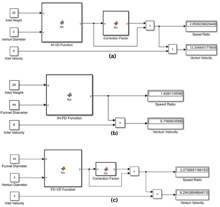
Figure 9. MATLAB/Simulink models that include the obtained primary surrogate equations and CF functions for: (a) IH–VD configuration, (b) IH–FD configuration, and (c) FD–VD configuration
After deriving the main surrogate equations and the CF functions, MATLAB/Simulink models were developed for each dataset as an individual subsystem within MATLAB Simulink. The individual models corresponding to the IH–VD, IH–FD, and FD–VD configurations are illustrated in Figure 9, respectively. The final corrected SR is obtained as
Final $\mathrm{SR}=S R$ in MATLAB $\times C F-$ function (11)
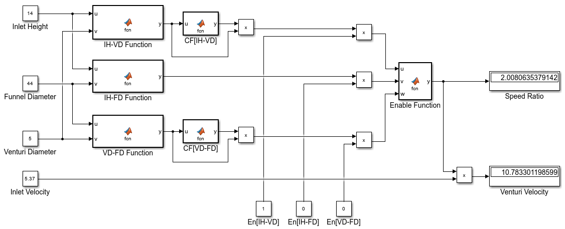
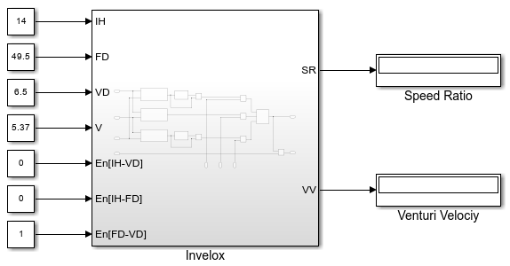
After applying the CFs, the final model's prediction accuracy improved significantly. When compared with the CFD results, the IH–VD model accuracy improved to 98.84%, and the FD–VD model achieved an accuracy of 99.12%. Now the developed three models required the user to operate them separately, and allowed tuning of only two geometric parameters at a time. To improve usability, a combined Simulink framework was developed, where, within a single interface, the IH, VD, FD, and inlet velocity can be adjusted simultaneously. In this combined system, each surrogate model is implemented as an individual subsystem block. To activate the desired model, three dedicated enable switches are used, which allow users to select and analyze a specific geometric configuration effortlessly. Figure 10 illustrates the complete combined Simulink model, and Figure 11 shows the block diagram of the final integrated model framework. The combined Simulink model illustrated in Figure 10 incorporates three parallel subsystem blocks that implement the IH–VD, IH–FD, and FD–VD surrogate equations along with their respective CFs. Three enable switches permit activation of only the desired configuration. The four input ports namely, IH, FD, VD, and inlet velocity are directly adjustable by the user. The model outputs the corrected SR. This structure offers a unified and accessible interface for efficient parametric studies.
Figure 10. Combined MATLAB/Simulink framework integrating the three surrogate model subsystems into a unified interface, featuring dedicated enable switches and multi-parameter tuning for IH, VD, FD, and inlet velocity
Figure 11. Block diagram of the combined MATLAB/Simulink framework integrating the three surrogate model subsystems into a unified interface, featuring dedicated enable switches and multi-parameter tuning for IH, VD, FD, and inlet velocity
3.3 Comparison with previous studies
The earlier single-parameter MATLAB model [32] considers only the IH as a variable while maintaining the remaining geometric parameters at fixed reference values. Consequently, its applicability to location-specific geometric optimisation is limited. In comparison to earlier models, the current framework enables simultaneous variation of two geometric parameters and integrates CFs based on a substantially larger CFD dataset comprising 250 cases. Compared to pure CFD analysis, the surrogate model is able to reduce computation time while maintaining an average predictive accuracy exceeding 98%. Therefore, rather than replacing CFD analysis, these features render the model highly suitable for rapid preliminary design and sensitivity analyses.
The existing basic MATLAB model of INVELOX allows the user to vary only the IH to examine the system performance. An improved CFD-informed MATLAB/Simulink surrogate model was developed and validated for the INVELOX system to address the flaws in the basic model and enable rapid, higher-accuracy prediction of the SR. In this article, surrogate mathematical models were made based on CFD simulations generated data for three parameter pairs: IH–VD, IH–FD, and FD–VD. The prediction capability of those mathematical models was quite similar to the CFD results, with accuracies of 98.02%, 98.64%, and 97.88% for the IH–VD, IH–FD, and FD–VD models, respectively. Incorporation of developed CF functions improves accuracy to 98.84% and 99.12% for the IH–VD and FD–VD models, but does not enhance the IH–FD model accuracy. Those mathematical models with respective CF functions were used to develop this proposed MATLAB/Simulink model of the INVELOX system. This model provides a faster and easier way to assess preliminary designs and improve performance compared to traditional CFD analysis.
Finally, the developed MATLAB/Simulink surrogate model provides a computationally efficient tool for rapid preliminary evaluation of the INVELOX SR under simultaneous variation of the three key geometric parameters. The present validation is purely numerical and limited to low-to-moderate wind speeds. Experimental validation and multi-speed extension remain necessary before the model can be applied with full confidence in practical engineering design. Nevertheless, the developed framework offers a useful complementary approach to conventional CFD for early-stage design exploration of INVELOX wind systems in low-to-moderate wind regimes. Future work will add power output predictions and experimental validation to make the model even more practical.
|
CF |
Correction factor(dimensionless) |
|
FD |
Funnel diameter (ft) |
|
IH |
Inlet height (ft) |
|
VD |
Venturi diameter (ft) |
|
SR |
Speed ratio (dimensionless) |
|
Greek symbols |
|
|
a |
coefficient of series function |
|
b |
coefficient of series function |
|
ε |
Turbulent dissipation rate |
|
θ |
Frequency parameter in the Fourier series |
[1] Stern, N. (2009). The Global Deal: Climate Change and the Creation of a New Era of Progress and Prosperity. PublicAffairs. https://www.amazon.com/Global-Deal-Creation-Progress-Prosperity/dp/1586486691.
[2] UNFCCC. (2016). The Paris Agreement. United Nations Framework Convention on Climate Change. https://unfccc.int/process-and-meetings/the-paris-agreement/the-paris-agreement, accessed on 26 Apr. 2023.
[3] Sadorsky, P. (2021). Wind energy for sustainable development: Driving factors and future outlook. Journal of Cleaner Production, 289: 125779. https://doi.org/10.1016/j.jclepro.2020.125779
[4] Goal 7: Affordable and Clean Energy, Sustainable Development Goals, United Nations Department of Economic and Social Affairs. https://sdgs.un.org/goals/goal7.
[5] Sørensen, J.N. (2011). Aerodynamic aspects of wind energy conversion. Annual Review of Fluid Mechanics, 43: 427-448. https://doi.org/10.1146/annurev-fluid-122109-160801
[6] Kumar, A., Khan, M.Z.U., Pandey, B. (2018). Wind energy: A review paper. Gyancity Journal of Engineering and Technology, 4(2): 29-37. https://doi.org/10.21058/gjet.2018.42004
[7] Energy institute, statistical review of world energy. (2026). In 75th ed., London, U.K. https://www.energyinst.org/statistical-review.
[8] IRENA. (2025). Renewable capacity statistics 2025. https://www.irena.org/Publications/2025/Mar/Renewable-capacity-statistics-2025.
[9] IEA. (2022). World energy outlook 2022. https://iea.blob.core.windows.net/assets/830fe099-5530-48f2-a7c1-11f35d510983/WorldEnergyOutlook2022.pdf, accessed on Apr. 27, 2023.
[10] Azevêdo, R.O., Rotela Junior, P., Chicco, G., Aquila, G., Rocha, L.C.S., Peruchi, R.S. (2020). Identification and analysis of impact factors on the economic feasibility of wind energy investments. International Journal of Energy Research, 45(3): 3671-3697. https://doi.org/10.1002/er.6109
[11] McKenna, R., Pfenninger, S., Heinrichs, H., et al. (2022). High-resolution large-scale onshore wind energy assessments: A review of potential definitions, methodologies and future research needs. Renewable Energy, 182: 659-684. https://doi.org/10.1016/j.renene.2021.10.027
[12] Chitura, A.G., Mukumba, P., Shambira, N. (2025). Increased velocity (INVELOX) wind delivery system: A review of performance enhancement advances. Wind, 5(3): 19. https://doi.org/10.3390/wind5030019
[13] Allaei, D., Andreopoulos, Y. (2014). INVELOX: Description of a new concept in wind power and its performance evaluation. Energy, 69: 336-344. https://doi.org/10.1016/j.energy.2014.03.021
[14] Hosseini, S.R., Ganji, D.D. (2020). A novel design of nozzle-diffuser to enhance performance of INVELOX wind turbine. Energy, 198: 117082. https://doi.org/10.1016/j.energy.2020.117082
[15] Suthagar, S., Kumaran, T., Gowtham, G., Maridurai, T., Sathish, T., Deivanayagi, S. (2021). Computational analysis of INVELOX wind turbine to analyze the venturi velocity by change the parameter of diffuser. Materials Today: Proceedings, 46: 4245-4249. https://doi.org/10.1016/j.matpr.2021.03.049
[16] Sotoudeh, F., Kamali, R., Mousavi, S.M. (2019). Field tests and numerical modeling of INVELOX wind turbine application in low wind speed region. Energy, 181: 745-759. https://doi.org/10.1016/j.energy.2019.05.186
[17] Farokhzade, A., Maghrebi, M.J. (2021). Inlet parameters effects of Invelox on the aerodynamic performance using numerical simulation. Journal of Applied Fluid Mechanics, 14(5): 1511-1520. https://doi.org/10.47176/jafm.14.05.32554
[18] Gohar, G.A., Manzoor, T., Ahmad, A., et al. (2019). Design and comparative analysis of an INVELOX wind power generation system for multiple wind turbines through computational fluid dynamics. Advances in Mechanical Engineering, 11(4): 168781401983147. https://doi.org/10.1177/1687814019831475
[19] Anbarsooz, M., Hesam, M.S., Moetakef-Imani, B. (2017). Numerical study on the geometrical parameters affecting the aerodynamic performance of Invelox. IET Renewable Power Generation, 11(6): 791-798. https://doi.org/10.1049/iet-rpg.2016.0668
[20] Ayaz, A., Israr, A., Khan, M.Z. (2023). Numerical and experimental investigation of geometric parameters influence on power generation of INVELOX wind turbine. Energy for Sustainable Development, 77: 101329. https://doi.org/10.1016/j.esd.2023.101329
[21] Gordievsky, E., Miroshnichenko, A., Solomin, E. (2020). Wind turbine MATLAB simulation model. In 2020 International Conference on Industrial Engineering, Applications and Manufacturing (ICIEAM), Sochi, Russia, pp. 1-5. https://doi.org/10.1109/icieam48468.2020.9112076
[22] Ghorani, M.M., Karimi, B., Mirghavamia, S.M., Saboohi, Z. (2023). A numerical study on the feasibility of electricity production using an optimized wind delivery system (Invelox) integrated with a horizontal axis wind turbine (HAWT). Energy, 268: 126643. https://doi.org/10.1016/j.energy.2023.126643
[23] Chen, X., Wang, P., Zhang, D.Y. (2017). Surrogate-based multidisciplinary design optimization of an autonomous underwater vehicle hull. In 2017 16th International Symposium on Distributed Computing and Applications to Business, Engineering and Science (DCABES), Anyang, China, pp. 191-194. https://doi.org/10.1109/DCABES.2017.48
[24] Parsa, S.M. (2025). Physics-informed machine learning meets renewable energy systems: A review of advances, challenges, guidelines, and future outlooks. Applied Energy, 402: 126925. https://doi.org/10.1016/j.apenergy.2025.126925
[25] Giacomini, M., Díez, P. (2026). Surrogates for physics-based and data-driven modelling of parametric systems: Review and new perspectives. Archives of Computational Methods in Engineering. https://doi.org/10.1007/s11831-026-10552-4
[26] Chen, Y., Zhang, D., Li, X., et al. (2023). Surrogate models for twin-VAWT performance based on Kriging and artificial neural networks. Ocean Engineering, 273: 113947. https://doi.org/10.1016/j.oceaneng.2023.113947
[27] Pettas, V., Cheng, P.W. (2024). Surrogate modeling and aeroelastic analysis of a wind turbine with down-regulation, power boosting, and IBC capabilities. Energies, 17(6): 1284. https://doi.org/10.3390/en17061284
[28] Witter, S., Roth, J., Schelenz, R., Jacobs, G. (2025). Creating a real-time capable surrogate model of a wind turbine using machine learning. Wind Energy, 28(11): e70070. https://doi.org/10.1002/we.70070
[29] Baisthakur, S., Fitzgerald, B. (2024). Physics-informed neural network surrogate model for bypassing blade element momentum theory in wind turbine aerodynamic load estimation. Renewable Energy, 224: 120122. https://doi.org/10.1016/j.renene.2024.120122
[30] Chen, R., Qin, D., Liu, C. (2023). Dynamic modelling and dynamic characteristics of wind turbine transmission gearbox-generator system electromechanical-rigid-flexible coupling. Alexandria Engineering Journal, 65: 307-325. https://doi.org/10.1016/j.aej.2022.10.036
[31] Martin, G.E., Verbrugge, B., Hasan, M.M., El Baghdadi, M., Romano, C., Hegazy, O. (2025). Artificial intelligence-driven thermal management in electric vehicle traction inverters: Cooling system optimization and real-time temperature prediction. IEEE Access, 13: 167632-167648. https://doi.org/10.1109/ACCESS.2025.3612315
[32] Billah, S.M.B., Qasim, S. (2019). Development of MATLAB Simulink model of Invelox to analyze the impact of inlet height on speed ratio. In 2019 International Conference on Energy and Power Engineering (ICEPE), Dhaka, Bangladesh, pp. 1-5. https://doi.org/10.1109/CEPE.2019.8726795
[33] What is meshing? https://simutechgroup.com/why-is-meshing-important-for-fea-fluid-simulations/.
[34] Zhang, C.F., An, S., Wang, W., Lin, D.H. (2021). A novel meshing method based on adaptive size function and moving mesh for electromagnetic finite element analysis. Symmetry, 13(2): 254. https://doi.org/10.3390/sym13020254
[35] Gorman, J., Bhattacharyya, S., Cheng, L.J., Abraham, J.P. (2021). Turbulence models commonly used in CFD. In Applications of Computational Fluid Dynamics Simulation and Modeling. IntechOpen. https://doi.org/10.5772/intechopen.99784
[36] Bangladesh Meteorological Department (BMD), “Normal Wind Speed (m/s),” 2016. https://www.bmd.gov.bd/file/2016/08/17/pdf/6206.pdf.