
Kukuh Yudhistiro* | Ruri S. Basuki | Nova Rijati
© 2026 The authors. This article is published by IIETA and is licensed under the CC BY 4.0 license (http://creativecommons.org/licenses/by/4.0/).
OPEN ACCESS
The Gabor Wavelet provides multi-orientation filtering for edge-based boundary detection, but its kernel parameters are normally fixed across an entire image. This paper presents the Adaptive Imaginary Gabor Wavelet (A-GWi), a handcrafted method that sets the centre frequency and scale of an imaginary-only Gabor kernel at every pixel from a closed-form mapping of a local gradient activity estimate, without training and without a graphics processing unit (GPU). Evaluation follows the Berkeley protocol on the Berkeley Segmentation Dataset 500 (BSDS500) and the Unified Dataset for Edge Detection (UDED). A-GWi reaches an optimal dataset scale (ODS) F-measure of 0.534 on BSDS500 and 0.668 on UDED, against 0.417 and 0.580 for the static imaginary Gabor Wavelet and 0.397 and 0.507 for the Gabor Wavelet Complex (GWC). The margin over both static baselines is significant on both datasets, while the difference against a gradient-magnitude Canny baseline is not. An ablation shows that a static kernel at the lower frequency bound reaches the same accuracy, so the per-pixel mechanism selects an effective operating point without manual tuning rather than improving on the best static configuration. The method runs on a single processor thread at 604 ms per image.
adaptive edge detection, Gabor Wavelet, imaginary-only filtering, spatially varying convolution, local density modulation
Edge-based boundary detection, which is frequently enhanced by recent methods like adaptive thresholding [1] and multi-scale selection [2], locates pixels where image intensity changes abruptly. This fundamental process supports medical image inspection, industrial material classification, and agricultural image analysis in which objects appear at varying local densities [3]. Classical detectors such as Canny [4], Sobel and Feldman [5], and the Laplacian of Gaussian [6], together with standard Gabor Wavelets [7, 8], apply fixed-parameter filters uniformly across an image. Even when recent works extend these detectors with the aforementioned adaptive thresholding [1, 9] or multi-scale selection [2, 10], the underlying convolution kernel remains spatially invariant. A single kernel cannot resolve fine boundaries in cluttered regions and capture broad contours in homogeneous regions at the same time, which produces spatially non-uniform responses that lower precision, recall, and the F-measure.
Adaptive approaches act on the threshold [1, 9, 11], on the choice of filter scale at the block level [2, 10], or on Gabor parameters learned inside a convolutional network [12-16]. A related line embeds Gabor filters in deep networks as learnable or fixed front ends [17-21]. None of these sets the kernel parameters of a handcrafted detector at each pixel from a local estimate of image content, and the learned variants require labelled data and a graphics processing unit (GPU). Section 2 reviews these strategies, and Table 1 positions the present formulation against them.
The imaginary-only Gabor Wavelet (GWi) halves the convolution count of the complex Gabor Wavelet (GWC) while preserving the edge-sensitive antisymmetric response, and it inherits the same spatial-invariance limitation. This paper asks whether the kernel parameters of that formulation can be set per pixel in closed form, and what such a mechanism contributes once its effect is separated from the effect of the operating point it selects. The proposed method, the Adaptive Imaginary Gabor Wavelet (A-GWi), modulates the centre frequency and the Gaussian scale at each pixel through a sigmoid mapping of a Sobel-derived local gradient activity estimate. Table 1 places the mechanism against prior adaptation strategies along four dimensions.
This work makes three contributions. First, it proposes a handcrafted spatially varying Gabor formulation in which the kernel frequency and scale are computed at each pixel in closed form, without training. Second, it reports an ablation that separates the contribution of the per-pixel mechanism from the contribution of the operating point, together with two negative controls on the driving signal. Third, it reports an evaluation under the Berkeley protocol on two datasets against five handcrafted baselines, with bootstrap confidence intervals and paired significance tests for every comparison.
Table 1. Adaptation strategies in prior edge detectors and in the proposed method, positioned along four dimensions
|
Method Family |
What is Adapted |
Granularity |
Training Required |
Closed Form |
|
Threshold-based [1, 9, 11] |
Binarization threshold |
Image or block |
No |
Yes |
|
Multi-scale selection [2, 10] |
Filter bank selection |
Image or block |
No |
Yes |
|
Fingerprint enhancement [22] |
Gabor frequency and orientation |
Block |
No |
Yes |
|
Gabor convolutional network [15, 16] |
Gabor parameters |
Layer |
Yes |
No |
|
Adaptive Gabor network [14] |
Gabor parameters |
Channel |
Yes |
No |
|
Learnable Gabor edge layer [12] |
Gabor parameters |
Layer |
Yes |
No |
|
Deformable Gabor network [13] |
Sampling locations |
Pixel |
Yes |
No |
|
Dynamic filter network [23] |
Whole kernel |
Pixel |
Yes |
No |
|
Pixel-adaptive convolution [24] |
Kernel modulation |
Pixel |
Yes |
No |
|
This work |
Gabor frequency and scale |
Pixel |
No |
Yes |
2.1 Imaginary-only Gabor filtering
The complex two-dimensional Gabor Wavelet [8, 25] is a sinusoid modulated by a Gaussian envelope, following the receptive-field model of Daugman [7]. Under a rotation of the axes, it separates into a symmetric cosine part and an antisymmetric sine part, and the antisymmetric part responds maximally to step edges. The GWi retains only that component and takes the maximum absolute response over N orientations, which halves the convolution count of the GWC. Jiang et al. [26] reduced cost instead by simplifying the kernel coefficients, and Lee et al. [27] analyse the cost of dense multi-orientation banks directly. GWi uses a single global parameter set, which motivates the per-pixel formulation introduced here.
2.2 Adaptation in handcrafted detectors
Li and Xu [1], Kamanga [9], and Bradley and Roth [11] adapted the binarization threshold while the filter remains fixed. Li et al. [2] selected among preset Gabor scales, and Sun and Sun [10] adapt directional weighting. In each case, the adaptation acts on the threshold, the filter bank, or the weighting, and not on the kernel at each pixel. The closest handcrafted precedent is fingerprint enhancement [22], where Gabor frequency and orientation follow a local ridge-frequency estimate, although the adaptation is computed per block and the task differs. Deep detectors reach higher accuracy on natural-scene benchmarks [28-30], and Gabor structure appears inside task-specific networks for medical segmentation [31] and small-sample object detection [32], but all of these require training data and a GPU, so they occupy a different regime from the training-free setting studied here.
2.3 Spatially varying filtering
Spatially varying convolution applies a different kernel at each location. Dynamic filter networks [23], pixel-adaptive convolution [24], and deformable convolution [33] realise this inside learned networks. In crowd counting, density maps act as spatial priors for adaptive feature extraction [34-36], and the geometry-adaptive kernels of Zhang et al. [22] showed that filter parameters can be conditioned on a local statistic. That principle has not been applied to handcrafted Gabor edge detectors, which is what the present work does with a closed-form kernel driven by a local gradient activity estimate.
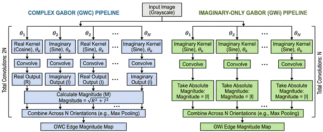
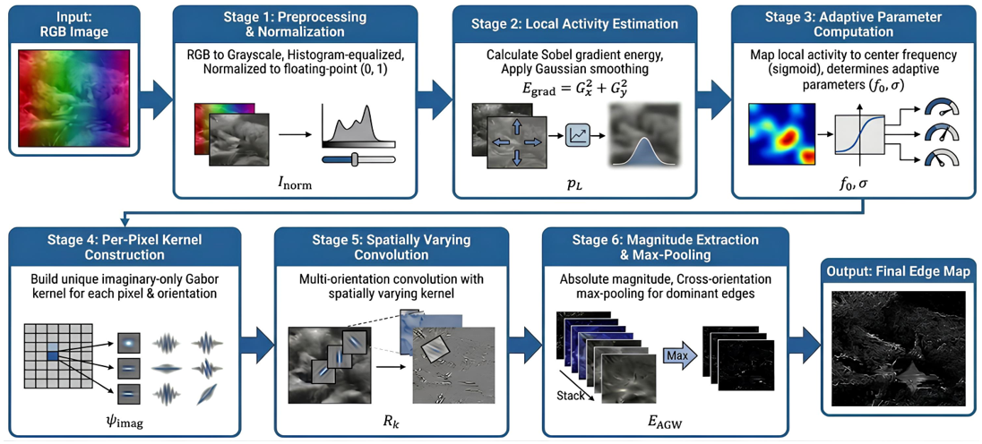
Figure 1 first compares the static GWC and GWi pipelines that motivate the imaginary-only design. Specifically, GWC convolves each orientation with both the real cosine kernel and the imaginary sine kernel and combines them by energy, which requires 2N convolutions for N orientations. In contrast, GWi convolves each orientation with the imaginary kernel only and takes the absolute magnitude, which requires N convolutions. By discarding the symmetric response, which mainly captures ridge-like features, GWi retains the antisymmetric response aligned with step edges at half the filtering cost [26]. The final cross-orientation maximum is identical in both pipelines, so the reduction is concentrated entirely in the per-orientation filtering stage. Based on this foundation, the proposed A-GWi method consists of six stages, as shown in Figure 2.
Figure 2 shows the six processing stages: preprocessing; local gradient activity estimation; adaptive parameter computation; per-pixel imaginary kernel construction; spatially varying multi-orientation convolution; and magnitude extraction with cross-orientation maximum pooling. The adaptive parameters are computed before convolution and vary per pixel, which is the mechanism that turns a static filter bank into a spatially varying convolution. The stages are described next with their governing equations.
3.1 Stage 1: Preprocessing
The colour input is converted to grayscale with ITU-R BT.601 coefficients, as given in Eq. (1), where R, G, and B denote the red, green, and blue channels.
$I_{\text {gray }}(u, v)=0.299 R+0.587 G+0.114 B$ (1)
The grayscale image is then contrast-enhanced by histogram equalization and divided by 255, as in Eq. (2), which places the intensity values in the floating-point range from 0 to 1 and simplifies the subsequent computation.
$I_{\text {norm }}(u, v)=$ HistEq $\left(I_{\text {gray }}\right) / 255$ (2)
The same preprocessed image is supplied to every method compared in Section 5, so that the filtering stage is the only difference between conditions.
3.2 Stage 2: Local gradient activity estimation
The local gradient activity is estimated from Sobel gradient energy and then smoothed. Eq. (3) computes the spatial derivative along the horizontal axis with a 5 × 5 Sobel aperture, and Eq. (4) computes the derivative along the vertical axis with the same aperture.
$G_x=\operatorname{Sobel}\left(I_{\text {norm }}, d x=1\right.$, ksize $\left.=5\right)$ (3)
$G_y=\operatorname{Sobel}\left(I_{\text {norm }}, d y=1\right.$, ksize $\left.=5\right)$ (4)
Eq. (5) gives the gradient energy at each pixel as the Euclidean norm of the two components, that is, the square root of the sum of their squares. Regions containing many objects or dense texture produce high energy values.
$E_{\text {grad }}(u, v)=\sqrt{ }\left(G x^2+G y^2\right)$ (5)
Eq. (6) gives the final estimate. The energy map is normalised by a minimum-maximum rescaling and then smoothed by a 5 × 5 Gaussian filter, so that the estimate is smooth and free of isolated gradient spikes.
$\rho L(u, v)=$ $GaussianBlur$$\left({minmax}\left(E_{\text {grad}}\right), 5 \times 5\right.$ (6)
High-activity regions map to a high value and homogeneous regions to a low value. Section 5.2 reports how closely the estimate tracks the ground-truth boundary density, and how closely it tracks local intensity contrast.
3.3 Stage 3: Adaptive kernel parameter computation
3.3.1 Adaptive frequency
Eq. (7) maps the activity estimate to a centre frequency through a sigmoid, which gives a bounded transition between the two frequency limits.
$\begin{gathered}f_{0, {adapt}}(u, v)= f_{\min }+\left(f_{\max }-f_{\min }\right) S\left(k_s\left(\rho L(u, v)-\rho_c\right)\right)\end{gathered}$ (7)
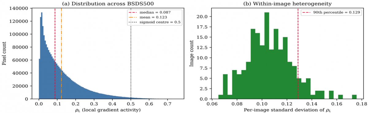
Here S(z) = 1 / (1 + exp(−z)), with steepness ks = 25, centre ρc = 0.5, and bounds fmin = 0.05 and fmax = 0.45 cycles per pixel. High-activity regions are intended to receive high frequencies and low-activity regions low frequencies. Because the median activity on the Berkeley Segmentation Dataset 500 (BSDS500) is 0.091, the sigmoid argument at the median is −10.2, so in practice most pixels receive a frequency close to fmin; Section 5.3 quantifies this.
3.3.2 Adaptive scale
Eq. (8) couples the Gaussian scale to the frequency through an inverse relation, so that a high frequency gives a narrow envelope and a low frequency a wide one.
$\sigma_{\text {adapt }}(u, v)=c / f_{0, \text { adapt }}(u, v), c=\sqrt{ }(\ln 2 / 2) / \pi$ (8)
The constant is c = 0.1874. This is proportional to the standard Gabor bandwidth relation but omits its factor of 3 at one octave, and the fixed 7 × 7 window truncates the envelope, retaining 88% of its mass at fmax and 11% at fmin. The coupling is therefore a scale-frequency relation rather than a constant-bandwidth constraint. Eq. (9) sets the two envelope widths, with the second axis scaled by the aspect ratio γ = 0.5 to sharpen orientation selectivity. Eq. (9) sets the two envelope widths. The width along the second axis is scaled by the aspect ratio γ = 0.5, which elongates the envelope and sharpens orientation selectivity.
$\sigma_x=\sigma_{ {adapt }}, \quad \sigma_y=\sigma_{ {adapt }} / \gamma$ (9)
3.4 Stage 4: Imaginary-only kernel construction
Eq. (10) constructs the imaginary-only Gabor kernel at each pixel for each orientation. The kernel is a Gaussian envelope multiplied by a sine carrier, which is the imaginary part of the complex Gabor kernel. The indices m and n run from −3 to 3 over the fixed 7 × 7 window, and the rotated indices are $m^{\prime}=m \cos \theta^{\circ}+n \sin \theta^{\circ}$ and $n^{\prime}=-m \sin \theta^o+n \cos \theta^o$. Removing the cosine component halves the number of convolutions without discarding edge information. The parameters are those computed in Stage 3, which makes the kernel unique at every location.
$\begin{gathered}\psi_{ {imag }}(m, n)= \exp \left[-0.5\left(\frac{m^{\prime 2}}{\sigma_x^2}+\frac{n^{\prime 2}}{\sigma_y^2}\right)\right] \sin \left(2 \pi f_{0, {adapt}} m^{\prime}\right)\end{gathered}$ (10)
3.5 Stage 5: Spatially varying multi-orientation convolution
Eq. (11) computes the response at orientation θo. Because the kernel parameters vary with position, the operation is a spatially varying convolution. The expression is written as a correlation; for the antisymmetric kernel used here, the convolution differs only in sign, so the two are equivalent after the absolute value is taken in Eq. (12). Pixels outside the image are supplied by reflection padding, which is applied identically to every method compared in Section 5.
$\begin{gathered}R_o(u, v)= \sum_m \sum_n I_{ {norm}}(u+m, v+n) \psi_{ {imag }}(m, n)\end{gathered}$ (11)
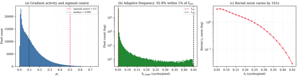
The kernel is not normalised, so its L2 norm varies with the centre frequency across the adaptive range, from 3.010 at fmin to 0.030 at fmax. This is reported here because it means that the response magnitude carries an amplitude scaling that is correlated with the activity estimate.
3.6 Stage 6: Magnitude extraction and maximum pooling
Eq. (12) takes the absolute value of each orientation response, and Eq. (13) selects the dominant orientation at each pixel.
$M_o(u, v)=\left|R_o(u, v)\right|$ (12)
$E_{A G W i}(u, v)=\max _o M_o(u, v)$ (13)
Eq. (14) rescales the output to the range from 0 to 1 by a minimum-maximum mapping computed per image. This step is stated explicitly because it determines what a single dataset-wide threshold means in the evaluation protocol of Section 4.2.
$\begin{gathered}E_{ {norm }}= \left(E_{ {AGWi }}-\min E_{{AGWi}}\right) /\left(\max E_{{AGWi }}-\min E_{ {AGWi}}\right)\end{gathered}$ (14)
3.7 Implementation settings
Table 2 lists every parameter used to produce the results in Section 5. The values are those in the released implementation, and Section 4.4 reports how the three sigmoid parameters were verified.
Table 2. Implementation settings of the Adaptive Imaginary Gabor Wavelet (A-GWi)
|
Parameter |
Symbol |
Value |
Parameter |
Symbol |
Value |
|
Minimum centre frequency |
fmin |
0.05 cycles/pixel |
Scale coefficient |
c |
0.1874 |
|
Maximum centre frequency |
fmax |
0.45 cycles/pixel |
Sobel aperture for activity |
– |
5 × 5 |
|
Sigmoid steepness |
ks |
25.0 |
Gaussian smoothing for activity |
– |
5 × 5 |
|
Sigmoid centre |
ρc |
0.5 |
Border handling |
– |
Reflection padding |
|
Number of orientations |
N |
8, spaced 22.5° |
Kernel normalisation |
– |
None applied |
|
Kernel size |
K |
7 × 7, fixed |
Response normalisation |
– |
Per-image, to [0, 1] |
|
Aspect ratio |
Γ |
0.5 |
Arithmetic precision |
– |
Double |
|
Phase offset |
ψ |
0 |
|
|
|
3.8 Algorithm and complexity
Algorithm 1 states the procedure. The adaptive parameters on lines 4 to 6 are recomputed at every pixel before the orientation loop, which is the operational difference from a static Gabor bank. For an image of height H and width W with N orientations and a fixed k × k window, the cost is O(HWNk²) with k = 7. The inner loops are compiled to machine code with a just-in-time compiler, and all timing in Section 5.7 is single-threaded.
|
Algorithm 1. Edge-based boundary detection with the Adaptive Imaginary Gabor Wavelet (A-GWi) |
|
Input: image I; orientations N = 8; window size k = 7; bounds [fmin, fmax] = [0.05, 0.45]; steepness ks = 25; sigmoid centre ρc = 0.5; aspect ratio γ = 0.5; coefficient c = 0.1874 Output: normalised edge magnitude map Enorm 1: Inorm ← equalizeHist (grayscale(I)) / 255 2: ρL ← GaussianBlur (minmax (sqrt (Gx² + Gy²)), 5 × 5), Eqs. (1) and (2) 3: for each pixel (u, v) do, Eqs. (3)-(6) 4: f0 ← fmin + (fmax − fmin) / (1 + exp (−ks (ρL (u, v) − ρc))) 5: σx← c / f0, Eq. (7) 6: σy ← σx / γ, Eq. (8) 7: mag ← 0, Eq. (9) 8: for each orientation θo ∈ {0, π/N, ..., (N−1) π/N} do 9: build ψimag (m, n) for m, n ∈ [−3, 3] from f0, σx, σy 10: R ← ∑m ∑nInorm (u+m, v+n) ψimag (m, n), reflection padding at borders, Eq. (10) 11: mag ← max (mag, |R|), Eq. (11) 12: end for, Eqs. (12) and (13) 13: EAGWi (u, v) ← mag 14: end for 15: Enorm ← (EAGWi − min EAGWi) / (max EAGWi − min EAGWi), Eq. (14) 16: return Enorm |
4.1 Datasets
Two benchmarks are used. The BSDS500 provides 200 test images with boundary annotations from multiple annotators, together with 100 validation images that are used only for parameter verification. It is the standard reference for edge-based boundary detection because of its size, its multi-annotator ground truth, and its coverage of natural-scene categories. The Unified Dataset for Edge Detection (UDED) provides 30 images with single-annotator ground truth, assembled from several public sources and covering a different distribution of scene content and resolution [37]. All 30 images are used, since the dataset has no training and test partition and contains no further images, so no selection was made by the authors. Because the method has no trained parameters, the second dataset is not a test of generalization in the sense used for learned models; it is a second evaluation set with different image statistics.
4.2 Evaluation protocol
The Berkeley protocol [38] is used because it is the standard for boundary-detection benchmarking and accommodates continuous edge maps. Predictions are swept over 99 thresholds in [0.01, 0.99], each thresholded map is thinned, and predicted edges are matched to ground truth within 0.0075 times the image diagonal. Matching is performed against each annotator separately: a predicted pixel counts as correct if it matches at least one annotator, recall counts are summed across annotators, and assignment within each annotator is one-to-one by increasing distance. For each threshold t, four counts are accumulated across the test set: matched and total ground-truth pixels, cntR(t) and sumR(t), and matched and total predicted pixels, cntP(t) and sumP(t). Recall, precision, and the F-measure follow in Eqs. (15) to (17).
$R(t)=\operatorname{cnt} R(t) / \operatorname{sum} R(t)$ (15)
$P(t)=\operatorname{cnt}P(t) / \operatorname{sum} P(t)$ (16)
$F(t)=2 P(t) R(t) /[P(t)+R(t)]$ (17)
The ODS is the maximum of Eq. (17) over the threshold grid, Eq. (18). The optimal image scale (OIS) F-measure selects the best threshold per image from that image's counts, accumulates the counts at those thresholds across the test set, and evaluates Eqs. (15) to (17) once, Eq. (19).
$O D S=\max _t F(t)$ (18)
$OIS$ $=F$ evaluated at $t_i{ }^*=\operatorname{argmax}_t F_i(t)$ (19)
Both metrics use the same accumulation, so OIS is not lower than ODS. Average precision (AP) is the area under the dataset-level precision-recall curve with precision made monotone. The previously submitted version used different accumulation schemes for the two metrics, which produced an inconsistent ordering for one method. As a check on the implementation, Canny reaches ODS = 0.533 on BSDS500 under this protocol, within 0.001 of the value obtained for the same detector definition in our previous work.
4.3 Baselines
Five handcrafted baselines are compared. Canny [4] and Sobel [5] are gradient-based detectors and serve as low-cost reference points; their sensitivity to threshold selection is documented separately [39]. Phase Congruency [40] is a multi-scale detector that does not rely on a Gabor kernel. GWC [8] and GWi are the closest baselines because they share the Gabor structure with A-GWi but apply fixed parameters across the image, so the contrast against them isolates the effect of the per-pixel computation. Table 3 lists the configuration of each method. Canny is evaluated as the Gaussian-smoothed gradient magnitude before non-maximum suppression and hysteresis, so that all six methods produce continuous maps that the threshold sweep traverses identically. The value obtained is below the figure commonly cited for Canny on BSDS500 [40], which is obtained with non-maximum suppression applied internally and without histogram equalization.
Table 3. Baseline configurations
|
Method |
Filter Parameters |
Output |
|
Canny |
Gaussian σ = 1.4, Sobel aperture 3 |
Gradient magnitude, continuous |
|
Sobel |
Aperture 3 |
L2 gradient magnitude |
|
Phase Congruency |
4 scales, 6 orientations, minimum wavelength 3, multiplier 2.1, filter bandwidth 0.55, noise factor 2.0 |
Phase congruency map |
|
GWC |
k = 7, wavelength 4, σ = 0.56 × wavelength, γ = 0.5, N = 8 |
Energy of the real and imaginary pair, maximum over orientations |
|
GWi |
As GWC |
Absolute imaginary response, maximum over orientations |
|
A-GWi
|
See Table 2
|
Absolute imaginary response, maximum over orientations
|
All six methods receive identical input, grayscale conversion followed by histogram equalization and normalisation to [0, 1], and identical border handling, thinning, matching, and threshold sweep. The previously submitted version supplied Canny with the unequalized image and used zero padding for the two static Gabor baselines; both differences have been removed and all results recomputed.
4.4 Parameter verification
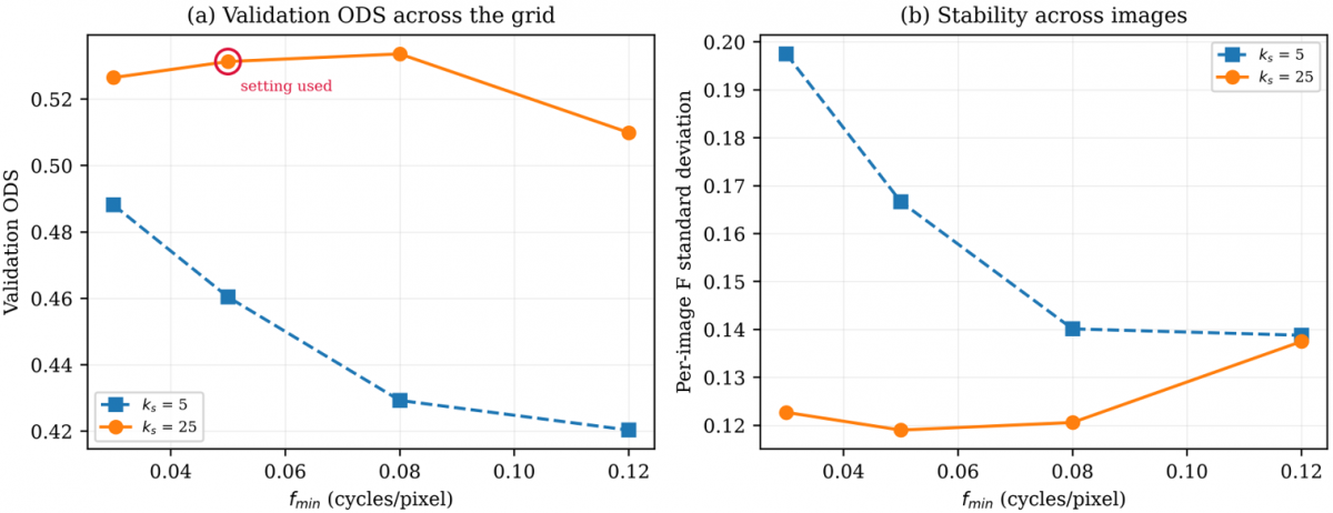
The sigmoid parameters were verified on the BSDS500 validation split of 100 images, which is separate from the test split used for all reported results. No test image was used at any stage of parameter selection. The search covered fmin in {0.03, 0.05, 0.08, 0.12} and ks in {5, 25}. The upper bound fmax was excluded because a separate sweep over {0.25, 0.35, 0.45, 0.55} changed ODS by 0.0009 in total, with no pairwise difference reaching significance. Table 4 reports the grid and Figure 3 plots it. The values used in this work, fmin = 0.05 and ks = 25, are supported by the grid. The steepness ks = 25 gives a higher validation ODS than ks = 5 at every fmin, by between 0.038 and 0.104. The lower bound fmin = 0.05 reaches a validation ODS of 0.531 against a best of 0.534 at fmin = 0.08, a difference of 0.002 against a standard error of approximately 0.012, so the two are not separable on this split and the original setting is retained.
Figure 3. Parameter verification on the BSD500 validation split. (a) Optimal dataset scale (ODS) F-measure across the search grid, with the setting used in this work circled (b) Standard deviation of the per-image F-measure
Table 4. Parameter verification on the BSD500 validation split of 100 images
|
fmin |
ks |
ODS |
OIS |
AP |
Per-Image F Standard Deviation |
|
0.03 |
5 |
0.488 |
0.545 |
0.410 |
0.197 |
|
0.03 |
25 |
0.526 |
0.558 |
0.489 |
0.123 |
|
0.05 |
5 |
0.460 |
0.518 |
0.364 |
0.167 |
|
0.05 |
25 |
0.531† |
0.565 |
0.492 |
0.119 |
|
0.08 |
5 |
0.429 |
0.488 |
0.333 |
0.140 |
|
0.08 |
25 |
0.534 |
0.567 |
0.484 |
0.121 |
|
0.12 |
5 |
0.420 |
0.480 |
0.321 |
0.139 |
|
0.12 |
25
|
0.510
|
0.551
|
0.429
|
0.137
|
One property of the grid is worth noting. At ks = 5 the sigmoid transition is wider, so the modulation is active at more pixels. The validation ODS is lower at every fmin, and the per-image standard deviation is higher, between 0.139 and 0.197 against 0.119 to 0.137 at ks = 25. This is consistent with the ablation in Section 5.3, where making the modulation fully active also lowers accuracy.
4.5 Hardware and software
All methods run on the same single-threaded configuration on an Intel Core i5-14400 with 16 GB of memory, with the thread counts of the linear algebra and image processing libraries forced to one, so that runtime reflects algorithmic cost per image and not the degree of parallelism available on the host. The software stack is Python 3.13 with OpenCV 4.13, NumPy, scikit-image, and Numba.
5.1 Quantitative results
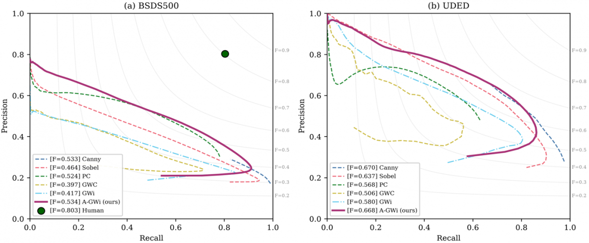
Table 5 reports the three metrics on the BSDS500 test set with 95% confidence intervals obtained by bootstrapping over images with 2,000 resamples. A-GWi attains the highest ODS at 0.534, above Canny at 0.533, Phase Congruency at 0.524, Sobel at 0.464, GWi at 0.417, and GWC at 0.397. The ordering is consistent with the design of the methods: the static Gabor banks sit below Sobel because their fixed kernel parameters do not match the per-pixel statistics of natural scenes, which produces over-detection in homogeneous regions and lowers precision. Table 6 reports the same metrics on UDED, where Canny attains the highest ODS at 0.670 and A-GWi follows at 0.668.
Table 5. Results on the BSD500 test set of 200 images, with 95% confidence intervals (CI) from 2,000 bootstrap resamples over images. Best value per column in bold
|
Method |
ODS |
95% CI |
OIS |
95% CI |
AP |
95% CI |
|
Canny |
0.533 |
[0.515, 0.552] |
0.562 |
[0.541, 0.582] |
0.493 |
[0.462, 0.523] |
|
Sobel |
0.464 |
[0.446, 0.483] |
0.503 |
[0.483, 0.524] |
0.406 |
[0.378, 0.436] |
|
Phase Congruency |
0.524 |
[0.508, 0.540] |
0.542 |
[0.526, 0.557] |
0.417 |
[0.397, 0.437] |
|
GWC |
0.397 |
[0.378, 0.417] |
0.465 |
[0.450, 0.481] |
0.277 |
[0.255, 0.302] |
|
GWi |
0.417 |
[0.399, 0.436] |
0.471 |
[0.455, 0.488] |
0.320 |
[0.297, 0.345] |
|
A-GWi |
0.534 |
[0.516, 0.553] |
0.566 |
[0.547, 0.584] |
0.485 |
[0.459, 0.512] |
Table 6. Results on the Unified Dataset for Edge Detection (UDED) of 30 images, with 95% confidence intervals from 2,000 bootstrap resamples over the images. Best value per column in bold
|
Method |
ODS |
95% CI |
OIS |
95% CI |
AP |
95% CI |
|
Canny |
0.670 |
[0.616, 0.720] |
0.729 |
[0.691, 0.758] |
0.680 |
[0.624, 0.732] |
|
Sobel |
0.637 |
[0.576, 0.696] |
0.713 |
[0.669, 0.747] |
0.647 |
[0.577, 0.712] |
|
Phase Congruency |
0.568 |
[0.532, 0.604] |
0.619 |
[0.589, 0.646] |
0.432 |
[0.391, 0.470] |
|
GWC |
0.507 |
[0.454, 0.575] |
0.586 |
[0.537, 0.633] |
0.366 |
[0.298, 0.455] |
|
GWi |
0.580 |
[0.524, 0.631] |
0.657 |
[0.617, 0.690] |
0.532 |
[0.472, 0.590] |
|
A-GWi |
0.668 |
[0.616, 0.714] |
0.724 |
[0.686, 0.753] |
0.653 |
[0.604, 0.698] |
Table 7 reports the paired comparisons. A-GWi exceeds both static Gabor baselines on both datasets with p below 10⁻⁷ and effect sizes between medium and large on the Cliff scale [41], where values below 0.147 are negligible, below 0.33 small, and below 0.474 medium. The difference against Canny is not significant on either dataset, at p = 0.82 on BSDS500 and p = 0.82 on UDED, so the two are not separable on this evidence. Against Phase Congruency the effect size differs between datasets, negligible on BSDS500 at 0.137 and medium on UDED at 0.442. The confidence intervals on UDED are wide because the dataset contains 30 images, and the interval for A-GWi overlaps those of Canny and Sobel. Figure 4 plots the precision-recall curves for both datasets.
Table 7. Paired comparison against the Adaptive Imaginary Gabor Wavelet (A-GWi) using the Wilcoxon signed-rank test [42] on per-image F-measures at the optimal dataset scale (ODS) threshold. The effect size is the Cliff delta [41]
|
Comparison |
Dataset |
Median Difference |
p |
Cliff delta |
Effect |
|
A-GWi vs GWC |
BSDS500 |
+0.123 |
3.6 × 10⁻³² |
+0.540 |
Large |
|
A-GWi vs GWi |
BSDS500 |
+0.106 |
8.7 × 10⁻³⁴ |
+0.474 |
Medium |
|
A-GWi vs Sobel |
BSDS500 |
+0.058 |
3.4 × 10⁻²⁸ |
+0.286 |
Small |
|
A-GWi vs Phase Congruency |
BSDS500 |
+0.021 |
1.8 × 10⁻⁸ |
+0.137 |
Negligible |
|
A-GWi vs Canny |
BSDS500 |
+0.002 |
0.82 |
+0.003 |
Not significant |
|
A-GWi vs GWC |
UDED |
+0.147 |
3.5 × 10⁻⁸ |
+0.578 |
Large |
|
A-GWi vs GWi |
UDED |
+0.094 |
1.9 × 10⁻⁹ |
+0.456 |
Medium |
|
A-GWi vs Phase Congruency |
UDED |
+0.103 |
1.9 × 10⁻⁴ |
+0.442 |
Medium |
|
A-GWi vs Sobel |
UDED |
+0.036 |
1.6 × 10⁻³ |
+0.116 |
Negligible |
|
A-GWi vs Canny |
UDED |
+0.000 |
0.82 |
−0.031 |
Not significant |
5.2 Validation of the activity estimate
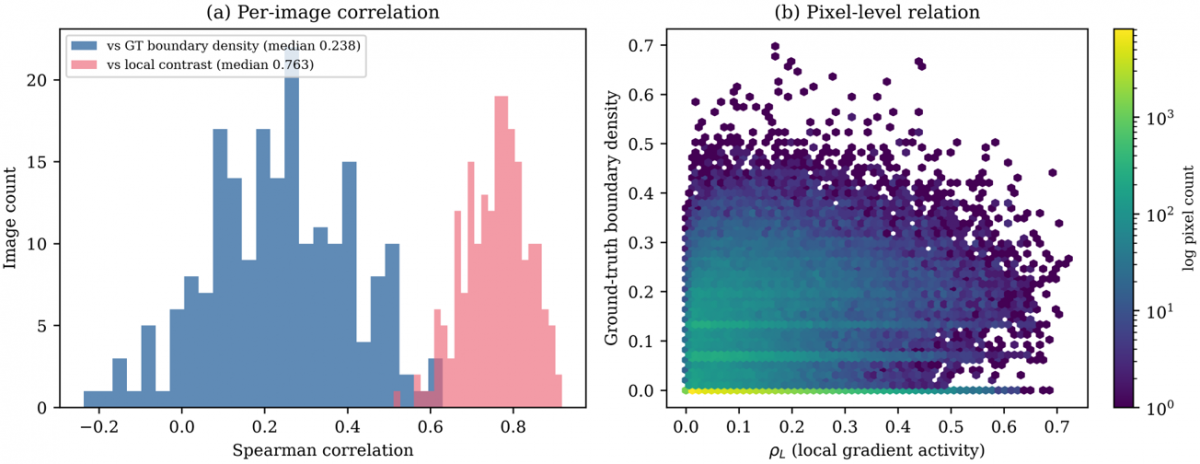
The quantity defined in Eqs. (3) to (6) is a smoothed gradient magnitude, so its relation to boundary density is not automatic and is verified here. Across the 200 BSDS500 test images, the Spearman correlation between the estimate and the local ground-truth boundary count in a 15 × 15 window has a median of 0.238, with an interquartile range from 0.111 to 0.361. The correlation with local intensity contrast in the same window has a median of 0.763, with an interquartile range from 0.705 to 0.811. The estimate therefore tracks local gradient activity rather than boundary density, and the term used throughout this paper reflects that.
Two consequences follow from the definition and are measured directly. In 2.76% of pixels, a high activity value coincides with a low boundary count, which occurs at isolated high-contrast edges. In 2.66% of pixels a high boundary count coincides with a low activity value, which occurs in dense low-contrast texture. Figure 5 shows the distribution of the estimate and Figure 6 shows the two correlations.
Figure 5. Local gradient activity on the BSD500, (a) distribution across the test set, with the median, the mean, and the sigmoid centre of Eq. (7) marked, (b) per-image standard deviation of the estimate, which shows that individual images contain both low-activity and high-activity regions
Figure 6. Validation of the local gradient activity estimate on the 200 test images of the BSD500, (a) per-image Spearman correlation of the estimate against the ground-truth boundary count in a 15 × 15 window and against local intensity contrast in the same window, (b) pixel-level relation between the estimate and the ground-truth boundary density
5.3 Ablation
Table 8 isolates the contribution of each element of the pipeline on the BSDS500 test set. Replacing the per-pixel computation with a static kernel at the lower frequency bound gives ODS = 0.535 against 0.534 for the full formulation, and the paired difference is not significant. Permuting the activity estimate spatially, which destroys its correspondence with image content while preserving its distribution, lowers ODS by only 0.004. Replacing the Sobel-based estimate with a local variance estimate raises ODS to 0.540. Evaluating the activity estimate directly as an edge map gives ODS = 0.508. Rank-normalising the estimate so that the sigmoid operates across its full range lowers ODS to 0.361.
Table 8. Ablation on the BSD500 test set. ODS denotes the optimal dataset scale F-measure (ODS)
|
Variant |
What is Changed |
ODS |
Difference |
p |
|
Static GWi, wavelength 4 |
No adaptation, high frequency |
0.417 |
−0.117 |
8.7 × 10⁻³⁴ |
|
Rank-normalised activity |
Modulation active across full range |
0.361 |
−0.173 |
2.1 × 10⁻³³ |
|
Activity as edge map |
Driving signal evaluated directly |
0.508 |
−0.026 |
4.1 × 10⁻¹⁵ |
|
Activity spatially permuted |
Negative control |
0.530 |
−0.004 |
4.8 × 10⁻² |
|
A-GWi, full |
Reference |
0.534 |
– |
– |
|
Static kernel at fmin |
No adaptation, low frequency |
0.535 |
+0.001 |
0.35 |
|
Activity from local variance |
Non-gradient estimator
|
0.540
|
+0.006
|
1.8 × 10⁻⁸
|
Two conclusions follow. First, the improvement over the static imaginary Gabor baseline at a wavelength of 4 pixels comes from the change in effective centre frequency rather than from per-pixel modulation. At the parameter setting used here, 92.8% of pixels receive a frequency within 1% of the lower bound, and the output correlates at 0.857 with a static bank at that frequency, as Figure 7 shows. Second, when the modulation is made active across the full range, accuracy falls, so the hypothesis that high-activity regions require high-frequency kernels is not supported on this benchmark. The per-pixel mechanism reaches the same operating point as the best static configuration without a manually selected centre frequency, rather than improving on it.
Figure 7. Behaviour of the adaptive mechanism at the setting reported in Table 2. (a) Distribution of the local gradient activity estimate against the sigmoid centre of Eq. (7). (b) Distribution of the resulting adaptive frequency on a logarithmic count axis; most pixels receive a frequency at the lower bound. (c) L2 norm of the imaginary Gabor kernel as a function of centre frequency inside the fixed 7 × 7 window
5.4 Activity-stratified analysis
The aggregate values in Tables 5 and 6 conflate performance across pixel contexts, so Tables 9 and 10 evaluate three activity strata separately. Stratum boundaries are the tertiles of the activity estimate on the BSDS500 training split, 0.053 and 0.146, applied as absolute thresholds to both evaluation sets so that no test statistic enters the analysis and the datasets remain comparable. Within each stratum, predicted and ground-truth pixels outside the mask are discarded before matching, so precision and recall are computed on the same population, Eq. (20). The per-stratum quantity Fs is not comparable with the aggregate value.
$F_s=\max _t F(t)$ restricted to $M_s$ (20)
Table 9. Activity-stratified F-measure on the BSD500
|
Method |
Low (7.1% of boundary pixels) |
Middle (25.1%) |
High (67.8%) |
|
Canny |
0.143 |
0.280 |
0.595 |
|
GWC |
0.116 |
0.236 |
0.479 |
|
GWi |
0.117 |
0.271 |
0.489 |
|
A-GWi
|
0.145
|
0.278
|
0.585
|
Table 10. Activity-stratified F-measure on the Unified Dataset for Edge Detection (UDED), using the same absolute stratum thresholds as Table 9. Abbreviations as in Table 9. Best value per stratum in bold
|
Method |
Low (9.0% of Boundary Pixels) |
Middle (28.4%) |
High (62.6%) |
|
Canny |
0.215 |
0.467 |
0.768 |
|
GWC |
0.149 |
0.368 |
0.650 |
|
GWi |
0.139 |
0.414 |
0.719 |
|
A-GWi |
0.218 |
0.462 |
0.743 |
Ground-truth boundary pixels are unevenly distributed across strata: on BSDS500, 7.1%, 25.1%, and 67.8% fall in the low, middle, and high strata, with a similar pattern on UDED, which is why the low-stratum values sit far below the aggregate. A-GWi exceeds both static Gabor baselines in every stratum on both datasets. The margin over GWi is +0.028, +0.007, and +0.096 on BSDS500 and +0.080, +0.049, and +0.024 on UDED, so the two datasets place the largest margin in different strata and the stratified view does not support a single account of where the difference arises. Canny is ahead in the middle and high strata on both datasets.
5.5 Error characterisation
Table 11 reports three quantities that address the behaviour of each detector more directly than the aggregate metrics. Precision at a fixed recall (PR) of 0.5 is defined in Eq. (21) and measures over-detection at a common operating point. The localisation error in Eq. (22) is the mean Euclidean distance between matched predicted pixels and their ground-truth counterparts at the ODS threshold. The edge width in Eq. (23) is the ratio of pixels above the threshold to pixels remaining after thinning, so a value near 1 means the response is already thin.
Table 11. Error characteristics on the BSD500
|
Method |
Precision at Recall 0.5 |
Localisation Error (pixels) |
Edge Width |
|
Canny |
0.589 (0.211) |
1.374 |
3.103 |
|
GWC |
0.329 (0.156) |
1.491 |
4.705 |
|
GWi |
0.405 (0.180) |
1.303 |
2.331 |
|
A-GWi
|
0.564 (0.190)
|
1.394
|
2.803
|
$P R=P\left(t^*\right), R\left(t^*\right)=0.5$ (21)
$L_{e r r}=(1 / \mid$ $Match$ $\mid) \sum\|p-g\|$ (22)
$W_{{edge }}=\left|\left\{(u, v): E_{ {norm}} \geq t_{ {ODS}}\right\}\right| /\left|P\left(t_{ {ODS}}\right)\right|$ (23)
Precision at fixed recall (PR) rises from 0.405 for GWi to 0.564 for A-GWi, which quantifies the reduction in spurious response that the qualitative comparison in Section 5.6 describes. The localisation error lies between 1.30 and 1.49 pixels for all four methods, well inside the matching tolerance of 4.3 pixels for a 481 × 321 image, so localisation accuracy is not a source of difference here. The edge width is 2.33 for GWi and 2.80 for A-GWi, which reflects the wider Gaussian envelope of the kernel that the mechanism selects at most pixels. The difference between the two methods therefore comes from response selectivity rather than from response width.
5.6 Qualitative comparison
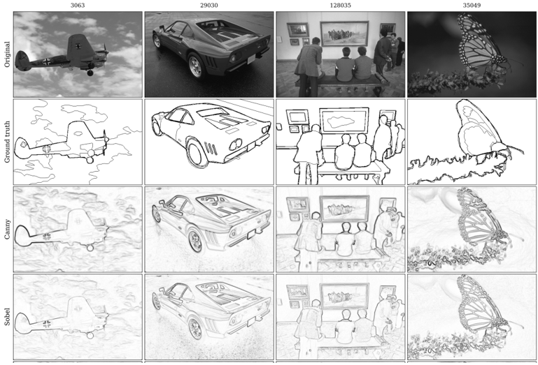
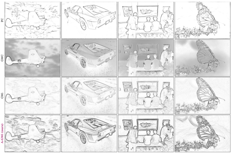
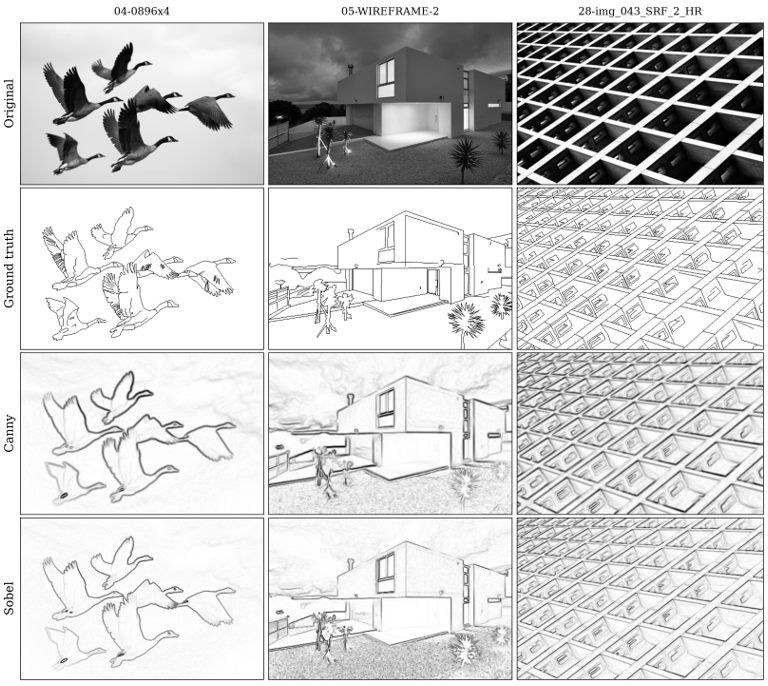
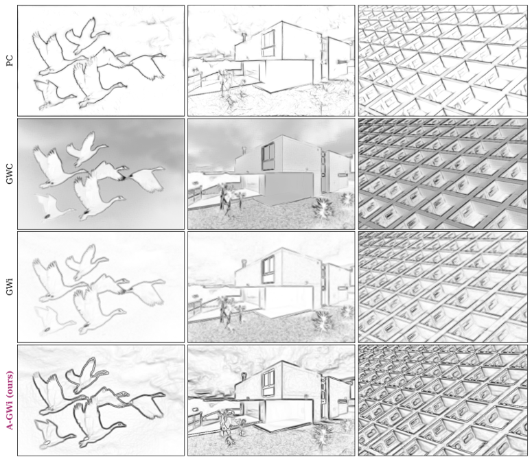
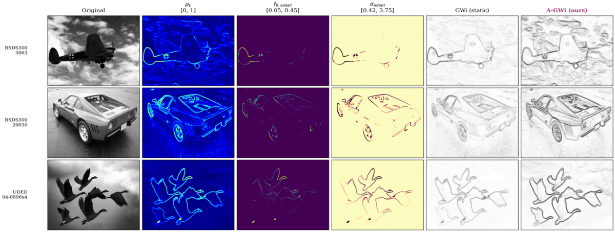
Figures 8 and 9 show the six detectors on representative images, and Figure 10 shows the per-pixel parameters with the resulting edge maps. A-GWi produces fewer spurious responses in homogeneous regions than either static Gabor baseline, which Table 11 quantifies as precision at fixed recall, but its response is not narrower than that of GWi, so the difference lies in selectivity rather than in the spatial extent of the response. The frequency map in Figure 10 is close to uniform at the lower bound over most of each image, which is the visual counterpart of the ablation in Table 8; the activity map itself concentrates along object boundaries, so the driving signal is informative even though the mapping in Eq. (7) compresses it to a narrow frequency range at this setting.
(a)
(b)
Figure 8. Qualitative comparison on the BSD500 for image identifiers 3063, 29030, 128035, and 35049 Edge maps are shown as dark edges on a light background, (a) Rows: original image, ground truth, Canny, Sobel (b) Phase Congruency, Gabor Wavelet Complex (GWC), imaginary-only Gabor Wavelet (GWi), and Adaptive Imaginary Gabor Wavelet (A-GWi)
(a)
(b)
5.7 Runtime
Table 12 reports the mean per-image runtime on the 200 BSDS500 test images, measured single-threaded with the just-in-time compiler warmed before timing. Each image is timed three times and the minimum is retained, which limits the influence of background system load; the standard deviation for A-GWi is 5.82 ms, under 1% of the mean. The gradient operators are fastest, at 1.66 ms for Sobel and 2.28 ms for Canny. The static Gabor banks are an order of magnitude slower because they filter eight orientations: GWi at 15.54 ms and GWC at 33.70 ms. The ratio of 2.17 between them matches the ratio of 2N to N convolutions and confirms that the imaginary-only formulation halves the filtering cost. Phase Congruency runs at 402.16 ms. A-GWi is the slowest at 604.41 ms, because it builds a kernel at every pixel rather than reusing a precomputed bank.
Table 12. Mean per-image runtime on the 200 test images of the BSD500, single-threaded on an Intel Core i5-14400
|
Method |
Mean (ms) |
Standard Deviation (ms) |
Minimum (ms) |
Maximum (ms) |
Speed Relative to A-GWi |
|
Sobel |
1.66 |
0.08 |
1.52 |
2.28 |
363 × faster |
|
Canny |
2.28 |
0.10 |
2.12 |
2.65 |
265 × faster |
|
GWi |
15.54 |
0.55 |
14.85 |
18.43 |
38.9 × faster |
|
GWC |
33.70 |
0.95 |
32.37 |
36.08 |
17.9 × faster |
|
Phase Congruency |
402.16 |
8.33 |
390.31 |
426.12 |
1.5 × faster |
|
A-GWi |
604.41
|
5.82
|
596.49
|
629.34
|
1.0 × (reference)
|
Within the multi-scale family, A-GWi is 1.5 times slower than Phase Congruency while reaching a higher ODS on BSDS500. Against Canny it is 265 times slower for an accuracy difference that is not significant on either dataset, so the gradient operator is the more efficient choice where a single edge magnitude map is the required output; the per-pixel formulation is of interest where the multi-orientation response is used downstream or where kernel parameters must be set without manual tuning.
5.8 Limitations
Three limitations follow from the results. The per-pixel construction prevents the separable optimisation available to static kernels, and at 604 ms per image it is 265 times slower than a gradient baseline of comparable accuracy. The mechanism does not improve accuracy over the best static configuration on these benchmarks, and making the modulation fully active lowers accuracy, so the hypothesis relating activity to frequency is not confirmed; the supported claim is that the mechanism reaches that configuration without manual tuning. The evaluation is limited to natural-scene benchmarks, and validation on dense agricultural grain imagery is left for future work.
This paper presented the A-GWi, a handcrafted formulation in which the centre frequency and scale of an imaginary-only Gabor kernel are set at every pixel in closed form from a local gradient activity estimate, without training and without a GPU. The method exceeds both static Gabor baselines on both datasets with medium to large effect sizes, in a comparison that is controlled in the sense that the three methods share the kernel structure, the orientation count, the window size, and the preprocessing. Against a gradient-magnitude Canny baseline the difference is not significant on either dataset.
The ablation qualifies what the mechanism contributes. A static kernel at the lower frequency bound reaches the same accuracy as the full formulation, so the improvement over the static baseline at a wavelength of 4 pixels comes from the change in effective centre frequency rather than from per-pixel modulation, and making the modulation active across the full range lowers accuracy. What the mechanism provides is an effective operating point without a manually selected centre frequency, which is a weaker but supported claim. The adaptation is deterministic and reproducible, with no random initialisation and no learned weights, and the pipeline runs on a single processor thread. It is not real time, and no embedded platform was tested.
Future work follows three directions. Kernel quantization with a discrete lookup table over activity levels can reduce the per-pixel cost towards real-time throughput. Recentring the sigmoid mapping on the empirical distribution of the activity estimate, and re-examining the direction of the frequency relation, may allow the mechanism to contribute beyond parameter selection. The extension to dense agricultural grain imagery is the motivating downstream application, where the method is intended to support kernel counting and aflatoxin screening in shelled corn. In earlier work on that application, aflatoxin fluorescence was detected under ultraviolet illumination with a simplified Gabor wavelet, where per-image counting accuracy ranged from 81% to 97% and the residual error came from the boundaries of overlapping kernels rather than from the fluorescence signal [43].
Conceptualization, K. Yudhistiro, R.S. Basuki, and N. Rijati; methodology and software, K. Yudhistiro; validation, all authors; formal analysis, data curation, and visualization, K. Yudhistiro; writing, original draft, K. Yudhistiro; writing, review and editing, R.S. Basuki and N. Rijati; supervision, R.S. Basuki and N. Rijati.
This work is supported by Universitas Dian Nuswantoro, Semarang, Indonesia, for research facilities and support.
All evaluation code, ablation scripts, runtime logs, and figure-generation scripts are released at https://github.com/kukuhyudhistiro/localgradientactivity- to enable reproduction.
|
c |
scale coefficient in the frequency-scale relation, dimensionless |
|
cntP |
number of matched predicted pixels, dimensionless |
|
cntR |
number of matched ground-truth pixels, dimensionless |
|
EAGWi |
edge magnitude map of the proposed method, dimensionless |
|
Egrad |
gradient energy magnitude, dimensionless |
|
Enorm |
normalised edge magnitude map, dimensionless |
|
F |
F-measure, dimensionless |
|
Fs |
stratum F-measure, dimensionless |
|
f0,adapt |
per-pixel adaptive centre frequency, cycles per pixel |
|
fmax |
upper bound of the adaptive frequency, cycles per pixel |
|
fmin |
lower bound of the adaptive frequency, cycles per pixel |
|
G |
green channel of a colour image, range 0 to 255 |
|
Gx, Gy |
Sobel gradient components, dimensionless |
|
H, W |
image height and width, pixels |
|
I |
input image |
|
Igray |
grayscale image, range 0 to 255 |
|
Inorm |
normalised grayscale image, range 0 to 1 |
|
k |
kernel size, pixels |
|
ks |
sigmoid steepness, dimensionless |
|
Lerr |
localisation error, pixels |
|
Mo |
absolute response at orientation o, dimensionless |
|
Ms |
binary mask of activity stratum s, dimensionless |
|
m, n |
kernel sample indices, pixels |
|
m′, n′ |
kernel indices rotated by the orientation angle, pixels |
|
N |
number of orientations, dimensionless |
|
ODS |
optimal dataset scale F-measure, dimensionless |
|
OIS |
optimal image scale F-measure, dimensionless |
|
o |
orientation index, dimensionless |
|
P |
precision, dimensionless |
|
R |
recall; also the red channel of a colour image, range 0 to 255 |
|
Ro |
convolution response at orientation o, dimensionless |
|
S |
logistic function, dimensionless |
|
sumP |
total number of predicted pixels, dimensionless |
|
sumR |
total number of ground-truth pixels, dimensionless |
|
t |
threshold, dimensionless |
|
u, v |
pixel coordinates in the image plane, pixels |
|
Wedge |
edge width, dimensionless |
|
Greek symbols |
|
|
γ |
aspect ratio of the Gaussian envelope, dimensionless |
|
θo |
orientation angle of the o-th kernel, rad |
|
ρc |
sigmoid centre, dimensionless |
|
ρL |
local gradient activity estimate, dimensionless, range 0 to 1 |
|
σadapt |
per-pixel adaptive Gaussian scale, pixels |
|
σx, σy |
Gaussian scale along the two kernel axes, pixels |
|
τ |
matching tolerance, pixels |
|
ψ |
phase offset of the Gabor kernel, rad |
|
ψimag |
imaginary-only Gabor kernel function, dimensionless |
|
Subscripts |
|
|
adapt |
adaptive value, computed per pixel |
|
c |
centre of the sigmoid mapping |
|
grad |
gradient quantity |
|
gray |
grayscale image |
|
imag |
imaginary part of the Gabor kernel |
|
L |
local quantity |
|
max |
upper bound |
|
min |
lower bound |
|
norm |
normalised quantity |
|
o |
orientation index |
|
s |
activity stratum; also the sigmoid steepness parameter |
|
x, y |
component along the first or second kernel axis |
|
Abbreviations |
|
|
A-GWi |
Adaptive Imaginary Gabor Wavelet |
|
AP |
average precision |
|
BSDS500 |
Berkeley Segmentation Dataset 500 |
|
GPU |
graphics processing unit |
|
GWC |
Gabor wavelet complex |
|
GWi |
imaginary-only Gabor wavelet |
|
ODS |
optimal dataset scale F-measure |
|
OIS |
optimal image scale F-measure |
|
UDED |
Unified Dataset for Edge Detection |
[1] Li, H., Xu, K. (2025). Innovative adaptive edge detection for noisy images using wavelet and Gaussian method. Scientific Reports, 15(1): 5838. https://doi.org/10.1038/s41598-025-86860-9
[2] Li, Y., Bi, Y., Zhang, W., Ren, J., Chen, J. (2023). M 2gf: Multi-scale and multi-directional Gabor filters for image edge detection. Applied Sciences, 13(16): 9409. https://doi.org/10.3390/app13169409
[3] Deshmukh, M.T., Wankhede, P.R., Chakole, N., et al. (2025). Towards intelligent food safety: Machine learning approaches for aflatoxin detection and risk prediction. Trends in Food Science & Technology, 161: 105055. https://doi.org/10.1016/j.tifs.2025.105055
[4] Canny, J. (1986). A computational approach to edge detection. IEEE Transactions on Pattern Analysis and Machine Intelligence, 8(6): 679-698 https://doi.org/10.1109/TPAMI.1986.4767851
[5] Sobel, I., Feldman, G. (1968). A 3x3 isotropic gradient operator for image processing. At Stanford Artificial Intelligence Project, Stanford University, Stanford, California, USA.
[6] Marr, D., Hildreth, E. (1980). Theory of edge detection. Proceedings of the Royal Society of London. Series B, Biological Sciences, 207(1167): 187-217. https://doi.org/10.1098/rspb.1980.0020
[7] Daugman, J.G. (1980). Two-dimensional spectral analysis of cortical receptive field profiles. Vision Research, 20(10): 847-856. https://doi.org/10.1016/0042-6989(80)90065-6
[8] Daugman, J.G. (1985). Uncertainty relation for resolution in space, spatial frequency, and orientation optimized by two-dimensional visual cortical filters. Journal of the Optical Society of America A, 2(7): 1160-1169. https://doi.org/10.1364/JOSAA.2.001160
[9] Kamanga, I.A. (2022). Improved edge detection using variable thresholding technique and convolution of Gabor with Gaussian filters. Signal & Image Processing: An International Journal, 13(5): 1-15. https://doi.org/10.5121/sipij.2022.13501
[10] Sun, X.D., Sun, X.F. (2024). An edge detection algorithm based upon the adaptive multi-directional anisotropic Gaussian filter and its applications. The Journal of Supercomputing, 80(11): 15183-15214. https://doi.org/10.1007/s11227-024-06044-6
[11] Bradley, D., Roth, G. (2007). Adaptive thresholding using the integral image. Journal of Graphics Tools, 12(2): 13-21. https://doi.org/10.1080/2151237X.2007.10129236
[12] Ding, H., Huang, S., Lin, C. (2025). Learning Gabor layer for edge detection network. Digital Signal Processing, 167: 105438. https://doi.org/10.1016/j.dsp.2025.105438
[13] Gong, X., Xia, X., Zhu, W., Zhang, B., Doermann, D., Zhuo, L.A. (2021). Deformable Gabor feature networks for biomedical image classification. In 2021 IEEE Winter Conference on Applications of Computer Vision (WACV), Waikoloa, HI, USA, pp. 4003-4011. https://doi.org/10.1109/WACV48630.2021.00405
[14] Yuan, Y., Wang, L.N., Zhong, G., et al. (2022). Adaptive Gabor convolutional networks. Pattern Recognition, 124: 108495. https://doi.org/10.1016/j.patcog.2021.108495
[15] Luan, S., Chen, C., Zhang, B., Han, J., Liu, J. (2018). Gabor convolutional networks. IEEE Transactions on Image Processing, 27(9): 4357-4366. https://doi.org/10.1109/TIP.2018.2835143
[16] Liu, C., Ding, W., Wang, X., Zhang, B. (2018). Hybrid Gabor convolutional networks. Pattern Recognition Letters, 116: 164-169. https://doi.org/10.1016/j.patrec.2018.10.014
[17] Alekseev, A., Bobe, A. (2019). GaborNet: Gabor filters with learnable parameters in deep convolutional neural network. In 2019 International Conference on Engineering and Telecommunication (EnT), Dolgoprudny, Russia, pp. 1-4. https://doi.org/10.1109/ENT47717.2019.9030571
[18] Pérez, J.C., Alfarra, M., Jeanneret, G., et al. (2020). Gabor layers enhance network robustness. In European Conference on Computer Vision, Springer International Publishing, Cham, pp. 450-466. https://doi.org/10.1007/978-3-030-58545-7_26
[19] Richards, F., Paiement, A., Xie, X., Sola, E., Duc, P.A. (2020). Learnable Gabor modulated complex-valued networks for orientation robustness. arXiv preprint arXiv:2011.11734. https://doi.org/10.48550/arXiv.2011.11734
[20] Yao, X., Song, T. (2022). Rotation invariant Gabor convolutional neural network for image classification. Pattern Recognition Letters, 162: 22-30. https://doi.org/10.1016/j.patrec.2022.08.010
[21] Zhu, L., Chen, T., Yin, J., See, S., Liu, J. (2023). Learning Gabor texture features for fine-grained recognition. In 2023 IEEE/CVF International Conference on Computer Vision (ICCV), Paris, France, pp. 1621-1631. https://doi.org/10.1109/ICCV51070.2023.00156
[22] Hong, L., Wan, Y., Jain, A. (1998). Fingerprint image enhancement: Algorithm and performance evaluation. IEEE Transactions on Pattern Analysis and Machine Intelligence, 20(8): 777-789. https://doi.org/10.1109/34.709565
[23] Jia, X., De Brabandere, B., Tuytelaars, T., Gool, L.V. (2016). Dynamic filter networks. Advances in Neural Information Processing Systems, 29.
[24] Su, H., Jampani, V., Sun, D., Gallo, O., Learned-Miller, E., Kautz, J. (2019). Pixel-adaptive convolutional neural networks. In 2019 IEEE/CVF Conference on Computer Vision and Pattern Recognition (CVPR), Long Beach, CA, USA, pp. 11158-11167. https://doi.org/10.1109/CVPR.2019.01142
[25] Gabor, D. (1946). Theory of communication. Part 1: The analysis of information. Journal of the Institution of Electrical Engineers-part III: Radio and Communication Engineering, 93(26): 429-441. https://doi.org/10.1049/ji-3-2.1946.0074
[26] Jiang, W., Lam, K.M., Shen, T.Z. (2009). Efficient edge detection using simplified Gabor wavelets. IEEE Transactions on Systems, Man, and Cybernetics, Part B (Cybernetics), 39(4): 1036-1047. https://doi.org/10.1109/TSMCB.2008.2011646
[27] Lee, G.G., Huang, C.H., Chen, C.F., Wang, T.P. (2017). Complexity-aware Gabor filter bank architecture using principal component analysis. Journal of Signal Processing Systems, 89(3): 431-444. https://doi.org/10.1007/s11265-017-1246-6
[28] Su, Z., Liu, W., Yu, Z., et al. (2021). Pixel difference networks for efficient edge detection. In 2021 IEEE/CVF International Conference on Computer Vision (ICCV), Montreal, QC, Canada, pp. 5097-5107. https://doi.org/10.1109/ICCV48922.2021.00507
[29] Lin, C., Zhang, Z., Peng, J., Li, F., Pan, Y., Zhang, Y. (2024). A lightweight contour detection network inspired by biology. Complex & Intelligent Systems, 10(3): 4275-4291. https://doi.org/10.1007/s40747-024-01393-4
[30] Xie, S., Tu, Z. (2015). Holistically-nested edge detection. In Proceedings of the IEEE International Conference on Computer Vision, Santiago, Chile, pp. 1395-1403. https://doi.org/10.1109/ICCV.2015.164
[31] Cao, Y., Song, Y. (2024). New approach for brain tumor segmentation based on Gabor convolution and attention mechanism. Applied Sciences, 14(11): 4919. https://doi.org/10.3390/app14114919
[32] Hu, X.D., Wang, X.Q., Meng, F.J., et al. (2020). Gabor-CNN for object detection based on small samples. Defence Technology, 16(6): 1116-1129. https://doi.org/10.1016/j.dt.2019.12.002
[33] Dai, J., Qi, H., Xiong, Y., et al. (2017). Deformable convolutional networks. In 2017 IEEE International Conference on Computer Vision (ICCV), Venice, Italy, pp. 764-773. https://doi.org/10.1109/ICCV.2017.89
[34] Zhang, Y., Zhou, D., Chen, S., Gao, S., Ma, Y. (2016). Single-image crowd counting via multi-column convolutional neural network. In Proceedings of the IEEE Conference on Computer Vision and Pattern Recognition, Las Vegas, NV, USA, pp. 589-597. https://doi.org/10.1109/CVPR.2016.70
[35] Wan, J., Chan, A. (2019). Adaptive density map generation for crowd counting. In 2019 IEEE/CVF International Conference on Computer Vision (ICCV), Seoul, Korea (South), pp. 1130-1139. https://doi.org/10.1109/ICCV.2019.00122
[36] Li, Y., Zhang, X., Chen, D. (2018, June). Csrnet: Dilated convolutional neural networks for understanding the highly congested scenes. In 2018 IEEE/CVF Conference on Computer Vision and Pattern Recognition, Salt Lake City, UT, USA, pp. 1091-1100. https://doi.org/10.1109/CVPR.2018.00120
[37] Soria, X., Pomboza-Junez, G., Sappa, A.D. (2022). LDC: Lightweight dense CNN for edge detection. IEEE Access, 10: 68281-68290. https://doi.org/10.1109/ACCESS.2022.3186344
[38] Arbelaez, P., Maire, M., Fowlkes, C., Malik, J. (2010). Contour detection and hierarchical image segmentation. IEEE Transactions on Pattern Analysis and Machine Intelligence, 33(5): 898-916. https://doi.org/10.1109/TPAMI.2010.161
[39] Avcı, İ. (2022). Threshold values of different classical edge detection algorithms. Traitement du Signal, 39(5): 1775-1780. https://doi.org/10.18280/ts.390536
[40] Kovesi, P. (1999). Image features from phase congruency. Videre: Journal of Computer Vision Research, 1(3): 1-26.
[41] Cliff, N. (1993). Dominance statistics: Ordinal analyses to answer ordinal questions. Psychological Bulletin, 114(3): 494-509. https://doi.org/10.1037/0033-2909.114.3.494
[42] Wilcoxon, F. (1945). Individual comparisons by ranking methods. Biometrics Bulletin, 1(6): 80-83. https://doi.org/10.2307/3001968
[43] Yudistiro, K., Fatah, G.S.A., Wibawa, L.A.N., Prastiyono, Y. (2023). Detection of aflatoxin contamination in corn using The Simplified Gabor Wavelet algorithm. Internet of Things and Artificial Intelligence Journal, 3(1): 19-32. https://doi.org/10.31763/iota.v3i1.576