Dirnesivam Gajainthiran | Iskandar Ishak* | Hazlina Hamdan
© 2026 The authors. This article is published by IIETA and is licensed under the CC BY 4.0 license (http://creativecommons.org/licenses/by/4.0/).
OPEN ACCESS
Electric vehicles or EVs have been receiving more attention in recent years due to their favorable environmental impacts while at the same time living within the acceptable range of energy efficiency, especially in the urban usage of automobiles. However, EVs’ batteries are expensive, a fact that is reinforced by the relatively high cost per-kilowatt-hour. Rerouting applications could offer the driver better routes with low traffic to lead them to minimum power usage. However, the unpredictability of EV speeds, along with other uncertainties resulting from external disturbances and driver behavior, can affect the prediction of power demands. This paper proposes a model that combines Long Short-Term Memory (LSTM) and Auto Regressive Integrated Moving Average (ARIMA) models that can enhance the speed prediction of electric vehicles. The experimental results indicate that the LSTM-ARIMA hybrid model generally outperforms the standalone LSTM model, particularly for segmented trajectories. The proposed model effectively reduces the prediction error, as seen in the Root Mean Squared Error (RMSE) and R² results, where the hybrid model consistently shows lower RMSE and higher R² values across different trajectories and forecast horizons.
electric vehicle, speed prediction, Recurrent Neural Network, Long Short-Term Memory, Autoregressive Integrated Moving Average, machine learning
Electric vehicles or EVs use electric motors through energy stored in batteries to power the vehicle. Unlike other common automobiles that are powered by burning fossil fuels physically within the vehicle, EVs run purely by electric energy, which has many benefits in terms of environmental impact and energy usage [1]. Electric vehicles have numerous advantages that make them ideal to use as follows. Specifically, EVs do not typically emit any exhaust gases at the tailpipe; hence, they minimize exhaust pollution and emissions of greenhouse gases. This is important with a view to fighting against climate change and reducing air pollution in cities. Therefore, most drivers prefer the handling of an electric vehicle as compared to the handling of the traditional models of vehicles [2].
There are generally three kinds of EVs categorized as Hybrid Electric Vehicles (HEV), Plugin Hybrid Electric Vehicles (PHEV), and Battery-powered electric vehicle (BEV). BEVs therefore refer to battery electric vehicles; these are vehicles that are specifically powered by battery devices. PHEV can be charged both through the regenerative braking system as well as through electrical outlet from outside, HEV is charged by electricity generated through car’s braking system. But both are still using gasoline for their vehicles, and gasoline is still one of our sources for greenhouse gases.
BEV driving range can be as low as 90 Km to as high as 500 Km [3, 4]. However, the most important factor that defines the range exclusively to an extent depends on the battery capacity, the greater it is, the longer range a car has. However, BEVs’ batteries are expensive, a fact that is reinforced by the relatively high cost per kilowatt-hour [4]. Thus, other solutions have been sought to achieve the maximum driving range without enlarging the battery capacity, specifically, by minimizing the power demand at the same level of driver’s comfort [5].
However, the unpredictability of EV speeds, along with other uncertainties resulting from external disturbances and driver behavior, can affect the prediction of power demands [6, 7]. BEVs have therefore risen to the occasion as a critical solution to greenhouse gas emissions and the advancement of clean transportation especially in cities. But a major issue here is how the driving range of BEVs can be maximized without the steep trade-off of having enhanced battery power. The driving range, which depends on batteries is between 90 and 500 kilometers [3, 4].
Due to the high cost per kWh of BEV batteries, it is crucial to look for a way to increase driving range other than battery improvement [5]. To find ways to increase the driving range, we need an accurate EV speed prediction, which will lead us to the amount of battery consumption. Thus, the present work proposes the use of a combined RNN model and seeks to improve the existing individual algorithms in the context of sustainable electric vehicle technologies. Plus, based on the literature, there is still room for improvement with accuracy of EV speed prediction.
The document is composed as follows: in Section 2 will be the related works, in Section 3 there will be the method, in Section 4 will be the results and discussions, and in Section 5 will be the conclusions.
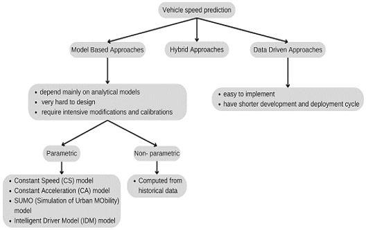
Researchers have been consistently investigating the prediction of vehicle speed, broadly classifying methodologies into three primary categories: model- based, data-driven, and hybrid techniques [8]. Model-based techniques mainly rely on analytical models, which present design challenges because they require extensive adjustments and calibrations for practical situations. On the other hand, data-driven strategies have shorter development cycles and are simpler to apply [9]. The goal of hybrid approaches is to combine data-driven and model- based techniques [10].
There are two further categories of model-based approaches: parametric and non-parametric. For accuracy, parametric approaches require large amounts of representative training data and assume the structure of the prediction model. Constant Acceleration (CA), Constant Speed (CS), the Simulation of Urban Mobility (SUMO) model, and the Intelligent Driver Model (IDM) are a few examples [11]. However, non-parametric techniques can be calculated from historical data and do not require pre-fixing of the model structure, as demonstrated in Figure 1. The study [12] uses 10-fold cross-validation for different prediction horizons and assessed six models using parametric and non- parametric methods. The findings showed that while advanced parametric models show higher accuracy in long-term forecasting, parametric models perform best in short-term prediction.
Figure 1. Vehicle speed prediction approaches
In terms of EV or non-EV vehicle speed predictions, numerous works using deep learning have been proposed. Recent studies have leveraged deep learning for vehicle speed prediction using diverse models and data sources. A DNN-based approach using shared EV data from Beijing showed effective short-term speed forecasting with an RMSE of 1.53 [13]. Another study to predict vehicle speed was based on Adaptive neuro fuzzy inference system (ANFIS). The approach outperforming traditional methods with an RMSE of 7.73 mph [14]. The proposed Long Short-Term Memory (LSTM) based speed prediction model in the study [15] demonstrated an average RMSE of 1.797 km/h along the prediction horizon, significantly outperforming the Artificial Neural Network (ANN) which recorded an RMSE of 7.012 km/h. During hyperparameter optimization, the best model achieved an average RMSE of 4.753 km/h on the validation data. Across six distinct driving tests, the LSTM model yielded an average RMSE of 5.023 km/h, with individual test results ranging from 4.030 km/h to 5.820 km/h.
A hybrid BP-LSTM model improved long-term predictions across different road types, with RMSE values ranging from 5.78 to 10.92 [16]. This model was also integrated into an energy management strategy for PHEVs, reducing fuel use by 4.97% and achieving an RMSE of 1.84 m/s [17]. Other efforts include speed prediction under varying road statuses using linear regression and DBN with up to 95% accuracy [18]. In the study [19], a Deep Belief Network model was proposed to predict electric vehicle driveline speed ratios. It achieving an R2 value of 0.9989, alongside a minimal Mean Squared Error (MSE) of 0.01 and a Mean Absolute Percentage Error (MAPE) of 0.0008%, the model significantly enhances the efficiency and reliability of vehicle design processes. Another real-time forecasting for EVs on urban roads was also proposed in which Twizy vehicle data was used and it showed that LSTM outperformed Auto Regressive Integrated Moving Average (ARIMA), CNN, and ConvLSTM [7].
Another related work focusing on the implementation of Deep Belief Network (DBN) to predict the EV speed [20]. The proposed model managed to obtain very low prediction errors (as low as 0.001%). The work also produced high R2 values in the experiments.
In the study [21], a hierarchical LSTM-based vehicle trajectory prediction model was introduced that determines driving intention prediction, lane change time estimation, and interaction information from surrounding vehicles. Tested on the NGSIM dataset, the model achieved superior performance in medium- to long-term prediction horizons. Specifically, at a 5-second forecast horizon, the lateral RMSE was reduced to 0.46 m (a 70% improvement over the Constant Acceleration model and 25% over the S_LSTM model), while the longitudinal RMSE dropped to 4.53 m, marking a 52% and 20% reduction respectively.
Recent studies highlight the effectiveness of deep learning models, particularly LSTM networks for vehicle speed prediction in both short and long-term scenarios. Models integrating LSTM with other techniques, such as Backpropagation or adaptive control, have shown improved accuracy by capturing temporal dependencies and complex driving patterns. While deep models excel in nonlinear pattern recognition, statistical methods like ARIMA are known for modeling linear trends effectively. However, few works have explored the synergy between these two approaches. Therefore, a hybrid model combining LSTM and ARIMA holds strong potential to leverage both temporal pattern recognition and linear trend modeling, offering a more robust and accurate solution for vehicle speed prediction. This integration is particularly valuable for real-time applications and energy-efficient vehicle control strategies.
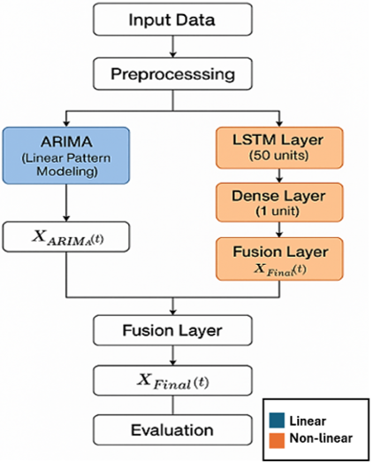
The implementation of the proposed hybrid LSTM model for EV speed prediction begins with the preparation of the programming environment by importing the necessary libraries. These include Pandas and NumPy for data manipulation, TensorFlow and Keras for deep learning model development, and MinMaxScaler from Scikit-learn for data normalization. In addition, evaluation metrics such as mean squared error (MSE) and R-squared (R²) are imported to assess model performance. A random seed is also set to ensure the reproducibility of the results throughout the experimentation. The architecture of the proposed LSTM and ARIMA is shown in Figure 2.
The dataset, which consists of time series telemetry data related to electric vehicle movement, is then loaded into memory. This dataset includes key features such as speed, mode, weather conditions, and trajectory-related attributes. Prior to model training, several preprocessing steps are performed. Categorical data such as driving mode and weather conditions are encoded into numerical values. The speed variable, which serves as the prediction target, is scaled to a normalized range between 0 and 1 using the MinMaxScaler method. This scaling ensures that the LSTM model receives inputs within a consistent range, facilitating better convergence during training. After prediction, the outputs were inverse-transformed using the same scaler to restore the predicted speed values to their original scale for evaluation and interpretability. Furthermore, to capture more granular patterns, the dataset is segmented into smaller trajectory segments based on logical or spatial criteria.
Following preprocessing, the data is prepared for LSTM input by applying a sliding window technique. Historical sequences of 5- or 10-time steps are used as input features, while the model is tasked with forecasting the speed 30 or 60 time steps ahead. The data is then divided into training and testing sets using an 80:20 ratio to facilitate model learning and performance evaluation on unseen data.
For model development, a sequential LSTM architecture is constructed, consisting of a single LSTM layer with 50 memory units, followed by a dense output layer with one neuron for continuous speed prediction. The model is compiled using the mean squared error loss function and the Adam optimizer, which is well-suited for handling noisy time series data.
The input sequences are converted into TensorFlow datasets, shuffled using a buffer size equal to the dataset length to ensure uniform randomness, and batched with a size of 1024 for efficient training. The model is trained for 500 epochs, allowing it to learn both short and long-term temporal dependencies in the data.
Once training is completed, the model is used to generate predictions on the test data. These predicted speed values are then rescaled back to their original scale for interpretability. To evaluate the model’s predictive performance, metrics such as Symmetric Mean Absolute Percentage Error (SMAPE), Root Mean Squared Error (RMSE), and R-squared (R²) are calculated. The results are visualized by plotting actual versus predicted speed values, providing a clear depiction of how well the model tracks the speed trajectory over time, both for the full dataset and for individual segments, as illustrated in Figure 3.
Figure 3. LSTM-ARIMA model flow
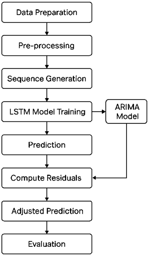
Building on the LSTM model, a hybrid approach combining LSTM and ARIMA is proposed to further enhance the prediction accuracy of EV speed. As illustrated in Figure 3, which depicts the LSTM-ARIMA implementation for both whole and segmented trajectories, the initial phases of the workflow comprising data preparation, pre-processing, sequence generation, model training, and evaluation—follow the same procedures as those employed in the standalone LSTM model. However, the hybrid model introduces additional steps to incorporate residual modeling using the ARIMA technique.
After obtaining the initial predictions from the LSTM model, the residuals are computed by subtracting the predicted speed values from the actual observed values. These residuals represent the error terms, or the components not captured by the LSTM, particularly any remaining linear structures or short-term fluctuations in the data.
To model these residuals, an ARIMA model with parameters (1,1,1) is fitted to the residual time series. This was selected based on preliminary residual diagnostics, including the autocorrelation function (ACF) and partial autocorrelation function (PACF) plots, which indicated significant lag-1 autocorrelation and a need for first-order differencing to achieve stationarity.
The ARIMA model then generates predictions for the residuals over the forecast horizon. These predicted residuals are added to the scaled LSTM predictions to adjust and refine the forecast. The adjusted predictions are then inverse-transformed using the same scaler previously applied to the target variable, restoring them to their original scale for evaluation and comparison.
The performance of the hybrid LSTM-ARIMA model is then evaluated using standard metrics: SMAPE, RMSE, and R-squared (R²). These metrics are recalculated based on the adjusted predictions to assess the improvement achieved by the hybridization. Visualization of the predicted versus actual speed values further illustrates the model's effectiveness in capturing both the nonlinear dynamics (through LSTM) and the remaining linear patterns (through ARIMA), offering a more comprehensive and accurate prediction of electric vehicle speed trajectories.
3.1 Datasets
The dataset employed in this study is derived from a previously published work titled Embedded Real-Time Speed Forecasting for Electric Vehicles: A Case Study on RSK Urban Roads [7]. The data collection was conducted using the Renault Twizy, a compact fully electric vehicle with a maximum speed of 80 km/h. The dataset captures detailed driving behavior and vehicle telemetry across various urban environments and time periods, making it well-suited for developing and evaluating time-series prediction models.
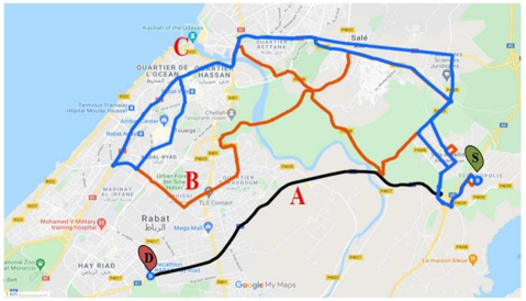
To reflect diverse traffic patterns and road conditions, the experiments were carried out along three distinct urban routes—Trajectory A, Trajectory B, and Trajectory C—located in the Sala Al Jadida and Rabat regions of Morocco, as illustrated in Figure 4. Each route varies in duration, ranging from approximately 30 minutes to 2 hours, and was driven multiple times across different times of day, including morning, noon, and afternoon sessions. This repetition provides a rich temporal variation that enhances the dataset's robustness and generalizability.
Data acquisition was facilitated by an NVIDIA Jetson Nano computing platform paired with a transceiver. Measurements were recorded at multiple sampling intervals, specifically at 1-second (TM1), 5-second (TM5), and 10-second (TM10) time steps, allowing for analysis at varying temporal resolutions. The collected data includes variables such as vehicle speed, mode of operation, and weather conditions, forming a comprehensive dataset suitable for training and evaluating deep learning and hybrid time-series models for electric vehicle speed forecasting.
Figure 4. Trajectory A, B and C from the dataset
The experiments of the proposed LSTM-ARIMA hybrid model for speed prediction were done on three trajectory types of trajectories (A, B, C), whole trajectory, segment trajectory, steps (5 and 10), and forecast horizon (30 and 60). The results of the proposed work are compared with benchmark LSTM model for the case of numerical sequences. The results shown will be based on the metrics used which are SMAPE, RMSE and R² for whole trajectory and segmented trajectory.
4.1 Whole trajectory
In terms of the SMAPE metric for the whole trajectory experiments the results are shown in Table 1. For Trajectory A with a collected step of 5 and a forecast horizon of 30 steps, the LSTM model yields a SMAPE of 21.00%, while the LSTM-ARIMA hybrid model trained with 500 epochs improves the result to 19.23%. At a 60-step forecast horizon, the LSTM model achieves a SMAPE of 19.66%, whereas the LSTM-ARIMA model records a slightly higher SMAPE of 21.08%. When the collected step increases to 10, the SMAPE for the LSTM model is 17.93% at 30 steps, while LSTM-ARIMA further reduces this to 15.97%. For a 60-step horizon, the LSTM model yields 16.93%, with the LSTM-ARIMA showing a moderate increase to 20.09%.
Table 1. Symmetric Mean Absolute Percentage Error (SMAPE) results for whole trajectory data
|
Trajectory |
Collected Step |
Forecast Horizon |
SMAPE |
|
|
Epoch |
LSTM |
LSTM-ARIMA |
||
|
500 |
500 |
|||
|
A |
5 |
30 |
21.00 |
19.23 |
|
60 |
19.66 |
21.08 |
||
|
10 |
30 |
17.93 |
15.97 |
|
|
60 |
16.93 |
20.09 |
||
|
B |
5 |
30 |
57.79 |
57.31 |
|
60 |
61.55 |
58.75 |
||
|
10 |
30 |
52.66 |
50.01 |
|
|
60 |
52.39 |
52.04 |
||
|
C |
5 |
30 |
80.83 |
79.67 |
|
60 |
73.31 |
74.25 |
||
|
10 |
30 |
73.53 |
71.87 |
|
|
60 |
70.56 |
72.76 |
||
In the case of Trajectory B, the performance gains from the hybrid model are more modest. With a collected step of 5 and a forecast horizon of 30 steps, the LSTM model achieves a SMAPE of 57.79%, and LSTM-ARIMA slightly reduces it to 57.31%. For the 60-step forecast, the SMAPE improves from 61.55% (LSTM) to 58.75% (LSTM-ARIMA). With a collected step of 10, LSTM achieves a SMAPE of 52.66% at 30 steps, and LSTM-ARIMA reduces this to 50.01%. For the 60-step forecast, the LSTM model records 52.39%, while LSTM-ARIMA marginally improves it to 52.04%.
For Trajectory C, with a collected step of 5 and a 30-step forecast horizon, the LSTM model produces a SMAPE of 80.83%, and LSTM-ARIMA slightly improves this to 79.67%. At 60 steps, the SMAPE increases from 73.31% (LSTM) to 74.25% (LSTM-ARIMA). When the collected step is 10, the LSTM model yields a SMAPE of 73.53% for 30-step forecasts, with LSTM-ARIMA reducing it to 71.87%. For a 60-step horizon, the LSTM model records 70.56%, while LSTM-ARIMA shows a slight increase to 72.76%.
In terms of Symmetric Mean Absolute Percentage Error (SMAPE) in whole trajectory setup, the proposed LSTM–ARIMA hybrid model generally demonstrates improved accuracy over the baseline LSTM, particularly for shorter forecast horizons and higher collected steps. For Trajectory A, the hybrid model significantly reduces SMAPE at 30-step forecasts for both collected steps of 5 and 10, confirming its effectiveness in correcting short-term errors. However, for the 60-step forecasts, the LSTM-ARIMA model occasionally yields slightly higher SMAPE values, indicating limited benefit from residual modeling over longer horizons.
In Trajectory B, improvements from the hybrid approach are modest but consistent, especially at 60-step forecasts, where SMAPE is reduced more noticeably. This reflects ARIMA’s strength in capturing residual linear patterns that LSTM may overlook.
For Trajectory C, which exhibits higher prediction difficulty as reflected by overall higher SMAPE values, the LSTM–ARIMA model provides only slight improvements in most cases, with occasional performance drops for longer forecast horizons. This suggests that while the hybrid model offers enhancements in SMAPE, its effectiveness varies depending on the trajectory complexity and temporal resolution. Overall, hybridization offers measurable but context-dependent gains in predictive accuracy.
In terms of RMSE for whole trajectory experiments, the results are shown in Table 2. For Trajectory A with a collected step of 5, the LSTM model records an RMSE of 8.69 for a 30-step forecast horizon, whereas the proposed LSTM–ARIMA hybrid model achieves a lower RMSE of 7.33 at 500 epochs. For the 60-step forecast horizon, the LSTM outperforms the hybrid with an RMSE of 7.25 compared to 9.44 from the LSTM–ARIMA model. When the collected step is increased to 10, the LSTM model yields an RMSE of 5.96 for the 30-step horizon, while the hybrid improves performance with an RMSE of 5.25. For the 60-step horizon, the LSTM achieves 5.47, whereas the LSTM–ARIMA gives 7.00.
Table 2. RMSE results for whole trajectory data
|
Trajectory |
Collected Step |
Forecast Horizon |
RMSE |
|
|
Epoch |
LSTM |
LSTM-ARIMA |
||
|
500 |
500 |
|||
|
A |
5 |
30 |
08.69 |
07.33 |
|
60 |
07.25 |
09.44 |
||
|
10 |
30 |
05.96 |
05.25 |
|
|
60 |
05.47 |
07.00 |
||
|
B |
5 |
30 |
10.21 |
10.22 |
|
60 |
11.98 |
10.49 |
||
|
10 |
30 |
07.62 |
07.06 |
|
|
60 |
08.27 |
08.20 |
||
|
C |
5 |
30 |
11.00 |
10.88 |
|
60 |
09.37 |
09.62 |
||
|
10 |
30 |
08.22 |
07.96 |
|
|
60 |
07.43 |
07.67 |
||
For Trajectory B, with a collected step of 5, the LSTM model produces an RMSE of 10.21 for the 30-step forecast horizon, while the LSTM–ARIMA hybrid model at 500 epochs yields a nearly identical RMSE of 10.22. However, for the 60-step horizon, the hybrid model improves upon the LSTM's RMSE of 11.98 by achieving 10.49. When the collected step is increased to 10, the LSTM model records an RMSE of 7.62 for the 30-step horizon, with the LSTM–ARIMA reducing it further to 7.06. For the 60-step forecast, the LSTM model attains an RMSE of 8.27, and the hybrid model shows a slight improvement with 8.20.
For Trajectory C, the LSTM-ARIMA hybrid model showed slight improvements in RMSE performance over the baseline LSTM model at most configurations. With a collected step of 5 and a 30-step forecast horizon, the LSTM model yielded an RMSE of 11.00, while the LSTM-ARIMA model reduced this to 10.88. For a 60-step forecast horizon, the LSTM model achieved a lower RMSE of 9.37, although the hybrid model recorded a slightly higher RMSE of 9.62.
When the collected step increased to 10, the hybrid model continued to show modest gains. For the 30-step forecast horizon, the LSTM model recorded an RMSE of 8.22, while LSTM-ARIMA improved this to 7.96. At the 60-step horizon, the LSTM model achieved an RMSE of 7.43, with the LSTM-ARIMA model showing a marginal increase to 7.67.
In terms of Root Mean Squared Error (RMSE), the LSTM–ARIMA hybrid model demonstrates consistent improvements over the standalone LSTM model in several configurations, particularly for shorter forecast horizons and higher collected steps. Notably, in Trajectories A and B, the hybrid model outperforms LSTM when the collected step is 10, indicating better short-term error correction. However, for longer forecast horizons—especially in Trajectories A and C—the hybrid model occasionally underperforms compared to LSTM, suggesting that ARIMA's residual correction is more effective in scenarios with stronger short-term dependencies. Overall, the hybrid approach enhances prediction accuracy in most settings, validating its suitability for electric vehicle speed forecasting where capturing both linear and nonlinear patterns is critical.
In terms of coefficient of determination (R²), the LSTM-ARIMA hybrid model generally outperformed the standalone LSTM model across various configurations and trajectories, indicating improved explanatory power in modeling electric vehicle speed. The full results of R² for the Whole Trajectory experiments are shown in Table 3.
Table 3. R² results for whole trajectory data
|
Trajectory |
Collected Step |
Forecast Horizon |
R2 |
|
|
Epoch |
LSTM |
LSTM-ARIMA |
||
|
500 |
500 |
|||
|
A |
5 |
30 |
82.16 |
87.31 |
|
60 |
86.61 |
77.27 |
||
|
10 |
30 |
91.50 |
93.40 |
|
|
60 |
92.34 |
87.48 |
||
|
B |
5 |
30 |
66.92 |
68.85 |
|
60 |
54.31 |
65.00 |
||
|
10 |
30 |
81.59 |
84.18 |
|
|
60 |
78.22 |
78.57 |
||
|
C |
5 |
30 |
71.29 |
71.96 |
|
60 |
79.24 |
78.14 |
||
|
10 |
30 |
84.01 |
85.00 |
|
|
60 |
86.98 |
86.11 |
||
For Trajectory A, with a collected step of 5 and a 30-step forecast horizon, the LSTM model attained an R² of 82.16%, which was further improved by the LSTM-ARIMA model to 87.31%. However, for the 60-step forecast horizon, the LSTM model yielded an R² of 86.61%, while the hybrid model showed a slight reduction to 77.27%, suggesting that the integration may be less effective for longer horizons under this configuration. When the collected step increased to 10, both models showed higher performance: the LSTM model achieved 91.50% R² for the 30-step forecast, and the LSTM-ARIMA model enhanced it further to 93.40%. For the 60-step forecast, the LSTM model reached 92.34%, while the hybrid model recorded a slightly lower R² of 87.48%.
For Trajectory B, with a collected step of 5, the LSTM model registered an R² of 66.92% for a 30-step forecast horizon. The LSTM-ARIMA model improved this marginally to 68.85%. At a 60-step forecast, the LSTM model achieved an R² of 54.31%, and the hybrid model demonstrated a substantial improvement, reaching 65.00%. With a collected step of 10, the LSTM model achieved an R² of 81.59% for the 30-step forecast, while the LSTM-ARIMA model further improved this to 84.18%. For the 60-step forecast, both models performed similarly, with the LSTM at 78.22% and the hybrid model slightly better at 78.57%.
For Trajectory C, performance differences between the two models were less pronounced. With a collected step of 5 and a 30-step forecast horizon, the LSTM model recorded an R² of 71.29%, while the LSTM-ARIMA model showed a modest improvement to 71.96%. At a 60-step forecast, the LSTM model reached 79.24%, while the hybrid model slightly decreased to 78.14%. When the collected step was increased to 10, the LSTM model attained an R² of 84.01% for the 30-step horizon, with the hybrid model improving this to 85.00%. For the 60-step forecast, the LSTM model scored 86.98%, and the LSTM-ARIMA model followed closely with 86.11%.
These results indicate that the hybrid LSTM-ARIMA approach can effectively enhance the prediction accuracy in most scenarios, particularly for shorter forecast horizons and smaller input step sizes. However, the performance gains diminish or slightly regress when applied to longer horizons or more stable patterns, particularly in Trajectories A and C. This suggests that while ARIMA enhances the residual correction capability of LSTM, its contribution becomes limited when long-range temporal dependencies dominate the forecast window.
4.2 Segmented Trajectory
As shown in Table 4, for Trajectory A at 500 epochs and a collected step size of 5, the LSTM model yields a SMAPE of 12.73% for the 30-step forecast horizon, which is notably improved to 6.11% by the LSTM–ARIMA hybrid model. For the 60-step forecast, the LSTM model records a SMAPE of 12.95%, while the hybrid model reduces it to 6.89%. When the collected step size is increased to 10, the LSTM model produces a SMAPE of 28.51% for the 30-step forecast, whereas the LSTM–ARIMA model achieves a significantly lower SMAPE of 5.51%. For the 60-step horizon, the LSTM model's SMAPE of 11.81% is reduced to 8.46% by the hybrid approach.
Table 4. SMAPE results for segmented trajectory data
|
Trajectory |
Collected Step |
Forecast Horizon |
SMAPE |
|
|
Epoch |
LSTM |
LSTM-ARIMA |
||
|
500 |
500 |
|||
|
A |
5 |
30 |
12.73 |
06.11 |
|
60 |
12.95 |
06.89 |
||
|
10 |
30 |
28.51 |
05.51 |
|
|
60 |
11.81 |
08.46 |
||
|
B |
5 |
30 |
50.81 |
31.14 |
|
60 |
49.55 |
31.35 |
||
|
10 |
30 |
44.99 |
30.74 |
|
|
60 |
46.38 |
31.09 |
||
|
C |
5 |
30 |
76.49 |
60.08 |
|
60 |
75.86 |
59.97 |
||
|
10 |
30 |
73.00 |
59.14 |
|
|
60 |
71.14 |
59.18 |
||
In Trajectory B, using a collected step size of 5, the LSTM model attains a SMAPE of 50.81% for the 30-step forecast horizon, while the LSTM–ARIMA model reduces it to 31.14%. For the 60-step forecast, the LSTM model's SMAPE of 49.55% improved to 31.35% by the hybrid model. When the collected step is increased to 10, the LSTM model yields a SMAPE of 44.99% for the 30-step forecast, with the hybrid model reducing it to 31.09%. For the 60-step forecast horizon, the LSTM model records a SMAPE of 46.38%, which is likewise reduced to 31.09% through the hybrid method.
For Trajectory C, with a collected step size of 5, the LSTM model shows a SMAPE of 76.49% for the 30-step forecast, which is improved to 60.08% by the LSTM–ARIMA model. For the 60-step horizon, the SMAPE decreases from 75.86% (LSTM) to 59.97% (hybrid). When the collected step size is increased to 10, the LSTM model records a SMAPE of 73.00% for the 30-step forecast, while the hybrid model achieves a lower SMAPE of 59.14%. For the 60-step horizon, the LSTM model's SMAPE of 71.14% is further reduced to 59.18% by the hybrid model.
As presented in Table 5, for Trajectory A at 500 training epochs and a collected step size of 5, the LSTM model achieves an RMSE of 3.74 for a 30-step forecast horizon. The proposed LSTM–ARIMA hybrid model substantially reduces the error to 0.64. For the 60-step horizon, the RMSE of the LSTM model is 3.37, which is again markedly improved by the hybrid model to 0.72. When the collected step size is increased to 10, the LSTM model records an RMSE of 4.63 for the 30-step forecast, while the hybrid model reduces it to 0.58. Similarly, for the 60-step horizon, the LSTM model yields an RMSE of 2.51, with the LSTM–ARIMA model improving the result to 0.58.
Table 5. RMSE results for segmented trajectory data
|
Trajectory |
Collected Step |
Forecast Horizon |
RMSE |
|
|
Epoch |
LSTM |
LSTM-ARIMA |
||
|
500 |
500 |
|||
|
A |
5 |
30 |
03.74 |
00.64 |
|
60 |
03.37 |
00.72 |
||
|
10 |
30 |
04.63 |
00.58 |
|
|
60 |
02.51 |
00.58 |
||
|
B |
5 |
30 |
07.11 |
00.87 |
|
60 |
06.30 |
00.92 |
||
|
10 |
30 |
05.39 |
00.86 |
|
|
60 |
05.80 |
00.84 |
||
|
C |
5 |
30 |
07.52 |
01.02 |
|
60 |
06.59 |
00.97 |
||
|
10 |
30 |
06.55 |
00.87 |
|
|
60 |
05.46 |
00.77 |
||
For Trajectory B, using a collected step size of 5, the LSTM model produces an RMSE of 7.11 for the 30-step horizon, whereas the LSTM–ARIMA hybrid model lowers the error significantly to 0.87. For the 60-step forecast, the LSTM model records an RMSE of 6.30, which is reduced to 0.92 by the hybrid approach. With a collected step size of 10, the LSTM model attains an RMSE of 4.95 for the 30-step forecast, while the hybrid model achieves a reduced RMSE of 0.86. For the 60-step horizon, the LSTM model's RMSE of 5.80 is improved to 0.84 by the hybrid model.
In the case of Trajectory C, with a collected step size of 5, the LSTM model registers an RMSE of 7.52 for the 30-step forecast, which is significantly decreased to 1.02 by the LSTM–ARIMA model. For the 60-step horizon, the RMSE is reduced from 6.59 to 0.99. When the collected step size is set to 10, the LSTM model records an RMSE of 6.55 for the 30-step forecast, while the hybrid model further reduces it to 0.87. For the 60-step forecast, the LSTM model yields an RMSE of 5.46, which is improved to 0.77 through the hybrid model.
As detailed in Table 6, for Trajectory A at 500 epochs and a collected step size of 5, the LSTM model achieves an R² of 96.81% for the 30-step forecast horizon, which is enhanced to 99.91% by the LSTM–ARIMA hybrid model. For the 60-step forecast, the LSTM model records an R² of 97.32%, while the hybrid model further improves it to 99.88%. When the collected step size is increased to 10, the LSTM model attains an R² of 96.77% for the 30-step forecast, and the hybrid model increases this to 99.92%. For the 60-step horizon, the R² improves from 98.52% (LSTM) to 99.92% (hybrid).
Table 6. R² results for segmented trajectory data
|
Trajectory |
Collected Step |
Forecast Horizon |
R2 |
|
|
Epoch |
LSTM |
LSTM-ARIMA |
||
|
500 |
500 |
|||
|
A |
5 |
30 |
96.81 |
99.91 |
|
60 |
97.32 |
99.88 |
||
|
10 |
30 |
96.77 |
99.92 |
|
|
60 |
98.52 |
99.92 |
||
|
B |
5 |
30 |
84.08 |
99.76 |
|
60 |
87.50 |
99.73 |
||
|
10 |
30 |
90.86 |
99.77 |
|
|
60 |
89.36 |
99.78 |
||
|
C |
5 |
30 |
86.25 |
99.75 |
|
60 |
89.50 |
99.77 |
||
|
10 |
30 |
89.58 |
99.81 |
|
|
60 |
92.77 |
99.86 |
||
In Trajectory B, with a collected step size of 5, the LSTM model produces an R² of 84.08% for the 30-step forecast, while the LSTM–ARIMA model markedly improves this to 99.76%. For the 60-step horizon, the LSTM model records an R² of 87.50%, which is enhanced to 99.73% by the hybrid model. With a collected step size of 10, the LSTM model yields an R² of 90.80% for the 30-step forecast, and the hybrid model improves it to 99.78%. For the 60-step horizon, the R² increases from 89.36% to 99.78% through the hybrid approach.
For Trajectory C, using a collected step size of 5, the LSTM model achieves an R² of 86.25% for the 30-step forecast horizon, which is significantly improved to 99.75% by the LSTM–ARIMA model. For the 60-step forecast, the LSTM model yields an R² of 89.50%, with the hybrid model raising it to 99.74%. When the collected step is set to 10, the LSTM model attains an R² of 89.58% for the 30-step horizon, while the hybrid model achieves a higher R² of 99.81%. For the 60-step forecast, the LSTM model’s R² of 92.77% is further enhanced to 99.86% by the hybrid approach.
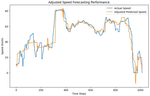
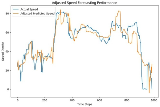
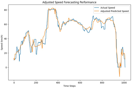
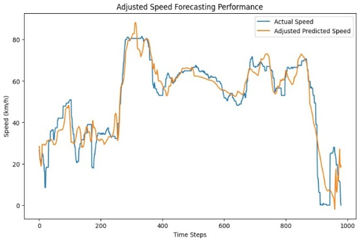
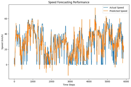
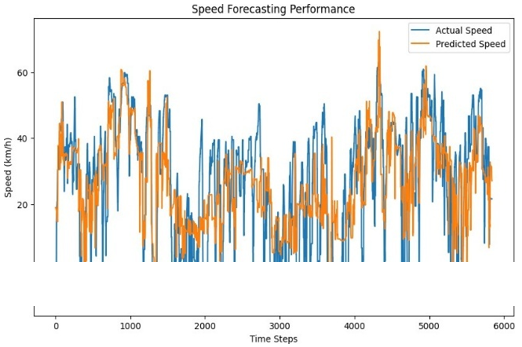
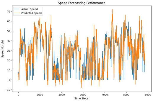
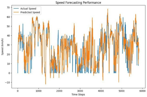
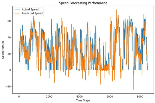
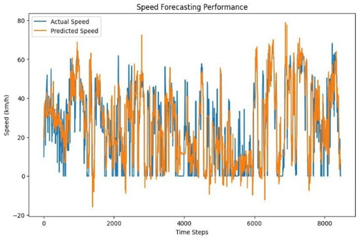
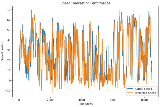
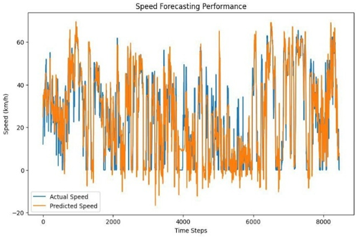
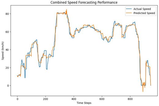
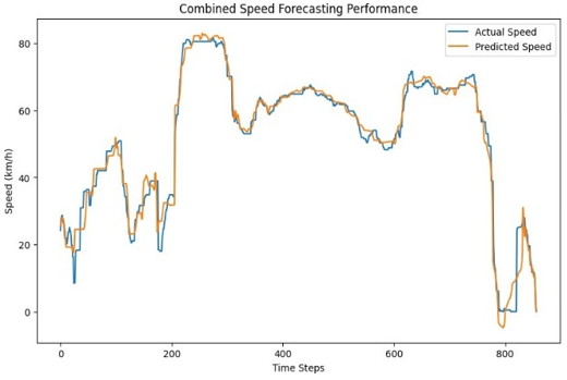
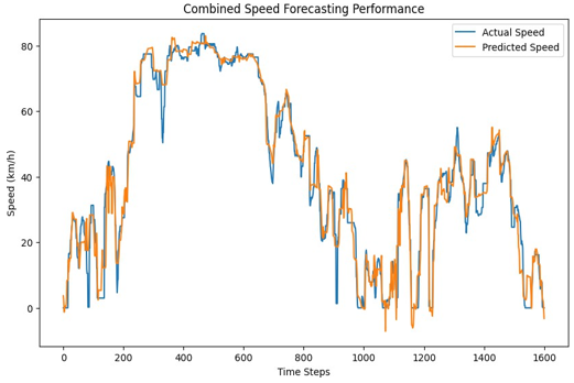
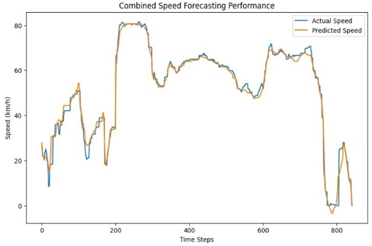
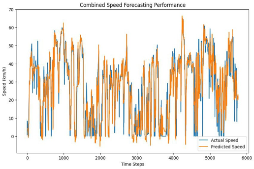
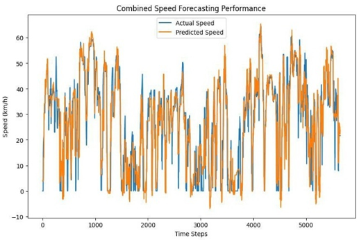
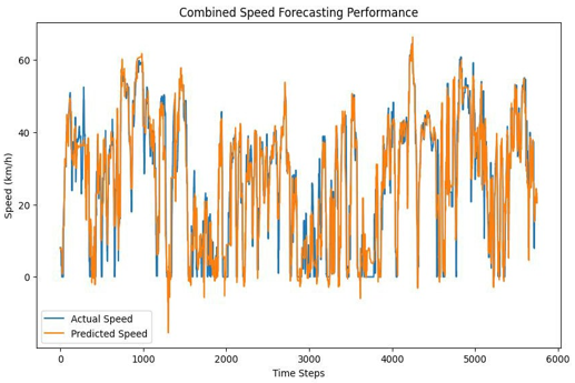
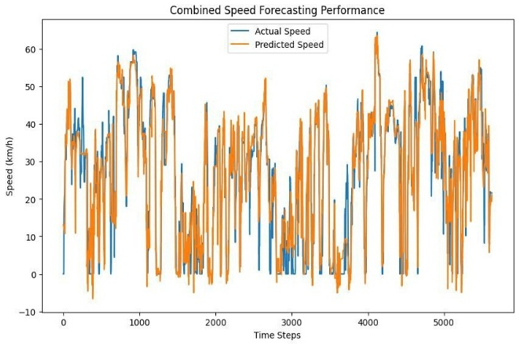
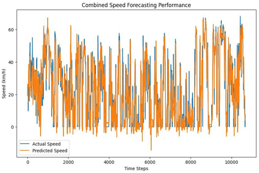
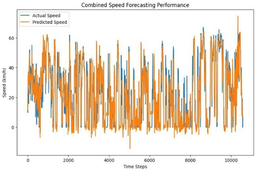
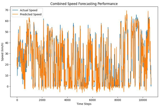
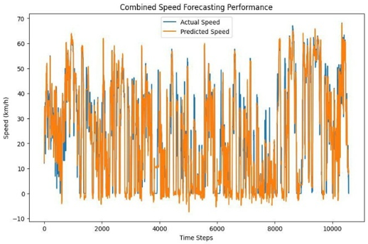
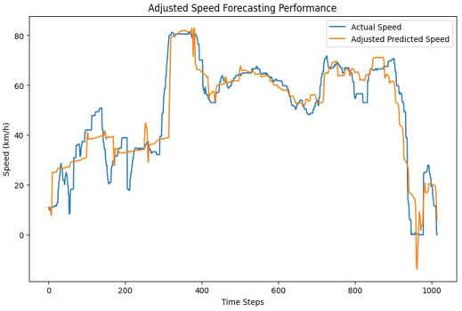
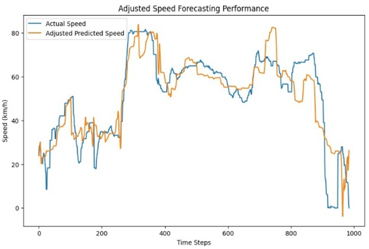
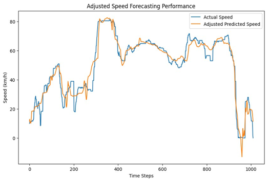
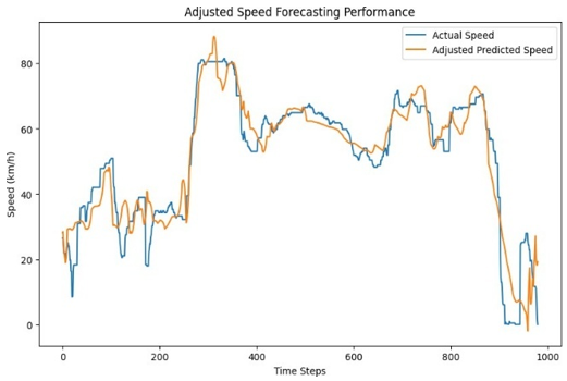
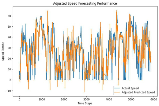
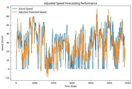
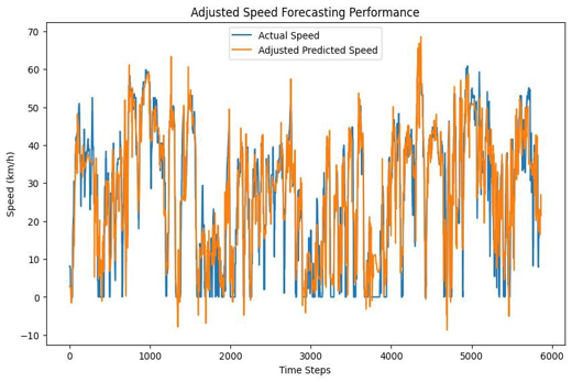
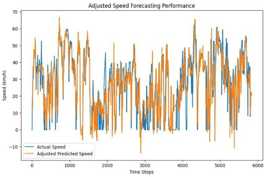
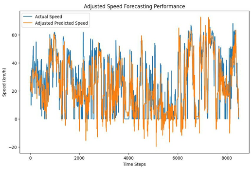
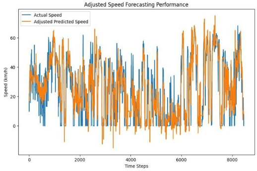
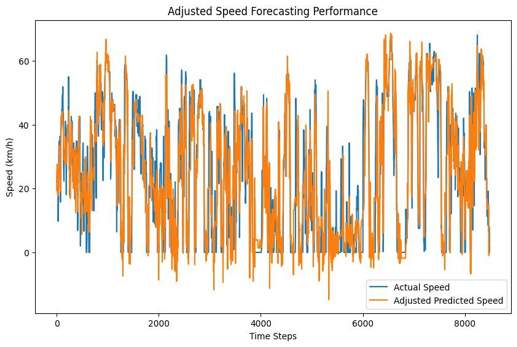
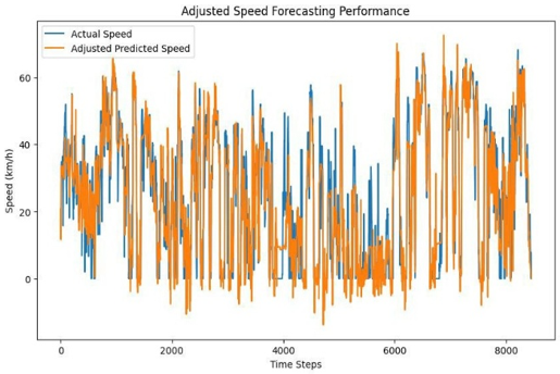
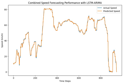
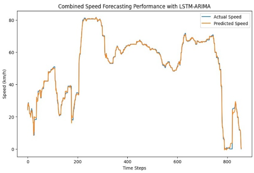
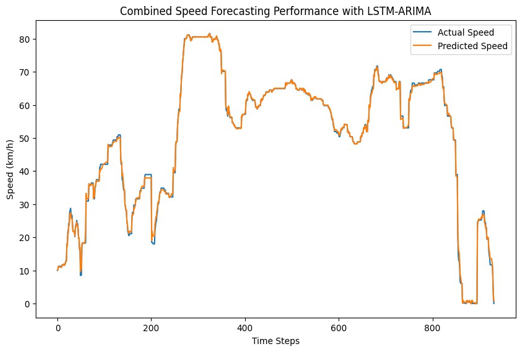
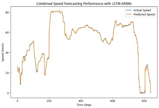
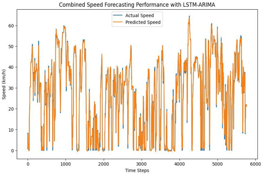
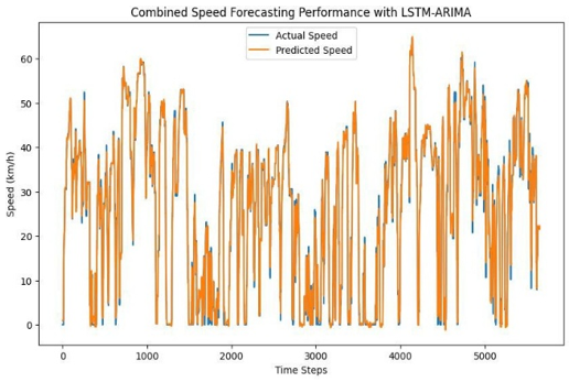
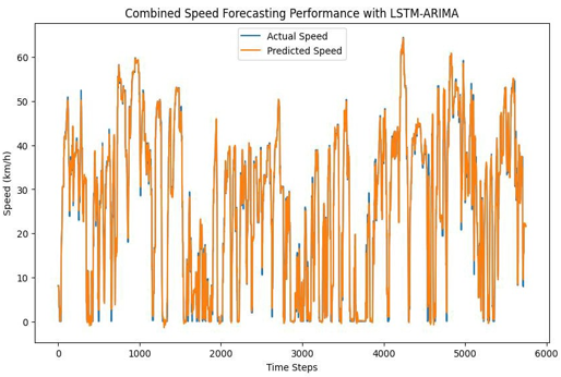
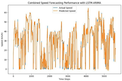
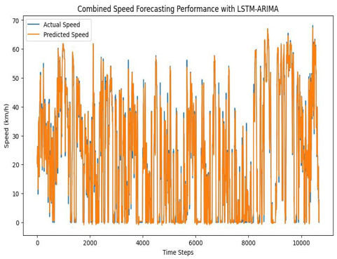
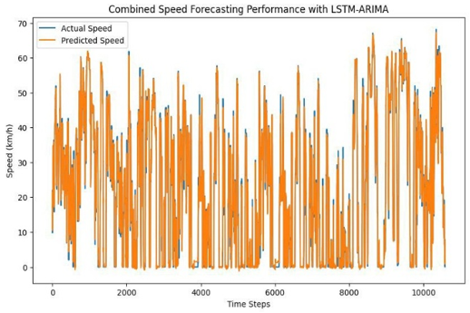
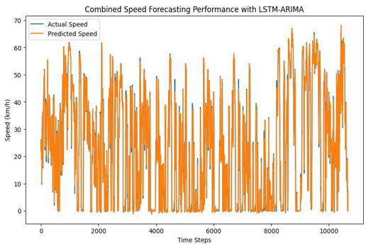
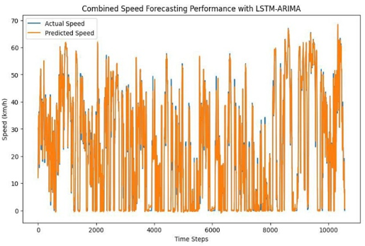
The corresponding predicted versus actual speed plots that support the findings discussed in this section are provided in the Appendix for reference. Figures A1 to A12 present the prediction results of the LSTM model applied to the full trajectory, while Figures A13 to A24 illustrate its performance on segmented trajectories. The prediction outcomes of the hybrid LSTM-ARIMA model on the full trajectory are shown in Figures A25 to A36, and Figures A37 to A48 depict the hybrid model’s performance on segmented trajectories. These figures offer a comprehensive visual representation of the model outputs across different scenarios and further reinforce the quantitative results presented above.
Based on the experimental results across all segmented trajectories (A, B, and C), the LSTM–ARIMA hybrid approach consistently outperforms the standalone LSTM model in terms of RMSE, SMAPE, and R² metrics. The hybrid model demonstrates significantly lower forecast errors and higher predictive accuracy across varying forecast horizons (30-step and 60-step) and collected step sizes (5 and 10). These improvements are particularly pronounced in more complex or variable trajectories, such as Trajectory B and C, indicating the robustness and generalizability of the LSTM–ARIMA model in handling diverse motion patterns. Overall, the findings confirm that integrating ARIMA with LSTM enhances the model’s capability to capture both linear and nonlinear temporal dependencies in segmented trajectory prediction tasks.
The experimental findings confirm that the proposed LSTM–ARIMA hybrid model enhances prediction accuracy across various trajectory types, outperforming the baseline LSTM in most settings.
In whole trajectory experiments, the hybrid approach achieved notable reductions in SMAPE and RMSE, especially for shorter forecast horizons and higher collected steps, with consistent improvements in R². While performance gains diminished for longer horizons, particularly in Trajectories A and C, the hybrid model still demonstrated effective residual correction.
In segmented trajectory experiments, the hybrid model delivered significant performance boosts, with RMSE reductions exceeding 80% and R² values approaching or surpassing 99% across all configurations. These results highlight the hybrid model’s strength in capturing both nonlinear and linear temporal dynamics, particularly in complex or variable motion patterns, making it a robust and effective solution for electric vehicle speed forecasting.
Overall, the hybrid model demonstrated superior accuracy in scenarios involving shorter input sequences and shorter forecast horizons, suggesting that the ARIMA component is effective at capturing short-term temporal dependencies. Meanwhile, the LSTM component retained its strength in modeling long-term, non-linear patterns. The integration of these two approaches, which include statistical and neural network-based resulted in a robust, comprehensive, and efficient predictive framework. The model achieved satisfactory levels of accuracy and responsiveness, making it a promising solution for real-time electric vehicle speed forecasting applications.
Future work can be further explored and expanded in terms of integrating with more advanced deep learning architectures, for example, such as hybrid Transformer-based models and other similar structures, so as to enhance the overall capability of capturing long-term temporal dependencies in EV speed prediction tasks. Additionally, the development and implementation of end-to-end deployment pipelines, which may include real-time inference support and cloud-based modeling solutions, would greatly facilitate practical implementation within modern intelligent transportation systems. To better support deployment in resource-constrained devices and embedded platforms, various model compression and lightweight optimization techniques—such as pruning, quantization, or knowledge distillation, among others—should also be actively explored and considered.
The authors would like to express their sincere appreciation to the Faculty of Computer Science and Information Technology, Universiti Putra Malaysia, for the invaluable support, research facilities, and financial assistance provided throughout the course of this study.
Figure A1. Whole Trajectory LSTM-ARIMA, Trajectory A, Collection Step 5, Forecast Horizon 30 and Epoch 500
Figure A2. Whole Trajectory LSTM-ARIMA, Trajectory A, Collection Step 5, Forecast Horizon 60 and Epoch 500
Figure A3. Whole Trajectory LSTM-ARIMA, Trajectory A, Collection Step 10, Forecast Horizon 30 and Epoch
Figure A4. Whole Trajectory LSTM-ARIMA, Trajectory A, Collection Step 10, Forecast Horizon 60 and Epoch 500
Figure A5. Whole Trajectory LSTM-ARIMA, Trajectory B, Collection Step 5, Forecast Horizon 30 and Epoch 500
Figure A6. Whole Trajectory LSTM-ARIMA, Trajectory B, Collection Step 5, Forecast Horizon 60 and Epoch 500
Figure A7. Whole Trajectory LSTM-ARIMA, Trajectory B, Collection Step 10, Forecast Horizon 30 and Epoch 500
Figure A8. Whole Trajectory LSTM-ARIMA, Trajectory B, Collection Step 10, Forecast Horizon 60 and Epoch 500
Figure A9. Whole Trajectory LSTM-ARIMA, Trajectory C, Collection Step 5, Forecast Horizon 30 and Epoch 500
Figure A10. Whole Trajectory LSTM, Trajectory C, Collection Step 5, Forecast Horizon 60 and Epoch 500
Figure A11. Whole Trajectory LSTM, Trajectory C, Collection Step 10, Forecast Horizon 30 and Epoch 500
Figure A12. Whole Trajectory LSTM, Trajectory C, Collection Step 10, Forecast Horizon 60 and Epoch 500
Figure A13. Segment Trajectory LSTM, Trajectory A, Collection Step 5, Forecast Horizon 30 and Epoch 500
Figure A14. Segment Trajectory LSTM, Trajectory A, Collection Step 5, Forecast Horizon 60 and Epoch 500
Figure A15. Segment Trajectory LSTM, Trajectory A, Collection Step 10, Forecast Horizon 30 and Epoch 500
Figure A16. Segment Trajectory LSTM, Trajectory A, Collection Step 10, Forecast Horizon 60 and Epoch 500
Figure A17. Segment Trajectory LSTM, Trajectory B, Collection Step 5, Forecast Horizon 30 and Epoch 500
Figure A18. Segment Trajectory LSTM, Trajectory B, Collection Step 5, Forecast Horizon 60 and Epoch 500
Figure A19. Segment Trajectory LSTM, Trajectory B, Collection Step 10, Forecast Horizon 30 and Epoch 500
Figure A20. Segment Trajectory LSTM, Trajectory B, Collection Step 10, Forecast Horizon 60 and Epoch 500
Figure A21. Segment Trajectory LSTM, Trajectory C, Collection Step 5, Forecast Horizon 30 and Epoch 500
Figure A22. Segment Trajectory LSTM, Trajectory C, Collection Step 5, Forecast Horizon 60 and Epoch 500
Figure A23. Segment Trajectory LSTM, Trajectory C, Collection Step 10, Forecast Horizon 30 and Epoch 500
Figure A24. Segment Trajectory LSTM, Trajectory C, Collection Step 10, Forecast Horizon 60 and Epoch 500
Figure A25. Whole Trajectory LSTM-ARIMA, Trajectory A, Collection Step 5, Forecast Horizon 30 and Epoch 500
Figure A26. Whole Trajectory LSTM-ARIMA, Trajectory A, Collection Step 5, Forecast Horizon 60 and Epoch 500
Figure A27. Whole Trajectory LSTM-ARIMA, Trajectory A, Collection Step 10, Forecast Horizon 30 and Epoch 500
Figure A28. Whole Trajectory LSTM-ARIMA, Trajectory A, Collection Step 10, Forecast Horizon 60 and Epoch 500
Figure A29. Whole Trajectory LSTM-ARIMA, Trajectory B, Collection Step 5, Forecast Horizon 30 and Epoch 500
Figure A30. Whole Trajectory LSTM-ARIMA, Trajectory B, Collection Step 5, Forecast Horizon 60 and Epoch 500
Figure A31. Whole Trajectory LSTM-ARIMA, Trajectory B, Collection Step 10, Forecast Horizon 30 and Epoch 500
Figure A32. Whole Trajectory LSTM-ARIMA, Trajectory B, Collection Step 10, Forecast Horizon 60 and Epoch 500
Figure A33. Whole Trajectory LSTM-ARIMA, Trajectory C, Collection Step 5, Forecast Horizon 30 and Epoch 500
Figure A34. Whole Trajectory LSTM-ARIMA, Trajectory C, Collection Step 5, Forecast Horizon 60 and Epoch 500
Figure A35. Whole Trajectory LSTM-ARIMA, Trajectory C, Collection Step 10, Forecast Horizon 30 and Epoch 500
Figure A36. Whole Trajectory LSTM-ARIMA, Trajectory C, Collection Step 10, Forecast Horizon 60 and Epoch 500
Figure A37. Segment Trajectory LSTM-ARIMA, Trajectory A, Collection Step 5, Forecast Horizon 30 and Epoch 500
Figure A38. Segment Trajectory LSTM-ARIMA, Trajectory A, Collection Step 5, Forecast Horizon 60 and Epoch 500
Figure A39. Segment Trajectory LSTM-ARIMA, Trajectory A, Collection Step 10, Forecast Horizon 30 and Epoch 500
Figure A40. Segment Trajectory LSTM-ARIMA, Trajectory A, Collection Step 10, Forecast Horizon 60 and Epoch 500
Figure A41. Segment Trajectory LSTM-ARIMA, Trajectory B, Collection Step 5, Forecast Horizon 30 and Epoch 500
Figure A42. Segment Trajectory LSTM-ARIMA, Trajectory B, Collection Step 5, Forecast Horizon 60 and Epoch 500
Figure A43. Segment Trajectory LSTM-ARIMA, Trajectory B, Collection Step 10, Forecast Horizon 30 and Epoch 500
Figure A44. Segment Trajectory LSTM-ARIMA, Trajectory B, Collection Step 10, Forecast Horizon 60 and Epoch 500
Figure A45. Segment Trajectory LSTM-ARIMA, Trajectory C, Collection Step 5, Forecast Horizon 30 and Epoch 500
Figure A46. Segment Trajectory LSTM-ARIMA, Trajectory C, Collection Step 5, Forecast Horizon 60 and Epoch 500
Figure A47. Segment Trajectory LSTM-ARIMA, Trajectory C, Collection Step 10, Forecast Horizon 30 and Epoch 500
Figure A48. Segment Trajectory LSTM-ARIMA, Trajectory C, Collection Step 10, Forecast Horizon 60 and Epoch 500
[1] Hannan, M.A., Azidin, F.A., Mohamed, A. (2014). Hybrid electric vehicles and their challenges: A review. Renewable and Sustainable Energy Reviews, 29: 135-150. https://doi.org/10.1016/j.rser.2013.08.097
[2] Holland, S.P., Mansur, E.T., Muller, N.Z., Yates, A.J. (2016). Are there environmental benefits from driving electric vehicles? The importance of local factors. American Economic Review, 106(12): 3700-3729. https://doi.org/10.1257/aer.20150897
[3] Jung, H., Silva, R., Han, M. (2018). Scaling trends of electric vehicle performance: Driving range, fuel economy, peak power output, and temperature effect. World Electric Vehicle Journal, 9(4): 46. https://doi.org/10.3390/wevj9040046
[4] Safari, M. (2018). Battery electric vehicles: Looking behind to move forward. Energy Policy, 115: 54-65. https://doi.org/10.1016/j.enpol.2017.12.053
[5] Lahlou, A., Ossart, F., Boudard, E., Roy, F., Bakhouya, M. (2020). A real-time approach for thermal comfort management in electric vehicles. Energies, 13(15): 4006. https://doi.org/10.3390/en13154006
[6] Malek, Y.N., Najib, M., Bakhouya, M., Essaaidi, M. (2021). Multivariate deep learning approach for electric vehicle speed forecasting. Big Data Mining and Analytics, 4(1): 56-64. https://doi.org/10.26599/BDMA.2020.9020027
[7] Naitmalek, Y., Najib, M., Bakhouya, M., Gaber, J., Essaaidi, M. (2022). Embedded real-time speed forecasting for electric vehicles: A case study on RSK urban roads. IEEE Access, 10: 126412-126428. https://doi.org/10.1109/ACCESS.2022.3225643
[8] Piancastelli, L. (2025). Life-Cycle Analysis of Energy Efficiency in Battery Electric Vehicles. Mechatronics and Intelligent Transportation Systems, 4(4): 232-240. https://doi.org/10.56578/mits040405
[9] Liu, H., Van Lint, H., Van Zuylen, H., Zhang, K. (2006). Two distinct ways of using Kalman filters to predict urban arterial travel time. In 2006 IEEE Intelligent Transportation Systems Conference, Toronto, Ont, pp. 845-850. https://doi.org/10.1109/ITSC.2006.1706849
[10] Chen, Y., Van Zuylen, H.J., Yan, Q. (2010). Travel time prediction on urban networks based on combining rough set with support vector machine. In 2010 International Conference on Logistics Systems and Intelligent Management (ICLSIM), Harbin, China, pp. 586-589. https://doi.org/10.1109/ICLSIM.2010.5461355
[11] Lefèvre, S., Sun, C., Bajcsy, R., Laugier, C. (2014). Comparison of parametric and non-parametric approaches for vehicle speed prediction. In 2014 American Control Conference, Portland, OR, USA, pp. 3494-3499. https://doi.org/10.1109/ACC.2014.6858871
[12] Treiber, M., Hennecke, A., Helbing, D. (2000). Congested traffic states in empirical observations and microscopic simulations. Physical Review E, 62(2): 1805-1816. https://doi.org/10.1103/physreve.62.1805
[13] Yan, M., Li, M., He, H., Peng, J. (2018). Deep learning for vehicle speed prediction. Energy Procedia, 152: 618-623. https://doi.org/10.1016/j.egypro.2018.09.220
[14] Cheng, Z., Chow, M.Y., Jung, D., Jeon, J. (2017). A big data based deep learning approach for vehicle speed prediction. In 2017 IEEE 26th International Symposium on Industrial Electronics (ISIE), Edinburgh, UK, pp. 389-394. https://doi.org/10.1109/ISIE.2017.8001278
[15] Yeon, K., Min, K., Shin, J., Sunwoo, M., Han, M. (2019). Ego-vehicle speed prediction using a long short-term memory based recurrent neural network. International Journal of Automotive Technology, 20(4): 713-722. https://doi.org/10.1007/s12239-019-0067-y
[16] Yufang, L., Mingnuo, C., Wanzhong, Z. (2019). Investigating long-term vehicle speed prediction based on BP-LSTM algorithms. IET Intelligent Transport Systems, 13(8): 1281-1290. https://doi.org/10.1049/iet-its.2018.5593
[17] Guo, L., Zhang, X., Zou, Y., Guo, N., Li, J., Du, G. (2021). Cost-optimal energy management strategy for plug-in hybrid electric vehicles with variable horizon speed prediction and adaptive state-of-charge reference. Energy, 232: 120993. https://doi.org/10.1016/j.energy.2021.120993
[18] Kabir, M.A. (2020). Vehicle speed prediction based on road status using machine learning. Advanced Research in Energy and Engineering, 2(1).
[19] He, L.G., Song, J., Zhang, Y., Wu, X.Y. (2025). Deep learning-based electric vehicle transmission system speed ratio prediction research. The Journal of Supercomputing, 81(1): 241. https://doi.org/10.1007/s11227-024-06748-9
[20] Jiang, B., Fei, Y. (2016). Vehicle speed prediction by two-level data driven models in vehicular networks. IEEE Transactions on Intelligent Transportation Systems, 18(7): 1793-1801. https://doi.org/10.1109/TITS.2016.2620498
[21] Min, H., Xiong, X., Wang, P., Zhang, Z. (2024). A hierarchical LSTM-based vehicle trajectory prediction method considering interaction information. Automotive Innovation, 7(1): 71-81. https://doi.org/10.1007/s42154-023-00261-0