Faikul Umam*![]() | Ach. Dafid
| Ach. Dafid![]() | Yuli Panca Asmara
| Yuli Panca Asmara![]() | Hairil Budiarto
| Hairil Budiarto![]() | Hanifudin Sukri
| Hanifudin Sukri![]() | Firman Maolana
| Firman Maolana![]()
© 2026 The authors. This article is published by IIETA and is licensed under the CC BY 4.0 license (http://creativecommons.org/licenses/by/4.0/).
OPEN ACCESS
The development of integrated service robots in indoor environments requires reliable and smooth path tracking. This paper presents a vision-based autonomous navigation system for an Ackermann-steered mobile robot, combining Canny Edge Detection and Hough Transform for trajectory estimation with a Model Predictive Control (MPC) steering controller. The vision module extracts the road angle and lateral deviation, which are mapped into MPC states (heading error and lateral error) using a kinematic bicycle model. The MPC is implemented in discrete time with explicit constraints on steering angle (± 40°) and optimized over a finite prediction horizon (N = 10, Ts = 0.10 s). Experiments were conducted on a custom track containing straight segments, moderate curves, and sharp turns. The results show stable tracking on straight paths (road angle −1.49° with 15.29 px deviation) and smooth turning on moderate and sharp curves with steering commands within the calibrated safe servo range. Additionally, an angle-smoothing mechanism mitigates vision noise under high lighting, preventing excessive oscillations. These findings indicate that integrating computer vision with constrained MPC yields adaptive and safe steering control suitable for indoor autonomous service robots. Moreover, this approach aligns with Sustainable Development Goals (SDGs), particularly SDG 9, SDG 11, and SDG 8.
Model Predictive Control, Canny Edge Detection, Hough Transform, Ackermann steering, computer vision, autonomous navigation, lane detection
In the last two decades, the development of mobile robot technology has shown a very rapid surge [1, 2]. This is in line with technological advances in the fields of mechatronics, digital visual processing (computer vision), and adaptive control systems with artificial intelligence. Mobile robots have been widely applied in various sectors, from manufacturing, agriculture, to logistics and autonomous transportation, and even surveillance in areas that are dangerous or difficult for humans to reach. The ability of robots to move independently in various conditions makes it an increasingly important technology to be developed, both for large industrial needs and more flexible and economical miniature applications. This autonomous movement capability does not only depend on actuators or sensors, but also requires an intelligent control system that is able to adapt to environmental changes in real-time.
In addition, the rapid advancement of autonomous mobile robot technology also supports several Sustainable Development Goals (SDGs), particularly SDG 9 (Industry, Innovation, and Infrastructure) through technological innovation in intelligent systems, SDG 11 (Sustainable Cities and Communities) by enabling smart and efficient robotic mobility for urban environments, and SDG 8 (Decent Work and Economic Growth) by enhancing productivity, automation, and safety in industrial and logistics sectors.
In mobile robot systems, autonomous movement relies on the integration of three key components: environmental perception, decision-making, and motion control. The perception process is the first step, where the robot observes and understands its surroundings and identifies the path it must take using sensors such as cameras. Next, decision-making analyzes sensor data and determines the appropriate action based on the information obtained. Finally, the motion control system implements these decisions into actual actuator movements, such as adjusting the robot's speed or direction. These three components must work in concert to ensure the robot can move according to the path it will take, including dealing with sudden route changes.
A one-way road with various kinds of turns, such as elbow turns with an angle of 90°, curved turns with an angle of 110° to 130°, and sharp turns with an angle of 50° to 70°. Roads like this are easily found on toll roads, logistics routes in warehouses, and automated goods delivery systems [3, 4]. Although it looks simple, this curved path requires high accuracy in path tracking and robot direction control. Small errors in interpreting directions can cause the robot to deviate from the path or even fail to complete its task. The main problem of this research is how the robot can recognize and follow the path with the center in the middle of the path and not make mistakes in maneuvering, as well as adjust the direction of the robot's turns precisely.
The challenge in this scenario is designing a control system that can adjust the robot's turning direction in real time, especially for one-way paths. Complexity increases when using the Ackermann mechanism. Steering, as found in most four-wheeled vehicles. Unlike the differential drive system, which allows direction to be controlled through differences in wheel speed, the Ackermann steering system relies on adjusting the angles of the two front wheels. As a result, robots with this system are non - holonomic, meaning their direction and position cannot be freely changed and must follow a specific path. Therefore, a more complex control system and more precise trajectory planning are required to ensure stable and smooth turning maneuvers.
Research by Wicaksono et al. [5] analyzes the effectiveness of the canny method Edge Detection in detecting road markings in images with various environmental conditions such as sunny day, rainy day, sunny night, and rainy night. This approach begins with a series of image pre-processing techniques, including grayscale conversion, adaptive thresholding, and noise reduction using several filters such as Median Blur, Bilateral Filter, and Non-local Means Blur. This study proves that the effectiveness of edge detection is highly dependent on the pre-processing method used, and suggests dynamic adjustment to environmental conditions to produce accurate and optimal road marking detection.
Research by Mwitta and Rains [6] developed an autonomous navigation system for an Ackermann-steered robot using the integration of stereo cameras and GPS. Path detection was performed using FCN-based semantic segmentation, followed by Canny Edge Detection to extract path boundaries, which were then fitted with second-order polynomials. Directional control used Pure Pursuit based on the Ackermann kinematics model. The system demonstrated an average lateral deviation of 4.8 cm (visual) and 9.5 cm (combined GPS- visual), proving the effectiveness of the visual approach and model-based control for precision navigation in narrow and curved terrain.
Jian et al. [7] proposed a safe navigation method for mobile robots in dynamic environments using a Model Predictive Control (MPC) approach combined with Dynamic Control Barrier Function (D-CBF). Real-world and simulation test results show that this method can avoid various moving obstacles precisely and stably, with a minimum safe distance of 0.828 m to the obstacle, as well as better reaction time and speed variation compared to other baseline methods such as regular MPC and MPC-CBF. These findings strengthen the effectiveness of MPC as an adaptive and safe predictive control method for unstructured and complex environments.
The previous research described above can support this study in addressing the existing problems. This study will design a robot with an Ackermann steering configuration capable of maneuvering well, meaning the robot can turn according to the road markings it will pass. Then, it will utilize a combination of deep learning through a camera installed on the robot and predictive control using the MPC approach. This system is designed to recognize paths from camera detection results, determine the trajectory direction, and calculate the steering angle accurately. The process begins with image processing using the Canny Edge Detection and Hough Transform methods to determine the position and direction of the trajectory. The direction parameters (heading angle) and trajectory deviation are then sent wirelessly via WiFi to the ESP32 microcontroller. In the microcontroller, these parameters become input for the MPC, which will produce a control signal in the form of a servo steering angle based on the Ackermann steering principle.
The use of MPC in this study was chosen because of its ability to plan short-term trajectories based on current conditions and future predictions. MPC is able to take into account physical limits such as maximum steering angle, speed limits, and non- holonomic characteristics of the vehicle [8-15]. Unlike PID control, which only responds to current errors, MPC is able to minimize the control cost function with a mathematical approach, resulting in more optimal control decisions. This capability is very important in facing the challenges of the Ackermann steering system, which is highly dependent on the precision of the turning angle and position relative to the lane.
This study hypothesizes that the integration of a camera-based path recognition system with MPC on an Ackermann steering robot can improve the accuracy, stability, and adaptability of robot motion control. Evaluation is carried out based on quantitative parameters such as Root Mean Square Error (RMSE) against the reference path, steering angle error against the ideal direction, and system response time in adjusting direction changes. The success of this system is expected to contribute to the development of autonomous control systems in the future.
This research focuses on the development of control systems for robots. Mobile that uses the Ackermann steering mechanism with a black line field that has 3 types of turns, namely curved with an angle of 110° to 130°, elbow with an angle of 90°, and sharp with an angle of 50° to 70°. The robot control system uses MPC; this system aims to increase the accuracy of controlling the robot's direction on the track.
2.1 Model Predictive Control
MPC is an optimal control method used to control dynamic systems by predicting the future response of the system and calculating optimal control actions based on these predictions. MPC takes into account predictions of future system dynamics and uses a system model to calculate controls that can minimize the cost function [16].
MPC is very effective for applications involving physical constraints and system limitations, and can optimize performance under dynamic and uncertain conditions. In the context of autonomous robots with Ackermann steering, MPC is used to predict and control the robot's steering angle to maintain a desired path with high precision [17, 18]. The steps for implementing MPC on a mobile robot with Ackermann steering are as follows:
a. Cost Function MPC
MPC works by minimizing a cost function that includes two main components: position error and steering angle control. Function commonly used in MPC in Eq. (1).
$J=\sum_{i=0}^{n-1}\left(\left\|x(k+i \mid k)-x_{r e f}(k+i)\right\|_Q^2+\|u(k+i)\|_R^2\right.$ (1)
where:
J: cost function,
N: prediction horizon,
$\mathrm{x}(\mathrm{k}+\mathrm{i} \mid \mathrm{k})$: Predict the state at step $\mathrm{k}+\mathrm{i}$ based on information step k,
$\mathrm{x}_{\text {ref }}(\mathrm{k}+\mathrm{i})=$ reference value for the state at step $\mathrm{k}+\mathrm{i}$,
$\mathrm{u}(\mathrm{k}+\mathrm{i})$: control prediction at step $\mathrm{k}+\mathrm{i}$,
Q: output cost function error weight,
R: input cost function weight.
The objective function in MPC is to minimize the error between the predicted vehicle position and orientation and the desired (reference) destination, as well as the control penalty $\delta(k)$. The objective function $J$ can be written as Eq. (2).
$\begin{aligned} J=\sum_{i=0}^{n-1}[(x(k+i)- & \left.x_{\text {ref }}\right)^T Q\left(x(k+i)-x_{\text {ref }}\right) \\ & +\left(y(k+i)-y_{\text {ref }}\right)^T Q\left(y(k+i)-y_{\text {ref }}\right) \\ & \left.+\left(\theta(k+i)-\theta_{\text {ref }}\right)^T Q\left(\theta(k+i)-\theta_{\text {ref }}\right)\right]\end{aligned}$ (2)
where, $\mathrm{x}(\mathrm{k}+\mathrm{i}), \mathrm{y}(\mathrm{k}+\mathrm{i}), \theta(\mathrm{k}+\mathrm{i})=$ predicted state at step $k+ i \mathrm{x}_{\text {ref}}, \mathrm{y}_{\text {ref}}, \theta_{\text {ref}}=$ condition reference.
b. System Constraints
MPC also takes into account the physical constraints of the system, such as the maximum steering angle (δ max) and the robot's speed (vmax) to prevent the robot from straying from the desired path. These constraints are incorporated into the MPC equations to ensure that the resulting solution does not violate the robot's physical constraints.
c. Prediction and Control
The MPC predicts the system several steps into the future (time horizon) and calculates the optimal control based on the robot's dynamic model. The calculated control is the steering angle δ that will be applied to the robot to reach the desired position. At each time step, the MPC updates the prediction and calculates the optimal steering angle based on the robot's current state and detected path conditions.
d. Implementation on Robot
After the MPC calculates the optimal steering angle, it sends this command to the servo motors controlling the robot's front wheels. This process is repeated at regular intervals to adapt the robot to changes in the path or changing environmental conditions.
e. Testing and Evaluation
After the MPC implementation, testing was conducted to evaluate the system's performance in accurately following paths. The evaluation was based on parameters such as the root mean square error (RMSE) between the robot's path and the reference path. Steering angle error to the ideal direction, and response time to changes in direction on a curved track.
2.1.1 Discrete prediction model and state definition
In this study, the Ackermann vehicle is approximated using a kinematic bicycle model with wheelbase L. The robot is controlled by the steering angle δ (rad) at a constant forward speed v (m/s). The states used in MPC are the lateral tracking error e_y and the heading error e_ψ with respect to the detected trajectory centerline.
The continuous-time error dynamics are written as:
$\dot{\mathrm{e}} \_\mathrm{y}=\mathrm{v} \cdot \sin \left(\mathrm{e} \_\psi\right)$
$\dot{\mathrm{e}} \_\psi=(\mathrm{v} / \mathrm{L}) \cdot \tan (\delta)$− ψ̇_ref
where, $\psi \_$ref is the desired heading (trajectory direction) and ψ̇_ref is its rate of change. In this work, $\psi_{-}$ref is obtained directly from the vision-based road angle and ψ̇_ref is assumed to be small within one sampling period.
By discretizing with sampling time T_s using forward Euler, the prediction model becomes:
$\mathrm{e} \_\mathrm{y}(\mathrm{k}+1)=\mathrm{e} \_\mathrm{y}(\mathrm{k})+\mathrm{v} \cdot \mathrm{~T} \_\mathrm{s} \cdot \sin \left(\mathrm{e} \_\psi(\mathrm{k})\right)$
$\mathrm{e} \_\psi(\mathrm{k}+1)=\mathrm{e} \_\psi(\mathrm{k})+\left(\mathrm{v} \cdot \mathrm{T} \_\mathrm{s} / \mathrm{L}\right) \cdot \tan (\delta(\mathrm{k}))$
This discrete model is used to predict the future error states over the prediction horizon N.
2.1.2 Vision-to-state mapping (canny–hough output interface)
Trajectory detection provides two outputs every frame: (1) road angle θ_road (deg) from the dominant Hough line, and (2) lateral deviation d_px (px) between the image center and the detected trajectory centerline. The image coordinate is defined with x-axis horizontal (positive to the right) and y-axis vertical (positive downward).
The desired heading ψ_ref is defined as ψ_ref = θ_road (converted to radians). The robot heading ψ is assumed aligned with the camera optical axis. Therefore, the heading error is approximated as:
e_ $\psi \approx-\psi \_$ref
The lateral error is obtained from d_px by a pixel-to-meter scaling factor $\mathrm{s}(\mathrm{m} / \mathrm{px})$:
$\mathrm{e} \_\mathrm{y}=\mathrm{s} \cdot \mathrm{d} \_\mathrm{px}$
The scaling factor s is determined from the known track width in the image at the Region of Interest (ROI) and is kept constant during experiments. This mapping allows the vision module to provide the MPC with physically meaningful state variables.
2.1.3 MPC formulation, parameters, and constraints
At each sampling instant k, the MPC solves an optimization problem to minimize the tracking error and control effort:
$\begin{gathered}\min \_\{\delta(\cdot)\} \mathrm{J}=\Sigma \_\{\mathrm{i}=1 . . \mathrm{N}\}\left(\hat{\mathrm{x}}(\mathrm{k}+\mathrm{i} \mid \mathrm{k})-\mathrm{x} \_ \text {ref }\right)^{\mathrm{T}} \mathrm{Q}(\hat{\mathrm{x}}(\mathrm{k}+\mathrm{i} \mid \mathrm{k}) \\ \left.-\mathrm{x}_{\_} \text {ref }\right)+\Sigma \_\{\mathrm{i}=0 . . \mathrm{M}-1\} \delta(\mathrm{k}+\mathrm{i} \mid \mathrm{k})^{\mathrm{T}} \mathrm{R} \delta(\mathrm{k}+\mathrm{i} \mid \mathrm{k})\end{gathered}$
with $\mathrm{x}=\left[\mathrm{e} \_\mathrm{y}, \mathrm{e} \_\psi\right]^{\mathrm{T}}$ and $\mathrm{x} \_$ref $=[0,0]^{\mathrm{T}}$. The control sequence is constrained by the steering limits:
$\delta \_$min $\leq \delta(\mathrm{k}+\mathrm{i} \mid \mathrm{k}) \leq \delta \_$max
In the implemented prototype, $\delta$ is limited to $\pm 40^{\circ}$ to prevent mechanical saturation of the steering linkage. The MPC is executed with the following parameters: sampling time $\mathrm{T} \_\mathrm{s}=$ 0.10 s , prediction horizon $\mathrm{N}=10$, control horizon $\mathrm{M}=3, \mathrm{Q}= \operatorname{diag}([1.0,0.5])$, and $\mathrm{R}=0.1$. A quadratic programming (QP) solver is used to compute the optimal $\delta$ sequence; only the first control input $\delta(\mathrm{k} \mid \mathrm{k})$ is applied to the servo (receding horizon principle).
2.1.4 Baseline controllers and evaluation metrics
To objectively evaluate the benefits of MPC, two baseline controllers are considered: (i) a proportional steering controller (P-controller) that maps e_ψ and e_y into δ, and (ii) a Pure Pursuit controller using the detected lane centerline as a reference. All controllers are tested on the same track scenarios and at the same constant speed.
Tracking performance is evaluated from logged data over a full lap using Mean Absolute Error (MAE), Root Mean Square Error (RMSE), and maximum deviation:
$\begin{gathered}\operatorname{MAE}=(1 / T) \Sigma\left|\mathrm{e} \_\mathrm{y}(\mathrm{t})\right|, \operatorname{RMSE}=\operatorname{sqrt}\left((1 / T) \Sigma \mathrm{e} \_\mathrm{y}(\mathrm{t})^{\wedge} 2\right), \\ \text { e_y,max }=\max \left|\mathrm{e} \_\mathrm{y}(\mathrm{t})\right|\end{gathered}$
Control smoothness is evaluated by the steering rate Δδ = δ(k) − δ(k−1) and its standard deviation. These metrics are reported in the Results section to support quantitative comparison.
2.2 Canny Edge Detection
Canny Edge Detection aims to identify significant changes in image intensity that indicate the boundaries or edges of objects in the image. These edges are areas where large changes in pixel intensity occur, often marking the boundary between an object and its background. The theory behind this method is that these edges provide important information about the structure and shape of objects in the image [19-27]. Canny Edge Detection works through a series of steps designed to provide smooth and accurate edge detection. Here are the main steps involved:
The first step in the canny algorithm is image smoothing to reduce any noise that may be present in the image, which could interfere with edge detection. To this end, a Gaussian filter is used to smooth or smooth the image. Gaussian smoothing works by giving more weight to pixels closer to the center and decreasing it towards the edges, resulting in a smoothing effect that effectively reduces noise. The smoothing effect is calculated using Eq. (3).
$G(x, y)=\frac{1}{2 \pi \sigma^2} e^{-\frac{x^2+y^2}{2 \sigma^2}}$ (3)
Information:
After the image is smoothed, the next step is to calculate the image intensity gradient at each pixel. This gradient describes the rate of change in image intensity, which indicates the presence of edges. To calculate the gradient, the Sobel operator is used, which applies convolution to the image to obtain the gradient components in the horizontal (Gx) and vertical (Gy) directions. The gradient is calculated by Eq. (4).
$\mathrm{G}_{\mathrm{x}}=\frac{\partial \mathrm{I}}{\partial_{\mathrm{x}}}, \mathrm{G}_{\mathrm{x}}=\frac{\partial \mathrm{I}}{\partial_{\mathrm{y}}}$ (4)
Information:
Total gradient G is calculated using Eq. (5).
$G=\sqrt{G_x^2+G_y^2}$ (5)
where, G is the gradient magnitude, which indicates the magnitude of the intensity change at each point. The direction of the gradient θ is calculated by Eq. (6). The direction of this gradient provides information about the orientation of the detected edge.
$\theta=\operatorname{atan} 2\left(G_y, G_x\right)$ (6)
This process is done by comparing the gradient value at each pixel with the gradient values at the surrounding pixels along the gradient direction θ. If the gradient value at a pixel is not greater than the gradient value at its neighboring pixel, then the pixel is considered not to be part of the edge and is removed.
Pixels with gradient values greater than the high threshold are considered strong edges. Pixels with gradient values smaller than the low threshold are considered non-edges. Pixels with gradient values between these two thresholds are considered weak edges, which are only retained if they are connected to a strong edge.
Pixels that are considered weak edges and are connected to strong edges are retained. This process ensures that only significant and relevant edges are retained, while edges that are not connected to strong edges are removed. This process helps reduce interference or noise that can be introduced into edge detection.
2.3 Hough Transform
Hough Transform is a technique used in image processing to detect certain geometric shapes in images, especially to detect straight lines. This technique was introduced by Paul Hough in 1962 and is used to detect objects in images that are not explicitly defined in image space. One of the main applications of the Hough Transform is in the recognition of lines or other geometric shapes, such as circles, in images. The Hough Transform converts the usual image space (Cartesian space) into a parameter space, where each point in the image is represented as geometric parameters (such as angles and line lengths), leading to a representation that is easier to process [28-30]. In 2D image processing, the Hough Transform focuses on line detection, which can be described by Eq. (7).
$\rho=x \cos (\theta)+y \sin (\theta)$ (7)
Information:
A line in image space cannot be represented by a single coordinate pair (x, y) because a line is a two-dimensional concept that requires two parameters to define it, namely ρ and θ. Therefore, the Hough Transform uses this parameter space to detect lines in an image by converting the image into a parameter space that is easier to analyze. The steps in the Hough Transform for Line Detection are as follows:
2.4 Block diagram
The block diagram of this system, Figure 1 explains the workflow of the system to be designed. The system starts with a “Reference” that represents the robot’s position relative to the desired path in units of px, then the “MPC Controller” calculates the control signal un given to the “Plant” (mobile robot). The steering angle δn is obtained and produces the output of the robot’s x and y positions relative to the path. Then a check is carried out by the “Camera” which becomes feedback to measure the actual position of the vehicle, and the results are used by the MPC to adjust the control signal so that the vehicle remains at the desired Reference, namely the 0 px angle.

Figure 1. System block diagram
This mobile robot is equipped with an Ackermann mechanism steering controlled by MPC based on the results of trajectory detection using a camera and the Canny Edge Detection algorithm. This system was built with an integrated approach between a computer, an ESP32 microcontroller, and drive and steering actuators, as shown in Figure 2.

Figure 2. Input process output
2.5 Flowchart
In designing this system, there are several flowcharts as algorithms for how the system will work, as explained below:
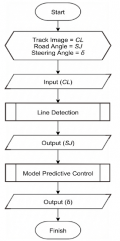
Explained in the system flowchart Figure 3, there is a declaration of variables to be used consisting of "Trajectory Image = CL", "Road Angle = SJ", and "Steering Angle = δ ". After the variable declaration, there is "INPUT (CL)", where the camera takes real-time recordings. The trajectory image that has been detected by the camera is immediately processed in "Line Detection", where this process will search for road boundaries and update the angle of change of the road. After the angle of change of the road is obtained, the angle of the road will be processed by "MPC" to predict how many degrees the steering angle will change so that the mobile robot does not leave the track. Then we get "OUTPUT (δ)" which will direct the robot to stay on its path, and the system is complete.
Figure 3. System flowchart
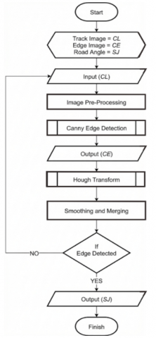
The system in digital image processing, where the camera detects the road and is processed in the line detection flowchart Figure 4. The system starts from the declaration of the variables "Edge Image = CE", and "Road Angle = SJ". Followed by "Image Pre-processing" where the image of the path will be improved image quality and remove noise in the image. After that the image will be processed in "Canny Edge Detection", where the road image will be taken only the edge of the road to determine the boundaries and shape of the path. After the edge of the road is known, it will be processed again using the "Hough Transform", in this process, the image will be drawn a straight line to determine the change in the angle of the road. After both are obtained, namely the edge boundary and the angle of the road, the results will be filtered and combined. To reduce the occurrence of unwanted detection, it is continued with conditioning, namely, whether the edge is detected. If the edge of the path is not detected, the system is restarted from "INPUT (CL)". And if the edge of the path is detected, then "OUTPUT (SJ)" is obtained, and the line detection process is complete.
Figure 4. Flowchart line detection
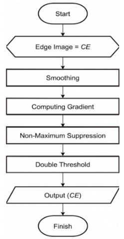
Figure 5 shows the flowchart of Canny edge detection, starting with the declaration of the variable “Citra Edge = CE”, followed by image smoothing using a Gaussian filter to reduce noise. Next, “Computing Gradient” is used to obtain the edge direction. After that, the non-maximum Suppression is performed to preserve edge peaks, followed by “Double Threshold” to identify strong and weak edges. Weak edges connected to strong edges are preserved. The result is a clear edge image, and the process is complete.
Figure 5. Flowchart edge detection
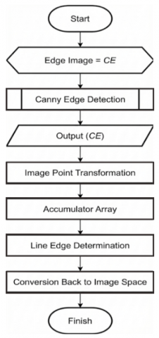
The Hough Transform is used to detect geometric shapes, such as straight lines, in the image of Figure 6. The process begins with the declaration of the variable “Citra Edge = CE” and continues with “INPUT (CE)”, then transforms the points in the image into a parameter space, where each line in the image is represented by two parameters: the line length (r) and the angle (θ), which describes the orientation of the line. Next, accumulation is carried out using an accumulator array to calculate the contribution of each point to these parameters, which are used to determine the existing lines. The lines with the highest contribution are considered as detected lines. The detected line information is then returned to the image space to be drawn, and the process is complete.
Figure 6. Hough Transform flowchart
Figure 7 shows the MPC flowchart, the system starts from the declaration of the variables “Road Angle = SJ”, and “Steering Angle = δ”, then there is “INPUT (SJ)” and calculates the objective function that measures how far the current system condition is from the desired reference condition. The objective function is then optimized to determine the optimal control, and then the “OUTPUT (δ)” is obtained, which will later be used by the servo motor as the Ackermann angle driver. Steering and the process are complete.

Figure 7. Flowchart Model Predictive Control (MPC)
2.6 Tool design
The mobile robot design in this study was made to resemble a four-wheeled vehicle in general, which uses an Ackermann steering mechanism. Steering. This design was chosen because it fits the characteristics of the robot, which will be designed to maneuver stably on curved paths. The robot's main structure uses acrylic, chosen for its sufficient strength to support all components.
The robot has four wheels, with the two front wheels serving as steering wheels and the two rear wheels serving as driving wheels. The Ackermann steering mechanism is controlled using a single servo motor connected to the two front wheels via a linkage system as shown in Figure 8. For forward movement, a single DC motor mounted on the axle is used. The gears transmit motor power to the rear wheels. This system allows the robot to perform turning maneuvers at angles adjusted automatically through MPC.

Figure 8. Robot component parts
The overall dimensions of the robot are 25 cm long, 15 cm wide, and 17 cm high, which are adjusted to be sufficient for testing in an indoor environment while still representing a small four-wheeled vehicle. The design of the mobile robot is shown in Figure 9.

Figure 9. Robot dimensions
Visually, the robot's view direction consists of a front view in Figure 10. You can see the camera facing forward and the servo drive, half of the body of which is under the car, and 2 LEDs located on the front of the robot to light the way if needed.

Figure 10. Front view
Rear view of Figure 11 shows 1 yellow button to set the robot's condition to be ready or not ready, and 1 red switch, which will be used as a switch. Supply from the battery.

Figure 11. Rear view
The side view in Figure 12 shows two wheels, namely the front wheel and the rear wheel, which are 15 cm apart. The camera orientation is slightly tilted downwards.

Figure 12. Side view
2.7 Road terrain
The terrain to be used is printed on . The road width is 20 cm. This has 2 colors, consisting of black as the main road area and white as the . This has several types of turns consisting of curved turns with an angle of 110° to 130°, T-turns with an angle of 90, and sharp turns with an angle of 30° to 50°. This design was created in as shown in Figure 13.

Figure 13. Road terrain
2.8 Electronic circuits
Electronic circuits on mobile, this robot is designed to connect all the main components so that the system can work properly. The ESP32 microcontroller acts as a control center that receives angle data from the computer via a WiFi network, then controls the robot's movement based on that data. The servo motor is connected to the ESP32 and is used to control the turning angle of the front wheels (Ackermann steering). A DC motor at the rear is used to move the robot forward. The DC motor is controlled through a motor driver, which is also connected to the ESP32. The electronic circuit is made using Fritzing software, as shown in Figure 14.

Figure 14. Electronic circuits
2.9 Ackermann steering kinematic model
The kinematic model of the robot in Figure 15 is used to predict the future position and orientation of the robot. The kinematic model of the robot is written in the form of equations of motion that depend on the speed and steering angle of the robot in Eq. (8).
$\operatorname{Tan}(\delta)=\frac{\mathrm{L}}{\mathrm{R}}$ (8)
Information:

Figure 15. Ackermann steering kinematic model [31-34]
3.1 Robot specifications
The selection of these components is based on the system requirements for running an autonomous robot, where the robot must be able to detect trajectories and perform precise turning maneuvers using the Ackermann steering mechanism. Furthermore, these specifications are adjusted to support the computation and actuator responses required by the MPC method. A brief list of the main components used in this robot can be seen in Table 1.
Table 1. Robot specifications
|
No. |
Component |
Type / Model |
Information |
|
1 |
Servo Motor |
Servo MG996R |
Steering Actuator |
|
2 |
DC motor |
JGA25 130 RPM |
Prime Mover |
|
3 |
Motorcycle Driver |
BTS7960 Module |
DC Motor Controller |
|
4 |
Encoder |
Magnetic |
Measuring wheel speed |
|
5 |
Camera |
Logitech C270 720p |
Image Input |
|
6 |
Microcontroller |
ESP32 DevKit V1 |
Control and Communication Unit |
|
7 |
Battery |
LiPo 3S 12V |
Key Resources |
3.2 Ackermann steering mechanic
The Ackermann steering mechanism on this robot is designed to ensure maneuver stability when the robot turns. This system is realized by using one servo motor Figure 16(a) as the main actuator that drives both front wheels through a mechanical linkage system (steering linkage) Figure 16(b).

(a)

(b)
Figure 16. (a) Bottom view of the Ackermann steering mechanism, (b) Top view of the Ackermann steering mechanism
3.3 Axle mechanic
The axle mechanism on this robot functions as the main power transmission system that converts the rotational energy from the DC motor into linear motion on the rear wheels (Figure 17). Based on the design that has been realized, this drive system uses a Rear Wheel Drive (RWD) configuration with one centralized drive motor.

Figure 17. Axle mechanism
3.4 Electronic circuits
The electronic circuit is the core of the robot control system in Figure 18, connecting the processing, sensors, and actuators. The entire robot's electrical system is centered on the ESP32 microcontroller, which is responsible for managing the flow of data and control signals.

Figure 18. Electronic circuits
3.5 Robot physics
The robot's physical structure is designed to resemble the structure of a conventional four-wheeled vehicle to accommodate the Ackermann steering mechanism. The robot's main structure is constructed using acrylic. This material was chosen based on its lightweight characteristics yet has sufficient strength to support all electronic components, batteries, and drive motors. Physically, the robot's body can be seen in Figure 19.

Figure 19. Robot physics
3.6 Servo motor calibration
Servo calibration was performed (Figure 20) to map the MPC steering output δ (deg) into a safe servo command range. The center position (straight motion) was identified, and the left/right mechanical limits were measured to avoid linkage saturation. These calibrated limits are used as the steering constraints (δ_min, δ_max) in the MPC implementation.

Figure 20. Servo motor calibration
3.7 Encoder sensor calibration
Encoder calibration was conducted to convert pulse counts into wheel speed v (m/s) in Figure 21. The pulses-per-revolution value was identified and combined with wheel diameter to obtain a speed conversion factor. The resulting speed estimate is used as a fixed parameter during the experiments.

Figure 21. Encoder sensor calibration
3.8 Camera calibration
In Figure 22, the camera tilt angle was adjusted to ensure a consistent ROI covering the lane ahead. This calibration improves the robustness of edge detection and the accuracy of θ_road and d_px estimation under varying lighting.

Figure 22. Camera calibration
3.9 Robot testing using the Model Predictive Control method
In Table 2, robot response data for several representative conditions during testing the MPC control system on the Ackermann steering robot. In general, the test results show that the MPC implementation is capable of producing stable steering behavior in various track conditions, including straight segments, moderate turns, sharp turns, and conditions with large lateral deviations.
Table 2. Robot response data
|
No |
Linta San's Condition |
Road Angle (°) |
X Deviation (px) |
MPC Angle (°) |
Smooth Angle (°) |
Servo |
|
1 |
Straight stable |
-1.49 |
15.29 |
0.00 |
-0.00 |
75 |
|
2 |
Medium left turn |
-21.08 |
0.00 |
-25.00 |
-24.47 |
99 |
|
3 |
Sharp left turn |
-32.10 |
100.08 |
-40.00 |
-39.32 |
114 |
|
4 |
Sharp right turn |
42.58 |
0.00 |
40.00 |
40.00 |
115 |
|
5 |
Right medium turn |
43.04 |
0.00 |
40.00 |
40.00 |
35 |
|
6 |
High light conditions |
±21–32 |
Varies |
On the road |
According to smoothing |
Varies |
In the straight road conditions of Figure 23, the road angle value is around 0° with slight variations due to image noise. The MPC responds by providing an MPC angle = 0° and a smooth angle = −0°, so that the robot maintains a stable direction of motion. A servo command value of around 75 indicates that the servo is in the center position according to calibration, indicating that the control has operated in a steady-state condition without oscillation.

Figure 23. Straight road
In the moderate turn in Figure 24, the road angle is detected at around ±20°–25°. The MPC produces an MPC angle close to this value, but slightly smoothed by the angle smooth filter. As a result, the robot enters the turn with a smooth transition without jerking movements. This indicates that the weighting in the MPC objective function is able to balance the need to follow the road angle and the limitations of steering dynamics.

Figure 24. Moderate curving road
In the sharp turn in Figure 25, the road angle reaches more than ±32° to ±43°, which is a critical condition for small robots with a limited turning radius. The MPC responds by generating a steering angle close to the maximum limit (±40°) but remains within the safe servo limits (35–115). Although there is a slight overshoot at the start of the maneuver, the smooth angle value dampens the sudden change so that the robot remains on track without going off track. This condition demonstrates the predictive ability of the MPC to anticipate changes in road angle several steps ahead.

Figure 25. Sharp turning road
The condition with a large lateral deviation (row 3, deviation 100px) shows that the robot is still able to correct itself back towards the centerline. This demonstrates the superiority of MPC in optimizing not only orientation but also lateral position errors simultaneously. The robot's success in returning to the center of the lane under this condition demonstrates the effectiveness of the two-state lane steering approach (yaw error + lateral deviation).
Furthermore, testing in a highly reflective area (row 6) demonstrates that the angular smoothing mechanism is able to prevent the servo response from following noisy line contour changes. This is important because uneven lighting is often a major challenge in vision-based systems.
Overall, the test results show that the integration of Canny–Hough-based line detection with the MPC algorithm results in adaptive, stable, and safe path tracking performance for the Ackermann steering mechanical system. The smooth steering response and the robot's ability to follow various types of turns indicate that the MPC parameter values used—including the prediction horizon, error penalty weighting, and control constraint limits—are in the optimal configuration for this trajectory scenario.
The test results show that the MPC algorithm is able to control the robot stably in various track conditions. On the straight segment, the measured road angle is only around −1.49° with a lateral deviation of 15.29 px, so that the MPC produces a steering command of 0.00° with a servo command of 75, which indicates the ideal steering position is at the center. On moderate turns, when the road angle reaches −21.08° and 43.04°, the MPC provides a correction of −25° to +40°, with a smooth angle at −24.47° and +40°, so that the robot is able to enter and exit turns without oscillation.
For sharp turns, the road angle increased to −32.10° and +42.58°, with a deviation even reaching 100.08 px in one scenario. In this critical condition, the MPC was still able to provide a maximum correction angle of ±40°, which was still within the safe servo operating limits (35–115). The servo command value reached 114–115 in the most extreme turns, but did not cause mechanical saturation or loss of control. The robot was still able to follow the path and return to the center of the track within several prediction cycles.
Furthermore, under high lighting conditions that produce reflections on the track surface, the road angle variation is in the range of ±21°–32°. MPC with smoothing is able to withstand sudden angular changes, maintaining the stability of the robot's motion so that steering commands do not follow image noise. Overall, MPC is proven to be able to maintain the robot's orientation and position simultaneously, follow the path with high precision, and produce smooth maneuvers in various degrees of turning and environmental conditions.
With stable performance at angles up to ±43° and deviations reaching 100px, it can be concluded that the MPC parameter configuration, servo constraint limits, and Canny–Hough-based line detection integration have worked optimally in producing a responsive and safe robot navigation system. These results confirm that MPC has great potential for application in service robots and indoor autonomous navigation systems that require precise maneuvers and adaptability to trajectory variations.
[1] Hartadi, F.T., Wicaksana, B.A., Saputro, H., Priambodo, A.S. (2024). Fuzzy control system for mobile robots: Case study of moving object tracking using webots simulation. Journal of Informatics and Applied Electrical Engineering, 12(3). https://doi.org/10.23960/jitet.v12i3.4608
[2] Syah, A., Caniago, D.P. (2023). Rancang Bangun Robot Mobile Pengawasan Berbasis IoT (Internet of Things) Menggunakan Kamera ESP-32. Jurnal Quancom: Quantum Computer Jurnal, 1(2): 16-20. https://journal.iteba.ac.id/index.php/jurnal_quancom/article/view/186.
[3] Dalimunthe, I.P., Nofryanti. (2020). The perspective of road users on online motorcycle taxis: The perspective on traffic jams. Economic Media, 20(1): 16-25. https://doi.org/10.30595/medek.v20i1.9513
[4] Yuzaeva, P.M., Wibisono, R.E. (2023). Geometric road planning design on bends using the Bina marga method and calculation of road user safety equipment requirements at Sta 11+800 to Sta 12+200 of the Bareng-Wonosalam Pasar Road section, Jombang Regency. Journal of Applied Transportation Publication Media, 1(1): 49-63.
[5] Wicaksono, D., Almeyda, D.P., Putra, I.M.M., Malihatuningrum, L. (2024). Analisis perbandingan metode pra pemrosesan citra untuk deteksi tepi Canny pada citra berbagai kondisi jalan menggunakan bahasa pemrograman Python. Jurnal Teknologi dan Ilmu Komputer Prima (JUTIKOMP), 7(1): 17-31. https://doi.org/10.34012/jutikomp.v7i1.3872
[6] Mwitta, C., Rains, G.C. (2024). The integration of GPS and visual navigation for autonomous navigation of an Ackerman steering mobile robot in cotton fields. Frontiers in Robotics and AI, 11: 1359887. https://doi.org/10.3389/frobt.2024.1359887
[7] Jian, Z.Z., Yan, Z.H., Lei, X.A., Lu, Z.H., Lan, B., Wang, X.Q., Liang, B. (2022). Dynamic control barrier function-based model predictive control to safety-critical obstacle-avoidance of mobile robot. arXiv preprint arXiv:2209.08539. https://doi.org/10.48550/arXiv.2209.08539
[8] Schwenzer, M., Ay, M., Bergs, T., Abel, D. (2021). Review on model predictive control: An engineering perspective. The International Journal of Advanced Manufacturing Technology, 117: 1327-1349. https://doi.org/10.1007/s00170-021-07682-3
[9] Liu, H., Shen, Y., Yu, S.J., Gao, Z.J., Wu, T. (2024). Deep reinforcement learning for mobile robot path planning. arXiv preprint arXiv:2404.06974. https://doi.org/10.48550/arXiv.2404.06974
[10] Divanny, S.R. (2024). Implementation of OpenCV and fuzzy logic controller for camera-based line follower in E-Puck robot simulation in Webots. Journal of Informatics and Applied Electrical Engineering, 12(3). https://doi.org/10.23960/jitet.v12i3.4718
[11] Ito, N., Okuda, H., Suzuki, T. (2023). Configuration-aware model predictive motion planning for Tractor–Trailer Mobile Robot. Advanced Robotics, 37(5): 329-343. https://doi.org/10.1080/01691864.2022.2126733
[12] Shih, C.H., Lin, C.J., Jhang, J.Y. (2023). Ackerman unmanned mobile vehicle based on heterogeneous sensors in navigation control applications. Sensors, 23(9): 4558. https://doi.org/10.3390/s23094558
[13] Rybczak, M., Popowniak, N., Lazarowska, A. (2024). A survey of machine learning approaches for mobile robot control. Robotics, 13(1): 12. https://doi.org/10.3390/robotics13010012
[14] Zhang, B., Okutsu, M., Ochiai, R., Tayama, M., Lim, H.O. (2023). Research on design and motion control of a considerate guide mobile robot for visually impaired people. IEEE Access, 11: 62820-62828. https://doi.org/10.1109/ACCESS.2023.3288152
[15] Tuleshov, A., Tuleshov, Y., Kuatova, M., Kamal, A., Kerimkulov, D. (2024). The synthesis of a two-circuit steering mechanism of the Ackerman transport mobile robot. Preprints.org. https://doi.org/10.20944/preprints202409.0709.v1
[16] Liu, L.Z., Chen, X.H., Zhu, S.Y., Tan, P. (2021). CondLaneNet: A top-to-down lane detection framework based on conditional convolution. In 2021 IEEE/CVF International Conference on Computer Vision (ICCV), Montreal, QC, Canada, pp. 3773-3782. https://doi.org/10.1109/ICCV48922.2021.00375
[17] Yoga, S.M.S., Pangaribuan, P., Fuadi, A.Z. (2022). Control of a wheeled robot as a self-driving car based on image processing with the fuzzy logic method. Journal of Computer Science and Informatics, 2(2): 77-92. https://doi.org/10.54082/jiki.25
[18] Ebel, H., Rosenfelder, M., Eberhard, P. (2024). Cooperative object transportation with differential-drive mobile robots: Control and experimentation. Robotics and Autonomous Systems, 173: 104612. https://doi.org/10.1016/j.robot.2023.104612
[19] Fuad, M., Wahyuni, S. (2022). Path planning and smoothing in maze exploration using virtual mobile robot-based modified probabilistic road map. In 2022 IEEE 8th Information Technology International Seminar (ITIS), Surabaya, Indonesia, pp. 15-20. https://doi.org/10.1109/ITIS57155.2022.10010054
[20] Ariska, M., Akhsan, H., Muslim, M. (2021). Modeling of Tippee Top (Tt) dynamics with non-holonomic constraints based on physics computation on a flat surface. Jurnal Pendidikan Fisika, 7(1): 20-25.
[21] Jumadi, J., Yupianti, Y., Sartika, D. (2021). Digital image processing for object identification using hierarchical agglomerative clustering methods. Journal of Science and Technology, 10(2): 148-156. https://doi.org/10.23887/jstundiksha.v10i2.33636
[22] Fadjeri, A., Saputra, B.A., Ariyanto, D.K.A., Kurniatin, L. (2022). Karakteristik morfologi tanaman selada menggunakan pengolahan citra digital. Jurnal Ilmiah Sinus (JIS), 20(2): 1-12. https://doi.org/10.30646/sinus.v20i2.601
[23] Guo, M.H., Xu, T.X., Liu, J.J., Liu, Z.N., Jiang, P.T., Mu, T.J. (2022). Attention mechanisms in computer vision: A survey. Computational Visual Media, 8(3): 331-368. https://doi.org/10.1007/s41095-022-0271-y
[24] Zhao, X., Wang, L.M., Zhang, Y.F., Han, X.M., Deveci, M., Parmar, M. (2024). A review of convolutional neural networks in computer vision. Artificial Intelligence Review, 57: 99. https://doi.org/10.1007/s10462-024-10721-6
[25] Zakaria, N.J., Shapiai, M.I., Ghani, R.A., Yassin, M.N.M., Ibrahim, M.Z., Wahid, N. (2023). Lane detection in autonomous vehicles: A systematic review. IEEE Access, 11: 3729-3765. https://doi.org/10.1109/ACCESS.2023.3234442
[26] Song, Y.P., Li, C.L., Xiao, S.Y., Zhou, Q.L., Xiao, H. (2024). A parallel Canny edge detection algorithm based on OpenCL acceleration. PLoS ONE, 19(1): e0292345. https://doi.org/10.1371/journal.pone.0292345
[27] Yang, L.J., Li, M.B., Wu, T.X., Bao, Y.F., Li, J.H., Jiang, Y. (2023). Geo-information mapping improves Canny edge detection method. IET Image Processing, 17(6): 1893-1904. https://doi.org/10.1049/ipr2.12764
[28] Zhao, K., Han, Q., Zhang, C.B., Xu, J., Cheng, M.M. (2021). Deep Hough transform for semantic line detection. IEEE Transactions on Pattern Analysis and Machine Intelligence, 44(9): 4793-4806. https://doi.org/10.1109/TPAMI.2021.3077129
[29] Andre, H., Sugara, B.A., Baharuddin, B., Fernandez, R., Pratama, R.W. (2021). Analisis komunikasi data jaringan nirkabel berdaya rendah menggunakan teknologi Long Range (LoRa) di daerah hijau Universitas Andalas. Jurnal Ecotipe, 9(1): 1-7. https://doi.org/10.33019/jurnalecotipe.v9i1.2480
[30] Wardani, A.K., Arifianto, A.S., Sirojudin, A., Aziza, A.N., Habibie, A.S. (2024). Implementation of digital twin with wireless data communication on liquid filling machine. JUKI: Journal of Computers and Informatics, 6(1): 46-54.
[31] Szott, S., Kosek-Szott, K., Gawłowicz, P., Gómez, J.T., Bellalta, B., Zubow, A. (2022). Wi-Fi meets ML: A survey on improving IEEE 802.11 performance with machine learning. IEEE Communications Surveys and Tutorials, 24(3): 1843-1893. https://doi.org/10.1109/COMST.2022.3179242
[32] Yulianto, Y. (2023). Relay driver based on Arduino UNO to bridge the gap of the digital output voltage of the node MCU ESP32. Engineering, Mathematics and Computer Science Journal (EMACS), 5(3): 129-135. https://doi.org/10.21512/emacsjournal.v5i3.9697
[33] Rombekila, A., Entamoing, B.L. (2022). IoT-based smart home prototype with Android mobile phone using NodeMCU ESP32. AMATA Engineering Journal, 3(1): 32-37. https://doi.org/10.55334/jtam.v3i1.275
[34] Raouf, I., Kumar, P., Kim, H.S. (2024). Deep learning-based fault diagnosis of servo motor bearings using the attention-guided feature aggregation network. Expert Systems with Applications, 258: 125137. https://doi.org/10.1016/j.eswa.2024.125137