Huu-Khanh Doan*![]() | Trung-Phuc Mac
| Trung-Phuc Mac![]() | Anh-Tuan Dinh
| Anh-Tuan Dinh![]() | Hoang-Binh Trong Nguyen
| Hoang-Binh Trong Nguyen![]()
© 2026 The authors. This article is published by IIETA and is licensed under the CC BY 4.0 license (http://creativecommons.org/licenses/by/4.0/).
OPEN ACCESS
Data-driven predictive maintenance for marine diesel engines is hindered by the scarcity of failure data and safety risks of onboard validation. Addressing this, we propose an integrated Hardware-in-the-Loop (HIL) framework for safe diagnostic algorithm development. Unlike software-only simulations, this approach utilizes a Siemens S7-1200 PLC and Delta HMI to mimic thermodynamic sensor outputs of a Daihatsu 6PSHTb-26D engine based on physics-based models. To demonstrate Operational Technology and Information Technology (OT-IT) convergence, a centralized architecture uses Kepware middleware to synchronize industrial control data with a SQL Server database. As a proof-of-concept, a hybrid diagnostic algorithm combining Receiver Operating Characteristic (ROC)-optimized adaptive thresholds and Multi-Layer Perceptron (MLP) networks was deployed. Validation confirms a high emulation fidelity (3.24% error), while the Artificial Neural Networks (ANNs) achieves superior accuracy (RMSE 0.0737℃) and real-time speed (0.041 ms). This validates PLC-based signal emulation as a cost-effective testbed for maritime AI applications before shipboard deployment.
marine diesel engine, Hardware-in-the-Loop, Operational Technology and Information Technology, convergence, PLC-based signal emulation, hybrid ANN
1.1 Background and motivation
Marine diesel engines, such as the Daihatsu 6PSHTb-26D, serve as the prime movers for a vast majority of merchant vessels. Ensuring their reliability is paramount for maritime safety and economic efficiency. Conventionally, maintenance strategies have relied on scheduled preventive maintenance. However, with the advent of Industry 4.0, there is a paradigm shift towards Condition-Based Maintenance (CBM). Recent systematic reviews indicate that data-driven approaches, particularly Deep Learning (DL), are becoming the dominant trend in maritime predictive maintenance [1]. Algorithms such as Convolutional Neural Networks (CNNs) and Temporal Convolutional Networks (TCNs) have demonstrated superior performance in feature extraction compared to traditional methods [2].
1.2 The challenge: Data scarcity and validation paradox
Despite the theoretical potential of AI, its deployment in the actual maritime sector faces a critical bottleneck: the lack of a verifiable testing environment. Advanced models require not only massive amounts of data for training but also ground-truth scenarios for validation. Currently, three specific limitations hinder the transition of research algorithms to shipboard application:
1.3 Related works and research gap
To address data limitations, researchers have explored several approaches. Transfer Learning has been utilized to adapt knowledge from related domains [3, 4], but this still relies on the existence of a high-quality source dataset. Others employ thermodynamic software (e.g., AVL Boost, GT-Power) or Digital Twins to generate synthetic data [5, 6]. While effective for generating data, these purely software-based simulations often lack the Hardware-in-the-Loop (HIL) connectivity required to validate the end-to-end data pipeline. There is a notable gap in the literature regarding low-cost, physical testbeds that allow researchers to validate not just the algorithm, but the entire monitoring architecture—from sensor signal generation to database logging and SCADA visualization—before deploying on a real ship.
While commercial HIL platforms such as dSPACE or OPAL-RT have been successfully employed in marine research for high-speed combustion control and fuel injection analysis [7], they are often prohibitively expensive and rely on proprietary hardware that differs significantly from actual shipboard automation. These systems operate at microsecond-level cycle times, which is essential for crank-angle resolved simulations but excessive for general condition monitoring. In contrast, this study proposes a cost-effective framework using the industrial Siemens S7-1200 PLC. Although its millisecond-level scan time is slower, it is sufficient for emulating thermodynamic process parameters (e.g., temperatures, pressures) characterized by high thermal inertia. The primary distinction is our focus on the "Operational Technology and Information Technology (OT-IT) validation" of the diagnostic pipeline rather than combustion physics. A detailed quantitative comparison between the proposed PLC-based approach and commercial HIL solutions is presented in Table 1.
Table 1. Quantitative comparison between commercial HIL and proposed PLC-based emulation
|
Feature |
Commercial HIL (e.g., dSPACE, OPAL-RT) |
Proposed PLC-Based Emulation (Siemens S7-1200) |
Comparative Advantage of Proposal |
|
Cost |
High ($10,000 - $50,000+) |
Low (< $500) |
> 20x Cost Reduction, accessible for mass deployment. |
|
Cycle Time |
μs-level (Microsecond) |
ms-level (5-10 ms) |
Sufficient for process parameters (Temp, Pressure) which have high thermal inertia. |
|
Connectivity |
Proprietary / Lab protocols |
Standard Industrial Protocols (S7 Comm, OPC UA, Modbus) |
Native integration with shipboard SCADA without converters. |
|
Target User |
R&D Engineers / Scientists |
Automation Engineers / Crew |
Aligned with actual workforce skills. |
|
Focus |
Combustion physics, High-speed control |
OT-IT Integration, Diagnostic logic |
Validates the System Architecture under realistic comms constraints. |
1.4 Contribution of this paper
Addressing these gaps, this study proposes a HIL Framework using a PLC-based Signal Emulation Strategy. Unlike static datasets or purely virtual models, our approach provides a physical interface to validate the real-time diagnostic pipeline. Specifically, this study offers three key contributions:
1.5 Organization of the paper
The remainder of this paper is organized as follows: Section 2 presents the overall system architecture, detailing the closed-loop data flow between the physical emulation layer and the intelligent processing core via SQL Server integration. Section 3 elaborates on the methodology, including the hardware setup of the simplified simulation kit, the mathematical modeling for signal generation, and the implementation of the hybrid diagnostic algorithm. Section 4 provides a comprehensive analysis of the experimental results, covering the HIL framework fidelity validation, the determination of adaptive thresholds using ROC analysis, and the real-time performance evaluation on the Edge device. Finally, Section 5 concludes the paper and outlines future research directions for commercial SCADA deployment.
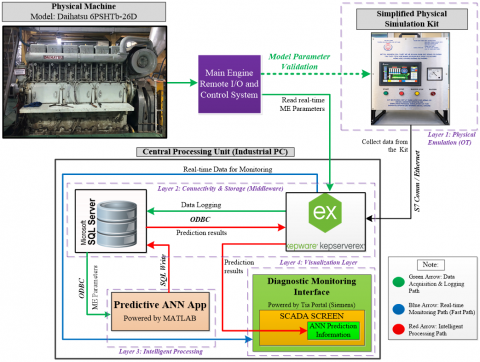
To validate the proposed hybrid diagnostic algorithm, a comprehensive HIL architecture was designed to facilitate the convergence of OT and IT. As illustrated in Figure 1, the system operates on a centralized data exchange model, structured into two primary functional blocks.
2.1 Physical emulation and connectivity (Layers 1&2)
The foundation of the framework is the Physical Emulation Layer, which functions as the OT source. Instead of relying on static datasets, this layer executes real-time thermodynamic models to mimic the transient behaviors of a Daihatsu 6PSHTb-26D engine. Crucially, it features a Fault Injection Interface, enabling the deterministic generation of labeled failure data for algorithm validation. To bridge the OT-IT gap, the Connectivity Layer acts as a middleware gateway. It communicates with the PLC via the S7 Ethernet protocol at a high-speed polling cycle of 100 ms for real-time monitoring. Meanwhile, to optimize storage efficiency for the diagnostic algorithm, the ODBC Data Logger is configured to buffer this data into the SQL Server database at a 1-second sampling rate. To ensure data consistency between the writing and reading processes, the transaction isolation level is set to 'Read Committed'.
2.2 Intelligent processing and visualization (Layers 3&4)
The computational core is the Intelligent Processing Layer, hosted on an Edge Industrial PC. A custom-built diagnostic service asynchronously queries the latest buffered data from the SQL Server and executes the Hybrid ANN Algorithm. This decoupled design allows the MATLAB-based engine to process complex logic without requiring fragile, direct connections to the control hardware. Finally, the diagnostic results are encapsulated and written back to the database to be retrieved by the Visualization Layer. This interface decodes the status to provide real-time situational awareness for operators, completing the closed-loop information flow.
Figure 1. Functional architecture of the proposed HIL framework
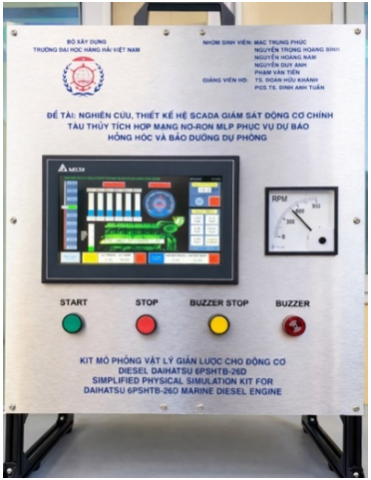
3.1 Development of the Simplified Physical Simulation Kit
To mitigate operational safety risks, a Simplified Physical Simulation Kit was developed as a HIL testbed (Figure 2(a)). Centered around a Siemens S7-1200 CPU 1215C PLC and a 10-inch Delta HMI, the system employs a Signal Emulation Strategy rather than static physical sensors. The PLC executes thermodynamic algorithms to generate real-time virtual signals (e.g., 4-20 mA, 0-10 V) for visualization. Crucially, the HMI serves as a Synthetic Fault Injection interface, enabling the generation of labeled data by modifying internal coefficients such as friction $\left(K_{ {fric }}\right)$ or cooling efficiency $\left(\eta_{ {cool }}\right)$.
(a)
(b)
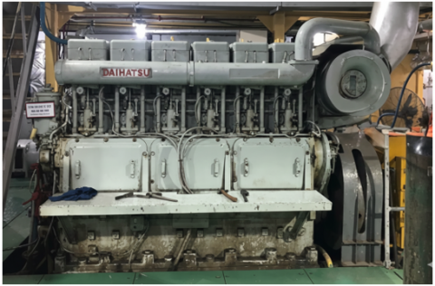
Figure 2. The experimental setup: (a) The fabricated Simplified Physical Simulation Kit powered by Siemens S7-1200 PLC and Delta HMI; (b) The actual Daihatsu 6PSHTb-26D marine diesel engine used as the reference model
3.2 Mathematical modeling and diagnostic metrics
To validate the proposed diagnostic framework within a realistic automation environment, a HIL strategy was employed. Aligning with recent SCADA architectures utilizing Siemens S7-1200 controllers [8], physics-based mathematical models were embedded directly into the PLC memory.
While vibration and acoustic analysis offer high sensitivity for fault detection, retrofitting such sensors on existing fleets faces significant cost and bandwidth barriers. To ensure cost-effectiveness and alignment with the standard instrumentation of the reference Daihatsu 6PSHTb-26D engine (Figure 2(b)), this study focuses exclusively on thermodynamic and process parameters. Consequently, the emulation logic addresses five representative Diagnostic Indicators (DIs), derived from fundamental thermodynamics [9-12] and fluid mechanics [13].
3.2.1 Exhaust Gas Temperature (EGT) modeling (DI1)
The EGT dynamics are simulated in three stages: steady-state estimation, fault injection, and thermal inertia. First, the base thermodynamic temperature $\left(T_{{Base }}\right)$ is computed.
While basic control models often simplify the EGT-Load relationship as linear, established literature on control-oriented engine modeling [12] indicates that the thermal response is inherently non-linear due to the variable efficiency of the turbocharger and changing air-fuel ratios. To capture this curvature within the PLC's real-time constraints (without using computationally heavy Wiebe functions), we apply a second-order polynomial correction:
$T_{{Base }}=T_{{Coolant }}+\left(K_{R P M} \cdot n\right)+\left(K_{ {Load } 1} \cdot L \cdot n\right)+\left(K_{{Load } 2} \cdot L^2 \cdot n\right)$ (1)
where, $T_{{Coolant }}$ is the ambient coolant temperature (℃), n is the engine speed (rpm), and L is the dimensionless load factor $(0 \div 1), K_{R P M}, K_{ {Load } 1}$ and $K_{ {Load } 2}$ are empirical coefficients representing speed-dependent friction, linear combustion heat release, and non-linear efficiency corrections, respectively.
To simulate cylinder-specific faults (DI1), a deviation offset is applied to a specific cylinder i based on a fault intensity input $F_{E G T, i}(0 \div 1)$:
$T_{ {Target }, i}=T_{ {Base }} \cdot\left(1+K_{{Fault }} \cdot F_{E G T, i}\right)$ (2)
where, $K_{{Fault}}$ is the sensitivity coefficient. Finally, to mimic the response time of industrial thermocouples [14], a discrete first-order lag filter is applied:
$T_{E G T, i}(k)=T_{E G T, i}(k-1)+\left[T_{T a r g e t, i}-T_{E G T, i}(k-1)\right] \cdot \frac{\Delta t}{\tau}$ (3)
Here, $\Delta t$ is the PLC scan cycle time (s) and $\tau$ is the sensor thermal time constant (s).
3.2.2 Lube Oil Pressure and viscosity dynamics (DI2)
The lubrication system is modeled as a coupled thermal-hydraulic system consistent with marine machinery principles [15, 16]. First, similar to the cooling system, the Lube Oil Temperature ($T_{L O}$) dynamics are simulated based on the heat balance between friction generation and oil cooling efficiency. The instantaneous temperature is updated via a lag filter:
$T_{L O}(k)=T_{L O}(k-1)+\left[T_{ {Target }, L O}-T_{L O}(k-1)\right] \cdot \frac{\Delta t}{\tau_{L O}}$ (4)
where, $T_{{Target,LO }}$ is the steady-state target temperature (℃), $\Delta t$ is the scan cycle time (s), and $\tau_{L O}$ is the thermal time constant of the oil sump (s).
Crucially, the oil viscosity ($\mu$) is dynamically updated based on this real-time temperature using the Andrade Equation [17, 18]:
$\mu=A \cdot e^{\frac{B}{T_{L O}+273.15}}$ (5)
where, A and B are empirical constants specific to the SAE-40 oil grade.
The pressure generation logic incorporates both the electric priming pump and the engine-driven mechanical pump. The mechanical pressure ($P_{ {Mech }}$) is calculated as:
$P_{ {Mech }}=\left(K_{ {Pump }} \cdot n\right) \cdot\left(1+K_{{Visc }} \cdot\left(\mu-\mu_{ {Ref }}\right)\right)$ (6)
where, n is engine speed (rpm), $K_{ {Pump }}$ is the pump efficiency factor (bar/rpm), $K_{V i s c}$ is the viscosity correction coefficient, and $\mu_{ {Ref }}$ is the reference viscosity at normal operating temperature.
To validate the diagnostic algorithms, the final source pressure is determined by a "Check Valve" logic (max) and then degraded by Filter Clogging ($F_{ {Clog }}$) and Bearing Wear ($F_{ {Wear }}$) faults:
$P_{{Source }}=\max \left(P_{ {Elec }}, P_{ {Mech }}\right)$ (7)
$P_{L O}=\min \left(P_{ {Set }}, P_{ {Source }} \cdot\left(1-K_F \cdot F_{ {Clog }}\right) \cdot\left(1-K_W \cdot F_{ {Wear }}\right)\right)$ (8)
where, $P_{{Elec }}$ is the priming pump pressure (bar), $P_{{Set }}$ is the relief valve limit (bar), and $K_F, K_W$ are the dimensionless fault severity scaling factors.
3.2.3 Cooling system thermal equilibrium (DI3)
The Jacket Water (JW) temperature model balances heat generation ($Q_{J W}$) against cooling efficiency [10]. The heat rejection is estimated to be proportional to speed and load:
$Q_{J W}=\left(K_{J W, n} \cdot n\right)+\left(K_{J W, L} \cdot L \cdot n\right)$ (9)
where, $K_{J W, n}$ and $K_{J W, L}$ are heat transfer coefficients. The target equilibrium temperature is derived by applying a cooling efficiency factor $\eta_{ {Cooling }}$:
$T_{{Target }}=T_{ {Amb }}+\frac{Q_{J W}}{\eta_{ {Cooling }}}$ (10)
Under fault conditions (DI3 - Radiator Fouling), $\eta_{{Cooling }}$ is reduced from 1.0 via the HMI. Finally, to simulate the significant thermal inertia of the coolant volume, the real-time temperature is updated via a first-order lag function:
$T_{J W}(k)=T_{J W}(k-1)+\left[T_{ {Target }}-T_{J W}(k-1)\right] \cdot \frac{\Delta t}{\tau_{J W}}$ (11)
where, $\tau_{J W}$ is the thermal time constant of the cooling system.
3.2.4 Governor dynamics and stability (DI4)
The engine speed control is governed by a Finite State Machine (FSM). To simulate the mechanical moment of inertia, the speed transition follows a ramp function with a saturation limiter (sat):
$n_{{Ramp }}(k)=n(k-1)+\operatorname{sat}\left(\frac{n_{{Target }}-n(k-1)}{\Delta t}, K_{ {Ramp }}\right) \cdot \Delta t$ (12)
where, $K_{R a m p}$ is the maximum acceleration rate (${rpm} / {s}^2$).
Furthermore, acknowledging the importance of stability analysis in control systems [19], a deterministic noise signal is injected to validate the detection algorithm. Although actual governor instability typically manifests as a non-linear limit cycle, this study deliberately employs a fixed-frequency sinusoidal waveform as a standardized Fault Injection signal. This approach isolates the frequency-based instability from stochastic mechanical friction, allowing for the precise calibration of the Neural Network’s frequency extraction sensitivity. The injected speed is defined as:
$n_{{Final }}=n_{{Ramp }}(k)+\left(K_{{Noise }} \cdot F_{ {Gov }}\right) \cdot \sin (\omega t)$ (13)
where, $F_{G o v} F_{G o v}$ is the fault intensity, $K_{N o i s e}$ is the maximum noise amplitude and $\omega$ is the oscillation frequency $({rad} / {s})$.
3.2.5 Starting air pneumatic decay (DI5)
The starting air pressure ($P_{A i r}$) is modeled using a differential mass balance equation [13]. The net rate of pressure change combines charging ($R_{C h g}$), consumption ($R_{ {Cons }} R_{ {Cons }}$), and leakage ($R_{ {Leak }}$):
$R_{ {Leak }}=-K_{{Leak }} \cdot F_{ {AirLeak }}$ (14)
$\frac{d P_{A i r}}{d t}=R_{C h g}+R_{C o n s}+R_{ {Leak }}$ (15)
where, $K_{ {Leak }}$ is the leakage coefficient and $F_{ {AirLeak }}$ is the fault variable $(0 \div 1)$.
Since the PLC operates in discrete time, it explicitly integrates this rate of change to update the system pressure in real-time:
$P_{A i r}(k)=P_{A i r}(k-1)+\frac{d P_{A i r}}{d t} \cdot \Delta t$ (16)
where, $P_{ {Air }}(k)$ is the instantaneous air pressure (bar). This formulation allows the "Air Leakage" logic (DI5) to be validated against mathematically defined decay rates.
3.3 The hybrid diagnostic algorithm
To ensure the proposed solution remains cost-effective and faithful to the configuration of the reference Daihatsu 6PSHTb-26D engine, this study restricts its scope to thermodynamic and process parameters. Consequently, five representative Dis were selected. These DIs are processed by a hybrid algorithm running on MATLAB, categorized into two groups: Rule-based Statistical Logic and Multi-Layer Perceptrons (MLP)-based Normality Modeling.
3.3.1 Group 1: Rule-based statistical logic
Parameters with linear characteristics or distinct physical thresholds are monitored using statistical rules.
DI1 (EGT Deviation): This indicator quantifies the thermal unevenness of combustion. It is calculated as the maximum deviation of any single cylinder's temperature from the instantaneous average of all six cylinders:
$T_{a v g}=\frac{1}{6} \sum_{i=1}^6 T_{E G T, i}$ (17)
$D I 1=\max _{i=1 \ldots 6}\left(\left|T_{E G T, i}-T_{ {avg }}\right|\right)$ (18)
DI4 (Governor Stability): This metric assesses the mechanical stability of the speed control loop. It is defined as the Oscillation Amplitude ($A_{g o v}$) of the engine speed within a sliding time window (W), active only when the engine is in the running state (SE = 2):
$D I 4=\max _{t \in W}(n)-\min _{t \in W}(n)$ (19)
DI5 (Air Leak Rate): This indicator detects pneumatic leakage severity by monitoring the instantaneous rate of pressure change. It is formally defined as the time derivative of the air pressure, approximated in the discrete domain as:
$D I 5=\frac{d P_{A I R}}{d t} \approx \frac{P_{A I R}(t)-P_{A I R}(t-\Delta t)}{\Delta t}$ (20)
3.3.2 Group 2: Multi-Layer Perceptrons-based normality modeling
Complex non-linear parameters are modeled using MLP based on standard pattern recognition theory. Adopting a Normality Modeling approach, the networks were trained exclusively on 11,520 samples of healthy data to learn the ideal engine behavior across the full operating range.
To ensure the reproducibility of the experimental results, the specific architecture and training hyperparameters are detailed in Table 2. The model uses a deep topology optimized for non-linear regression using the Levenberg-Marquardt algorithm.
Faults are detected by analyzing the Residual (R) between the measured real-time value and the MLP prediction. The residuals for the two non-linear indicators are defined using the general functional form as follows:
DI2 (Lube Oil Residual): The network predicts the expected oil pressure based on the current engine speed, oil temperature, and load factor. The residual reflects anomalies such as pump degradation or filter clogging:
$D I 2=P_{L O}-P_{ {pred }}\left(n, T_{L O}, L\right)$ (21)
DI3 (Jacket Water Residual): Similarly, the expected cooling water temperature is predicted to detect cooling efficiency losses (e.g., radiator fouling):
$D I 3=T_{J W}-T_{{pred }}\left(n, T_{L O}, L\right)$ (22)
Table 2. Configuration of the proposed Multi-Layer Perceptrons (MLP) network
|
Parameter |
Value/Setting |
|
Topology |
[3 - 50 - 90 - 1] |
|
Algorithm |
Levenberg-Marquardt (trainlm) |
|
Activation Fcn. |
Tansig (Hidden) / Purelin (Output) |
|
Perf. Metric |
Mean Squared Error (MSE) |
|
Target Goal |
5 |
|
Learning Rate |
1 |
|
Max Epochs |
5000 |
The selection of this specific topology [3-50-90-1] was based on a preliminary empirical grid search, which identified it as the optimal configuration balancing learning capability (RMSE) and computational efficiency (inference time) for the target IPC hardware.
3.3.3 Output Bit-Packing
To optimize storage and transmission bandwidth, the diagnostic status of all five DIs (classified into Normal, Warning, or Alarm levels) is encoded into a single 16-bit integer (Packed_Alarm_Integer) before being written to the SQL Server.
4.1 HIL framework validation and data generation strategy
4.1.1 Data acquisition protocol and dataset partitioning
To develop a robust diagnostic model, a comprehensive dataset covering various operational regimes was first acquired using the proposed HIL framework. The data collection strategy was explicitly designed to serve two distinct purposes: (1) training the normality model using healthy data under varying loads, and (2) calibrating the diagnostic thresholds using synthetic fault data.
The detailed experimental specifications are summarized in Table 3. To systematically capture these datasets, the experimental procedure was executed in two sequential phases:
Table 4 presents a snapshot of the logged data, illustrating the contrast between the healthy baseline (Phase 1) and the critical anomalies captured during the fault injection scenarios (Phase 2).
Table 3. Experimental scenarios for data acquisition
|
Fault Label |
Condition |
Severity Levels (%) |
Speed Levels |
Load (%) |
Sampling Duration |
|
0 |
Normal Operation |
0% |
1, 3, 5, 7 |
0%, 25%, 50%, 80% |
15 min / level |
|
1 |
DI1 Fault (EGT Deviation) |
15, 25, 50, 80% |
1, 3, 5, 7 |
0%, 25%, 50%, 80% |
1.5 min / level |
|
2 |
DI2 Fault (P_LO Drop) |
15, 25, 50, 80% |
1, 3, 5, 7 |
50% |
1.5 min / level |
|
3 |
DI3 Fault (T_JW Overheat) |
15, 25, 50, 80% |
1, 3, 5, 7 |
0%, 25%, 50%, 80% |
1.5 min / level |
|
4 |
DI4 Fault (Gov. Hunting) |
15, 25, 50, 80% |
1, 3, 5, 7 |
50% |
1.5 min / level |
|
5 |
DI5 Fault (Air Leakage) |
15, 25, 50, 80% |
1, 3, 5, 7 |
50% |
1.5 min / level |
Table 4. Snapshot of the logged dataset illustrating both Normal (Phase 1) and Fault (Phase 2) conditions
|
LogID |
Time |
n_Actual |
n_Target |
Load (%) |
P_LO |
T_LO |
T_JW |
P_air |
EGT_1 |
… |
EGT_6 |
Status |
|
119 |
33:33.8 |
249.99 |
250 |
25% |
3.28 |
38.26 |
41.04 |
17.00 |
103.94 |
… |
104.47 |
Normal |
|
8180 |
54:52.2 |
406.66 |
406.66 |
0% |
3.5 |
39.32 |
43.46 |
17.00 |
150.47 |
… |
151.23 |
Fault 2 |
|
10035 |
38:03.1 |
563.31 |
563.33 |
50% |
3.5 |
42.92 |
51.45 |
17.50 |
197.01 |
… |
198.00 |
Fault 3 |
|
11619 |
20:57.5 |
719.54 |
720 |
80% |
3.5 |
58.82 |
62.70 |
17.50 |
243.57 |
… |
244.80 |
Fault 4 |
4.1.2 Multi-source Model Validation
To rigorously verify the fidelity of the proposed polynomial emulation model, a comparative analysis was conducted across a comprehensive set of 4 distinct operating points, covering the engine's functional range.
Data Source Construction: Given the specific constraints of the laboratory facility, which is currently configured for no-load testing, a synchronized validation strategy was established to ensure consistency:
Quantitative Verification: The model's accuracy was quantified using the Root Mean Square Error (RMSE) metric. To ensuring a rigorous assessment, the RMSE calculation was restricted to the thermodynamic state variables (EGT and $T_{J W}$) across the measured experimental dataset (Points P1-P3). The Lube Oil Pressure ($P_{L O}$) was excluded from the error metric as it functions as a controlled variable saturated at the safety valve setpoint.
$R M S E_{\%}=\frac{1}{N} \sum_{i=1}^N\left|\frac{y_{ {sim}, i}-y_{{ref}, i}}{y_{ {ref }, i}}\right| \times 100 \%$ (23)
As detailed in Table 5, the analysis yields a global average deviation of approximately 3.24%. This marginal discrepancy is attributed to the conservative heat transfer coefficients used in the model, which slightly underestimate the convective heat loss to the ambient environment compared to the actual laboratory conditions. Since the error remains well below the generally accepted tolerance for engineering emulation models (< 5%), the proposed Digital Twin is confirmed to have high fidelity.
Table 5. Validation of simulation model against measured and standard reference data
|
Operating Point |
Data Source |
Speed (rpm) |
EGT (℃) |
PLO (Bar) |
TJW (℃) |
|
P1 (No Load) |
Ref. (Measured) |
249.9 |
101.6 |
3.50 |
41.5 |
|
Sim. (Model) |
250.0 |
104.9 |
3.50 |
42.8 |
|
|
P2 (No Load) |
Ref. (Measured) |
484.9 |
170.1 |
3.50 |
53.2 |
|
Sim. (Model) |
485.1 |
175.5 |
3.50 |
54.9 |
|
|
P3 (No Load) |
Ref. (Measured) |
641.6 |
215.8 |
3.50 |
61.0 |
|
Sim. (Model) |
641.7 |
222.5 |
3.50 |
62.9 |
|
|
P4 (Rated Load) |
Ref. (Manual) |
720.0 |
< 450 [20] |
3.50* |
< 80 [20] |
|
Sim. (Model) |
720.0 |
418.9 |
3.50 |
77.6 |
Note:
4.2 Algorithmic performance and robustness analysis
4.2.1 Comparative assessment with baseline algorithms
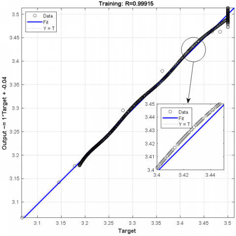
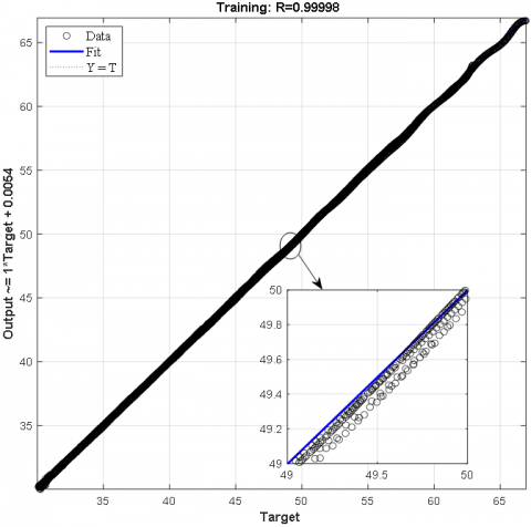
Evaluation of Normality Models: Before establishing the diagnostic thresholds, the predictive accuracy of the Normality Models was rigorously evaluated using the healthy dataset (Label 0). The regression analysis for the non-linear indicators—Lube Oil Pressure (DI2) and Jacket Water Temperature (DI3)—is presented in Figure 3. The evaluation focuses on three key performance aspects:
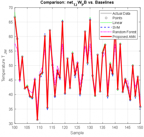
Comparative Benchmarking: Following the internal validation, a comparative analysis was conducted to benchmark the proposed ANN against standard algorithms. The quantitative performance metrics are summarized in Table 6. Additionally, Figure 4 provides a visual comparison of the tracking performance using a representative window of 150 testing samples for the target variable Jacket Water Temperature ($T_{J W}$).
Quantitatively, the proposed ANN ([3-50-90-1] topology) demonstrated superior accuracy, achieving a minimal RMSE of 0.0737℃ and an R2 of 0.9999. In contrast, linear models (LR, SVM) plateaued at an RMSE of ≈ 0.64℃, while the Random Forest algorithm yielded the highest error (2.82℃) due to its limitation in modeling continuous thermodynamic gradients.
Regarding implementation, the ANN’s inference time of 0.0410 ms is fully compatible with the proposed HIL architecture. Although marginally higher than simple linear algorithms, this latency is negligible compared to the standard PLC-to-IPC communication cycle (100 ÷ 200 ms). Consequently, the model ensures instantaneous processing on the Edge IPC without inducing data backlogs, satisfying the strict requirements for real-time monitoring.
Table 6. Performance benchmarking of diagnostic algorithms
|
Algorithm |
RMSE (℃) |
MAE (℃) |
R2 Score |
Inference Time (ms) |
|
Proposed ANN |
0.0737 |
0.0582 |
0.9999 |
0.0410 |
|
Linear Regression (LR) |
0.6437 |
0.5215 |
0.9645 |
~ 0.0001 |
|
Support Vector Machine (SVM) |
0.6431 |
0.5190 |
0.9650 |
0.0047 |
|
Random Forest (RF) |
2.8236 |
2.1450 |
0.8842 |
0.0151 |
(a)
(b)
Figure 3. Regression analysis of the MLP Normality Models: (a) Predicted vs. Target Lube Oil Pressure (R = 0.99915); (b) Predicted vs. Target Jacket Water Temperature (R = 0.99998)
Figure 4. Performance comparison with standard algorithms
4.2.2 Dynamic response and load sensitivity analysis
While the low RMSE values established in Section 4.2.1 confirm the model's static accuracy, a robust diagnostic system must also distinguish between actual faults and natural "transient errors" caused by thermal lag during maneuvering. Therefore, this section evaluates the ANN's dynamic robustness under extreme load changes and its sensitivity across the full operational range.
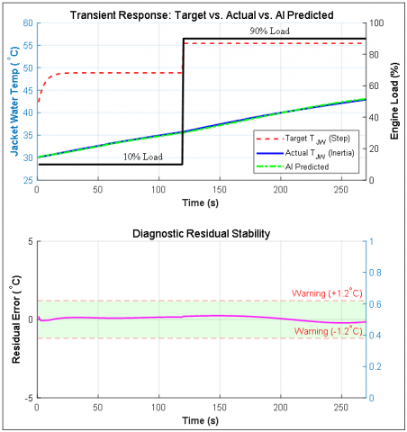
Transient Response and False Alarm Rejection: To verify the system’s immunity to false alarms, a rigorous step-response test was executed by abruptly increasing the engine load from 10% to 90% (a severe load step scenario). Figure 5 visualizes the system's performance during this transient phase. As observed, while the Load command (black line) exhibits an instantaneous step change, the actual Jacket Water temperature (blue line) rises gradually due to the physical thermal mass of the engine. Crucially, the ANN predicted value (green line) accurately tracks this gradual physical trajectory rather than overfitting to the abrupt load input. This capability is attributed to the network effectively utilizing the Lube Oil Temperature ($T_{L O}$) as an inertia-aware feature. Consequently, the diagnostic residual remains remarkably stable, consistently staying below 1.0℃—well within the defined safety threshold of $\pm 1.2^{\circ} \mathrm{C}$. This confirms that the system yields zero false-positive rates during dynamic maneuvering.
Figure 5. Transient response validation under extreme load stepping (10% ÷ 90%)
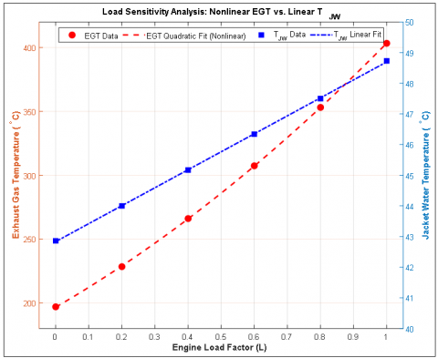
Load Sensitivity and Physical Generalizability: To further demonstrate the framework's generalizability, a comprehensive load sensitivity experiment was conducted by varying the engine load factor (L) from 10% to 100%. Figure 6 illustrates that the ANN successfully learned the distinct physical behaviors of different subsystems:
These results confirm that the proposed ANN architecture successfully learns both the fast-dynamic non-linear characteristics of the combustion process and the high-inertia stable dynamics of the cooling system, ensuring robust fault detection across all operational regimes.
Figure 6. Load sensitivity (10% ÷ 100%)
4.3 Determination of adaptive thresholds
To address the limitations of fixed-value thresholds and satisfy the requirement for a robust monitoring scheme, this study proposes a statistical Adaptive Threshold Mechanism. Unlike static limits, these thresholds dynamically account for the inherent stochastic noise of the engine and hardware uncertainties.
4.3.1 Mathematical formulation
The fault detection boundaries are formulated based on the principles of Statistical Process Control (SPC) [21]. Specifically, to accommodate both the stochastic nature of the engine process and hardware limitations, the adaptive threshold ($T_{t h}$) is defined as:
$T_{t h}=\left|\mu_{ {res }}\right|+k \cdot \sigma_{ {res }}+\epsilon_{{sensor }}$ (24)
where, $\mu_{ {res }}$ is the mean bias of the prediction residual (systematic error); $\sigma_{ {res }}$ is the standard deviation of the residual (noise floor); k is the sensitivity coefficient optimized via ROC analysis (determining how many standard deviations constitute an anomaly) and $\epsilon_{{sensor }}$ is the instrumentation uncertainty margin.
Crucially, this mechanism allows for periodic recalibration. As the engine ages and mechanical clearances increase (leading to higher baseline noise $\sigma_{ {res }}$, the thresholds can be automatically updated by recalculating standard deviation, thereby preventing false alarms throughout the engine's lifecycle.
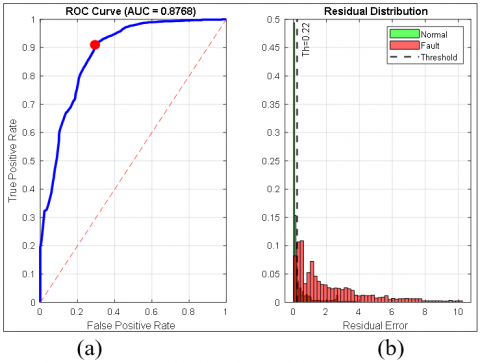
4.3.2 Optimization via ROC analysis (Case study: $T_{J W}$)
The Warning Threshold is designed to detect incipient faults as early as possible. For the representative case of Jacket Water Temperature ($T_{J W}$): An ROC analysis [22] was conducted on the validation dataset (Figure 7). The Youden’s Index maximization identified the theoretical detection limit at 0.22℃. However, relying solely on this statistical limit is impractical due to sensor drift. Therefore, we incorporated the standard industrial thermocouple uncertainty ($\epsilon_{{sensor }} \approx 0.8^{\circ} \mathrm{C}$). The Warning Threshold is calculated as:
$T_{{warn }}=T_{R O C}+\epsilon_{{sensor }}+$ mar. $\approx 0.22+0.8+0.18=1.2^{\circ} \mathrm{C}$ (25)
This value ensures that a warning is triggered only when the deviation exceeds both the algorithm's noise floor and the sensor's physical error margin.
4.3.3 Determination of Alarm Threshold
The Alarm Threshold, which triggers critical safety actions, must be robust against severe external disturbances to prevent false shutdowns.
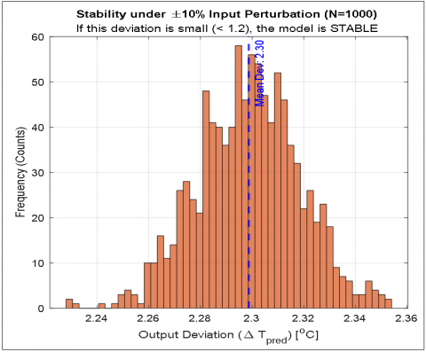
To determine this limit, a Monte Carlo simulation (N = 1000) was conducted with random input perturbations of $\pm 10 \%$. The stability results (Figure 8) indicate that under worst-case disturbance scenarios (simulating rough sea states), the model's output deviation can reach up to 2.30℃.
Consequently, the Alarm Threshold must be set significantly above this worst-case induced deviation:
$T_{{alarm }}>\text{Max Deviation}_{ {MonteCarlo }} (\text{i.e.}, \left.>2.30^{\circ} \mathrm{C}\right)$ (26)
Based on this, a safety value of 4.5℃ was selected. This ensures that the system remains stable during heavy maneuvering and only triggers an alarm when a definitive thermal breakdown occurs.
Applying this adaptive logic to the entire sensor suite, the optimized Warning and Alarm thresholds for all five DIs are summarized in Table 7. These values represent a scientifically calculated balance between sensitivity and robustness.
Table 7. Finalized diagnostic thresholds derived from the calibration phase
|
ID |
Diagnostic Indicator |
Metric Type |
Warning Threshold |
Alarm Threshold |
Physical Basis |
|
DI1 |
EGT Deviation |
Max Deviation |
> 5.5℃ |
> 13℃ |
Based on thermocouple Type-K uncertainty ($\pm 2.2^{\circ} \mathrm{C}$) + combustion noise. |
|
DI2 |
LO Pressure |
Residual (RLO) |
< −0.25 bar |
< −0.6 bar |
Based on pressure transmitter accuracy (±0.05 bar) + Pump ripple. |
|
DI3 |
JW Temperature |
Residual (RJW) |
> 1.2℃ |
> 4.5℃ |
Based on RTD/PT100 accuracy ($\pm 0.5^{\circ} \mathrm{C}$). |
|
DI4 |
Governor Stability |
Amplitude (Agov) |
> 5 RPM |
> 12 RPM |
Detection of mechanical hunting vs. normal speed droop. |
|
DI5 |
Air Leakage |
Drop Rate ($\dot{P}$) |
< −0.01 bar/s |
< −0.04 bar/s |
Early detection of boost pressure loss. |
Figure 7. Statistical threshold optimization analysis. (a) Receiver Operating Characteristic (ROC) Curve showing the optimal trade-off between sensitivity and specificity (AUC = 0.87); (b) Prediction residual distribution histogram
Figure 8. Model robustness verification under parameter uncertainty
4.4 Real-time fault detection on edge device
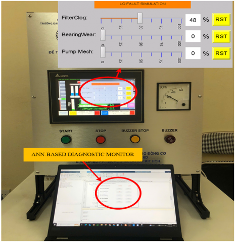
To verify the capability of the integrated system across different physical domains, the diagnostic logic was deployed online using the experimental setup illustrated in Figure 9. The test rig comprises a physical simulation unit equipped with a Delta HMI panel, which allows for the manual injection of faults—such as filter clogging and bearing wear—by adjusting their severity levels (as shown in the detailed inset). Simultaneously, the ANN-based diagnostic monitor operates on a connected workstation to process sensor data in real-time. In this configuration, the MATLAB service queried the SQL Server at 1-second intervals. The validation process was organized into five specific operational scenarios, ranging from normal baseline operation to complex concurrent fault conditions. The detailed experimental design, including the specific fault types and injection severity steps for each scenario, is summarized in Table 8.
4.4.1 Scenario S1: Baseline Validation (Normal Operation)
The engine was operated under healthy conditions at varying speeds (up to 720 RPM) without any fault injection. Throughout this baseline test, all residuals remained within the calibrated safety margins ($|R| \approx 0$), and the Packed_Alarm_Integer returned 0. Consequently, all SCADA indicators remained Green (OFF), confirming the system's stability and the absence of false alarms.
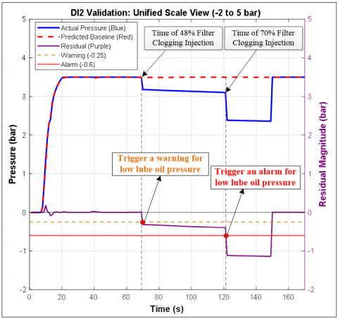
4.4.2 Scenario S2: Hydraulic fault validation (DI2 - Lube Oil Pressure)
To validate the diagnostic response to hydraulic anomalies, a Filter Clogging fault was introduced in two sequential stages. As captured in Figure 9, the fault intensity was manually injected via the HMI touch interface, strictly following the experimental protocol. The corresponding system response is visualized in the data log (Figure 10), highlighting the following behavior:
Table 8. Real-time validation scenarios and fault injection parameters
|
Scenario |
Objective |
Fault Type |
Target Indicator |
Speed Levels |
Injection Severity |
|
S1 |
Baseline Validation |
None (Normal) |
All DIs |
1 ÷ 7 |
0% |
|
S2 |
Hydraulic Response |
Filter Clogging |
DI2 (PLO) |
2 |
48% / 70% |
|
S3 |
Thermal Response |
Radiator Fouling |
DI3 (TJW) |
6 |
45% / 85% |
|
S4 |
Pneumatic Response |
Valve Leakage |
DI5 (PAIR) |
0 |
20% / 60% |
|
S5 |
Concurrent Handling |
Multi-Fault (S2+ S4) |
DI2 & DI5 |
2 |
48% & 60% |
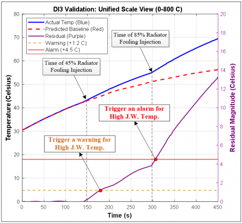
4.4.3 Scenario S3: Thermal fault validation (DI3 - Jacket Water Temperature)
To assess the thermal diagnostic capabilities, a Radiator Fouling condition was simulated. As depicted in Figure 11, the system response was analyzed under two progressive severity levels:
Figure 9. Manual fault injection via HMI: Setting 'Filter Clogging' severity to 48%
Figure 10. Real-time validation of DI2
Figure 11. Real-time validation of DI3
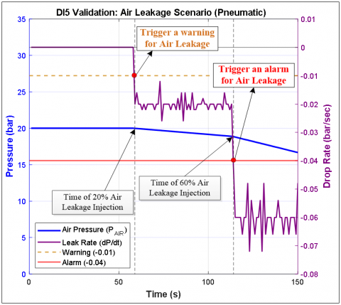
4.4.4 Scenario S4: Pneumatic fault validation (DI5 - Air Leakage)
With the engine in the Stopped State, a Valve Leakage was simulated at two severity levels (20% and 60%). Figure 12 validates the rule-based logic.
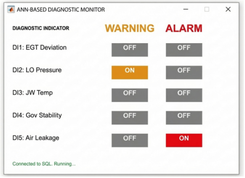
4.4.5 Scenario S5: Concurrent fault handling (System Integration)
Finally, to stress-test the system's isolation capability, both Hydraulic (S2 at 48%) and Pneumatic (S4 at 60%) faults were injected simultaneously.
As shown in the interface screenshot (Figure 13), the system correctly identified and isolated both anomalies. The Status Indicators for DI2 (LO Pressure) and DI5 (Air Leakage) are active (ON/Red), while other subsystems (DI1, DI3, DI4) remain Normal (OFF). This confirms that the diagnostic logic for each subsystem operates independently without cross-interference.
Figure 12. Real-time validation of DI5
Figure 13. Full GUI screenshot showing concurrent alarms
This study successfully developed and validated a low-cost HIL framework to bridge the data scarcity gap in marine engine diagnostics. By integrating a Siemens S7-1200 PLC with a Python-based Edge IPC, the proposed system effectively emulates the thermodynamic behaviors of a Daihatsu 6PSHTb-26D engine, facilitating the safe injection of critical faults (e.g., cooling failures, lubrication degradation) without risking physical assets.
The key contributions and findings are summarized as follows:
Future Work: Despite these promising results, the current validation relies on laboratory and simulation data ("Source Domain"). The next phase of research will focus on bridging the Sim-to-Real gap. Specifically, we aim to collect extensive sea-trial data from operating vessels under varying load conditions. To address the inevitable distribution shift between the HIL simulation and the stochastic marine environment, Domain Adaptation techniques such as Maximum Mean Discrepancy (MMD) [23] will be applied. Furthermore, Transfer Learning strategies, including freezing the early feature-extraction layers and fine-tuning the fully connected layers [24], will be investigated to adapt the pre-trained model to specific individual engines.
This research is funded by Vietnam Maritime University.
[1] Cheliotis, M., Lazakis, I., Theotokatos, G. (2020). Machine learning and data-driven fault detection for ship systems operations. Ocean Engineering, 216: 107968. https://doi.org/10.1016/j.oceaneng.2020.107968
[2] Ma, A., Zhang, J., Shen, H., Cao, Y., Xu, H., Liu, J. (2025). Research on fault diagnosis of marine diesel engines based on CNN-TCN–ATTENTION. Applied Sciences, 15(3): 1651. doi:https://doi.org/10.3390/app15031651
[3] Zhang, J., Pei, G., Zhu, X., Gou, X., et al. (2024). Diesel engine fault diagnosis for multiple industrial scenarios based on transfer learning. Measurement, 228: 114338. https://doi.org/10.1016/j.measurement.2024.114338
[4] Guo, Y., Zhang, J. (2023). Fault diagnosis of marine diesel engines under partial set and cross working conditions based on transfer learning. Journal of Marine Science and Engineering, 11(8): 1527. https://doi.org/10.3390/jmse11081527
[5] Altosole, M., Balsamo, F., Acanfora, M., Mocerino, L., Campora, U., Perra, F. (2022). A digital twin approach to the diagnostic analysis of a marine diesel engine. In Technology and Science for the Ships of the Future, pp. 198-206. https://doi.org/10.3233/PMST220025
[6] Xu, N., Zhang, G., Yang, L., Shen, Z., Xu, M., Chang, L. (2022). Research on thermoeconomic fault diagnosis for marine low speed two stroke diesel engine. Mathematical Biosciences and Engineering, 19(6): 5393-5408. https://doi.org/10.3934/mbe.2022253
[7] Zhou, J., Ouyang, G., Wang, M. (2010). Hardware-in-the-Loop testing of electronically-controlled common-rail systems for marine diesel engine. In 2010 International Conference on Intelligent Computation Technology and Automation, Changsha, China, pp. 421-424. https://doi.org/10.1109/ICICTA.2010.40
[8] Kadhum, L.M., Mohammed, S.J., Al-Gayem, Q. (2025). Advanced SCADA-PLC S7-1200 communication system for aeration unit in wastewater treatment stations. Journal Européen des Systèmes Automatisés, 58(4): 747-754. https://doi.org/10.18280/jesa.580408
[9] Pulkrabek, W.W. (2004). Engineering Fundamentals of the Internal Combustion Engine (2nd ed.). Pearson Prentice Hall.
[10] Heywood, J.B. (2018). Internal Combustion Engine Fundamentals (2nd ed.). McGraw-Hill Education.
[11] Ferguson, C.R., Kirkpatrick, A.T. (2015). Internal Combustion Engines: Applied Thermosciences (3rd ed.). John Wiley & Sons.
[12] Guzzella, L., Onder, C.H. (2010). Introduction to Modeling and Control of Internal Combustion Engines (2nd ed.). Springer-Verlag.
[13] White, F.M. (2015). Fluid Mechanics (8th ed.). McGraw-Hill Education.
[14] Ogata, K. (2010). Modern Control Engineering (5th ed.). Prentice Hall.
[15] McGeorge, H.D. (1998). Marine Auxiliary Machinery (7th ed.). Butterworth-Heinemann.
[16] Woodyard, D. (2009). Pounder’s Marine Diesel Engines and Gas Turbines (9th ed.). Butterworth-Heinemann.
[17] Taylor, D.A. (1996). Introduction to Marine Engineering (2nd ed.). Butterworth-Heinemann.
[18] Andrade, E. (1930). The viscosity of liquids. Nature, 125: 309-310. http://doi.org/10.1038/125309b0
[19] Mahmood, M.S., Shareef, I.R. (2024). Applications of artificial intelligence for smart conveyor belt monitoring systems: A comprehensive review. Journal Européen des Systèmes Automatisés, 57(4): 1195-1206. https://doi.org/10.18280/jesa.570426
[20] Co, D.D.M., Ltd. (1981). Instruction Manual for Daihatsu Diesel Engine Model PS-26.
[21] Montgomery, D.C. (2019). Introduction to Statistical Quality Control (8th ed.). John Wiley & Sons.
[22] Fawcett, T. (2006). An introduction to ROC analysis. Pattern Recognition Letters, 27(8): 861-874. https://doi.org/10.1016/j.patrec.2005.10.010
[23] Gretton, A., Borgwardt, K.M., Rasch, M.J., Schölkopf, B., Smola, A. (2012). A kernel two-sample test. The Journal of Machine Learning Research, 13(1): 723-773. https://dl.acm.org/doi/abs/10.5555/2188385.2188410.
[24] Pan, S.J., Yang, Q. (2009). A survey on transfer learning. IEEE Transactions on Knowledge and Data Engineering, 22(10): 1345-1359. https://doi.org/10.1109/TKDE.2009.191