Chetioui Lotfi![]() | Achouri Mourad
| Achouri Mourad![]() | Youcef Zennir
| Youcef Zennir![]() | Mohamed Benghanem*
| Mohamed Benghanem*![]() | Adel Ashour
| Adel Ashour![]()
© 2026 The authors. This article is published by IIETA and is licensed under the CC BY 4.0 license (http://creativecommons.org/licenses/by/4.0/).
OPEN ACCESS
In modern control engineering, the demand for robust and adaptive control strategies is critical for managing complex, nonlinear, and uncertain systems. This paper investigates sliding mode control (SMC) and fuzzy PID control applied to a doubly fed induction generator (DFIG), two advanced techniques widely used in both industrial and academic contexts. SMC is known for its high robustness and finite-time convergence; however, it suffers from chattering and dependence on accurate system modeling. In contrast, the fuzzy PID controller combines the classical PID structure with fuzzy logic to provide adaptive and smooth control without requiring a precise mathematical model. Through theoretical analysis and a review of recent research findings, this study highlights the strengths and limitations of each method in terms of robustness, adaptability, implementation complexity, and application suitability. The results indicate that while SMC excels in robustness and precision, the fuzzy PID controller offers a more flexible and user-friendly alternative for systems with nonlinear or uncertain dynamics. Ultimately, the choice between the proposed methods depends on the specific requirements of the target application, with future research opportunities lying in hybrid strategies that combine the robustness of SMC with the adaptability of fuzzy PID control to enhance performance in renewable energy systems.
sliding mode control, doubly fed induction generator, stability, fuzzy logic, fuzzy PID controller
Due to the increasing economic and environmental costs of fossil fuels, along with the global push to replace them, the energy landscape has undergone significant changes in recent decades. Renewable energy sources have emerged as a key solution to these challenges, helping to meet growing energy demands while also mitigating the looming energy crisis [1]. Among renewable technologies, wind energy has become a leading option due to its abundance, environmental benefits, and rapid global expansion [2, 3].
At the same time, a significant portion of electrical energy is transformed into mechanical energy using motors. Among these, doubly fed induction generator (DFIG) is especially popular in industrial applications due to its suitability for variable-speed operations, namely in electric vehicles, wind turbine systems, and marine propulsion. The doubly-fed induction machine (DFIM) offers several advantages, including the following [4-7]: The DFIG can be supplied and controlled through the stator, rotor, or a combination of both; it is capable of operating over a wide range of speed variations around the synchronous speed (up to ± 30%), enabling maximum power generation at varying wind speeds in turbine systems; it permits decoupled regulation of reactive and active power; and it enables independent control of flux, torque, and power factor.
In the field of control systems, the challenges associated with nonlinear and uncertain processes remain a key priority. Classical methods, such as PID control, have been widely used because of their efficiency and simplicity, especially for linear systems. However, when dealing with highly nonlinear, time-varying, or uncertain systems, such as those found in magnetohydrodynamic flows [8], more advanced control strategies are required. Lotfi et al. [9, 10] optimized the PID controller using metaheuristic algorithms applied to the speed control of a WECS and DFIM. Larabi et al. [11] applied an LQG-based LMI technique to a doubly-fed induction generator (BDFIG). Arabi et al. [12] proposed a nonlinear PI regulator enhanced by meta-heuristic methods for wind turbine speed regulation.
Two such strategies are sliding mode control (SMC) and the fuzzy PID controller.
SMC is a widely used control method due to its efficiency and robustness. The SMC control law is designed using the system model and consists of two distinct components. The first is the equivalent control, which forces the system dynamics to reach the selected sliding surface, ensuring convergence. The second is called the switching term; it keeps the system states on the sliding surface once it is reached. This control scheme has been applied in various studies to manage a wide range of systems, including robotic systems [13], magnetic levitation (MAGLEV) systems [14], and permanent magnet synchronous motors (PMSMs) [15].
In recent years, numerous studies have proposed and implemented advanced control strategies for DFIGs. Karakasis et al. [16] developed a comprehensive control scheme based on maximum power point tracking (MPPT) and loss minimization (LM) for wind systems equipped with DFIGs, aiming to maximize electrical energy production. Bouderbala et al. [17] introduced both direct and indirect field-oriented control (FOC) methods to enhance the reactive and active power outputs of DFIGs connected to variable-speed wind turbines. Jeon et al. [18] proposed a proportional–integral (PI) controller for frequency smoothing in DFIGs. Sadeghi et al. [19] applied a super-twisting sliding mode control technique combined with direct power control (DPC) to brushless doubly-fed induction generators (BDFIGs).
Their approach addressed the drawbacks of conventional DPC, such as power ripples and current distortion, while improving robustness compared to vector control. El Ouanjli et al. [20] introduced fuzzy direct torque control (FDTC) for doubly-fed induction machines (DFIMs) equipped with two voltage source inverters (VSIs), focusing on reducing electromagnetic torque ripples and improving total harmonic distortion (THD). Benbouhenni and Bizon [21] applied direct vector control to extract optimal active and reactive power from dual-rotor wind power (DRWP) systems using DFIGs. Their approach involved rotor current control through four-level fuzzy pulse-width modulation (PWM) and replaced the conventional PI controller with a neural network. To address the drawbacks of field-oriented control, namely significant torque and flux oscillations, Ayrir et al. [22] proposed a fuzzy direct torque regulation method for DFIG-based wind turbines. Tamalouzt et al. [23] implemented a direct reactive power regulation approach using a three-level inverter topology for DFIG-based wind turbines. Xiahou and Wu [24] introduced a fault-tolerant control scheme based on a Kalman filter to handle voltage and current sensor faults in DFIGs. Herizi et al. [25] employed a backstepping control technique enhanced with fuzzy logic to improve the efficiency of DFIG-based systems. Motivated by the above discussion, the present study proposes the application of SMC for controlling the DFIG system. The stability of the applied controller is established with the help of a Lyapunov function. The performance of SMC is compared with that of a fuzzy PID controller, focusing on key parameters, namely overshoot, rise time, and steady-state error. The models are simulated using Simscape in MATLAB/Simulink. The simulation results demonstrate that SMC outperforms the fuzzy PID controller in terms of rise time and steady-state error.
The layout of the paper is as follows: Section 2 presents the dynamics of DFIG. Section 3 discusses the design and system stability of the implemented approach. Section 4 provides the application of fuzzy PID on DFIG, and Section 5 interprets the simulation results along with a detailed discussion. Finally, Section 6 concludes the paper with the main findings.
The DFIGs dynamics in d-q frame are given by:
Electrical equations:
$\left\{\begin{array}{c}\mathrm{v}_{\mathrm{ds}}=\mathrm{R}_{\mathrm{s}} \mathrm{i}_{\mathrm{ds}}+\frac{\mathrm{d}}{\mathrm{dt}} \varphi_{\mathrm{ds}}-\mathrm{W}_{\mathrm{s}} \varphi_{\mathrm{qs}} \\ \mathrm{v}_{\mathrm{qs}}=\mathrm{R}_{\mathrm{s}} \mathrm{i}_{\mathrm{qs}}+\frac{\mathrm{d}}{\mathrm{dt}} \varphi_{\mathrm{qs}}+\mathrm{W}_{\mathrm{s}} \varphi_{\mathrm{ds}} \\ \mathrm{v}_{\mathrm{dr}}=\mathrm{R}_{\mathrm{r}} \mathrm{i}_{\mathrm{dr}}+\frac{\mathrm{d}}{\mathrm{dt}} \varphi_{\mathrm{dr}}-\mathrm{W}_{\mathrm{r}} \varphi_{\mathrm{qr}} \\ \mathrm{v}_{\mathrm{qr}}=\mathrm{R}_{\mathrm{r}} \mathrm{i}_{\mathrm{qr}}+\frac{\mathrm{d}}{\mathrm{dt}} \varphi_{\mathrm{qr}}+\mathrm{w}_{\mathrm{r}} \varphi_{\mathrm{ds}}\end{array}\right.$ (1)
Stator and rotor flux equations:
$\left\{\begin{array}{l}\varphi_{\mathrm{ds}}=\mathrm{L}_{\mathrm{s}} \mathrm{i}_{\mathrm{ds}}+\mathrm{Mi}_{\mathrm{dr}} \\ \varphi_{\mathrm{qs}}=\mathrm{L}_{\mathrm{s}} \mathrm{i}_{\mathrm{qs}}+\mathrm{Mi}_{\mathrm{qr}} \\ \varphi_{\mathrm{dr}}=\mathrm{L}_{\mathrm{r}} \mathrm{i}_{\mathrm{dr}}+\mathrm{Mi}_{\mathrm{ds}} \\ \varphi_{\mathrm{qr}}=\mathrm{L}_{\mathrm{r}} \mathrm{i}_{\mathrm{qr}}+\mathrm{Mi}_{\mathrm{qs}}\end{array}\right.$ (2)
$\dot{\Omega}=-\frac{P M}{J L_s} i_{q r} \varphi_{d s}-\frac{f}{j} \Omega$ (3)
where,
$\mathrm{v}_{\mathrm{ds}}, \mathrm{v}_{\mathrm{qs}}$: Voltages of stator in the d-q reference frame.
$\mathrm{v}_{\mathrm{dr}}, \mathrm{v}_{\mathrm{qr}}$: Rotor voltages in the d-q axis.
$\mathrm{i}_{\mathrm{ds}}, \mathrm{i}_{\mathrm{qs}}$: Currents of the stator in the d-q axis.
$\mathrm{i}_{\mathrm{dr}}, \mathrm{i}_{\mathrm{qr}}$: Currents of rotor in the d-q axis.
$\mathrm{L}_{\mathrm{s}}, \mathrm{L}_{\mathrm{r}}, \mathrm{M}$: Stators mutual, self-inductances, and the windings of the rotor, respectively.
$\mathrm{R}_{\mathrm{s}}, \mathrm{R}_{\mathrm{r}}$: the stator and rotor resistance.
$\varphi_{\mathrm{ds}}, \varphi_{\mathrm{qs}}$: stator flux linkages in d-q axis reference.
$\varphi_{\mathrm{dr}}, \varphi_{\mathrm{qr}}$: rotor flux linkages in d-q frame.
$\Omega$: is a speed.
$f$: indicate the friction coefficient.
$J$: represents the moment of inertia.
In the following, it is demonstrated that the control objectives for a DFIG can be achieved by appropriately controlling the rotor currents. By aligning the d-axis of the park transformation with the stator flux, the system equations can be given by:
$\left\{\begin{array}{c}\varphi_{d s}=\varphi_s \\ \varphi_{q s}=0\end{array}\right.$ (4)
where, $\varphi_s$ represent a constant.
Considering that the line voltage amplitude $V_s$ and the synchronous speed $w_s$ remain constant, the stator flux $\varphi_{\mathrm{ds}}=\varphi_{\mathrm{s}}$. Neglecting the stator resistance is a reasonable choice for machines applied in wind turbine in the case of high-power. The equations of stator voltage are given as follows:
$\left\{\begin{array}{c}\mathrm{v}_{\mathrm{ds}}=0 \\ \mathrm{v}_{\mathrm{qs}}=\mathrm{V}_{\mathrm{s}}=\mathrm{w}_{\mathrm{s}} \varphi_{\mathrm{s}}\end{array}\right.$ (5)
Based on Eqs. (19) and (24), the currents of the stator are algebraically associated to the currents of rotor by the following expressions:
$\left\{\begin{array}{c}\mathrm{i}_{\mathrm{ds}}={-\frac{\mathrm{M}}{\mathrm{L}_{\mathrm{s}}} \mathrm{i}}_{dr}+\frac{\varphi_{\mathrm{s}}}{\mathrm{L}_{\mathrm{s}}} \\ \mathrm{i}_{\mathrm{qs}}=-\frac{\mathrm{M}}{\mathrm{L}_{\mathrm{s}}} \mathrm{i}_{\mathrm{qr}}\end{array}\right.$ (6)
Taking the above considerations into account, the reduced-order electrical model can be derived, in which the rotor currents serve as the primary variables and the stator currents are algebraically related to them.
$\left\{\begin{array}{c}\frac{d i_{d r}}{d t}=\frac{1}{L_r \sigma}\left(v_{d r}-R_r i_{d r}+L_r\left(w_s-w\right) \sigma i_{q r}\right) \\ \frac{d i_{q r}}{d t}=\frac{1}{L_r \sigma}\left(v_{q r}-R_r i_{q r}+L_r\left(w_s-w\right) \sigma i_{d r}-\frac{M}{L_s}\left(w_s-w\right) \varphi_{d s}\right)\end{array}\right.$ (7)
SMC is a popular control method designed using two control terms. The first is the equivalent control, which drives the system dynamics to converge to the selected tracking errors (sliding surface). The second is the switching control, which maintains the system dynamics along the chosen sliding surface [26, 27]. The need for such robust stability guarantees is a recurring theme in engineering systems, as highlighted by recent reviews leveraging computational intelligence for stability analysis in other complex domains [28].
Table 1 summarizes the control objectives of this study.
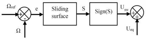
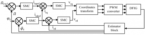
Figures 1 and 2 illustrate the control architecture of the proposed approach.
Table 1. The control objective
|
Commands |
Objectives |
|
$\mathrm{i}_{\mathrm{dr}}=\mathrm{i}_{\mathrm{drref}}$ |
$\Omega=\Omega_{\mathrm{ref}}$ |
|
$\mathrm{i}_{\mathrm{qr}}=\mathrm{i}_{\mathrm{qrref}}$ |
/ |
Figure 1. Sliding mode control diagram
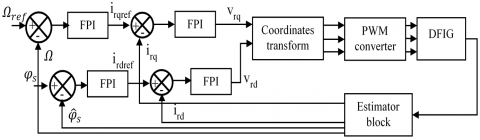
Figure 2. Sliding mode control (SMC) based doubly fed induction generator (DFIG) control diagram
3.1 Speed controller design
The sliding surface is expressed by:
$\mathrm{s}_1=\mathrm{e}_1=\Omega_{\mathrm{ref}}-\Omega$ (8)
Differentiating the above tracking error yields:
$\dot{\mathrm{s}}_1=\frac{\mathrm{d} \Omega_{\mathrm{ref}}}{\mathrm{dt}}-\frac{\mathrm{d} \Omega}{\mathrm{dt}}$ (9)
After substituting Eq. (3) into Eq. (9), we get:
$\dot{\mathrm{s}}_1=\frac{\mathrm{d} \Omega_{\mathrm{ref}}}{\mathrm{dt}}-\left(-\frac{\mathrm{PM}}{\mathrm{JL}_{\mathrm{s}}} \mathrm{i}_{\mathrm{qr}} \varphi_{\mathrm{ds}}-\frac{\mathrm{f}}{\mathrm{j}} \Omega\right)$ (10)
Considering the definition of SMC, the equivalent and switching controls can be expressed as:
$\mathrm{i}_{\mathrm{qre}}^{\mathrm{eq}}=-\frac{\mathrm{JL}_{\mathrm{s}}}{\mathrm{PM} \varphi_{\mathrm{ds}}}\left(\dot{\Omega}_{\mathrm{ref}}+\frac{\mathrm{f}}{\mathrm{j}} \Omega\right)$ (11)
$\mathrm{i}_{\mathrm{qre}}^{\mathrm{sw}}=\rho_1 \operatorname{sign}\left(\mathrm{~s}_1\right)$ (12)
3.2 Current controller design
To establish the current control law, the following sliding surfaces are selected:
$\mathrm{s}_2=\mathrm{e}_2=\mathrm{i}_{\mathrm{drref}}-\mathrm{i}_{\mathrm{dr}}$ (13)
$\mathrm{s}_3=\mathrm{e}_3=\mathrm{i}_{\mathrm{qrref}}-\mathrm{i}_{\mathrm{qr}}$ (14)
The time derivatives of Eqs. (13) and (14) are calculated as follows:
$\dot{\mathrm{s}}_2=\frac{\mathrm{di}_{\mathrm{drref}}}{\mathrm{dt}}-\frac{\mathrm{di}_{\mathrm{dr}}}{\mathrm{dt}}$ (15)
$\dot{\mathrm{s}}_3=\frac{\mathrm{di}_{\mathrm{qrref}}}{\mathrm{dt}}-\frac{\mathrm{di}_{\mathrm{qr}}}{\mathrm{dt}}$ (16)
By substituting Eq. (7) into Eqs. (15) and (16), we obtain:
$\dot{\mathrm{s}}_2=\frac{\mathrm{di}_{\mathrm{drref}}}{\mathrm{dt}}-\frac{1}{\mathrm{~L}_{\mathrm{r}} \sigma}\left(\mathrm{v}_{\mathrm{dr}}-\mathrm{R}_{\mathrm{r}} \mathrm{i}_{\mathrm{dr}}+\mathrm{L}_{\mathrm{r}}\left(\mathrm{w}_{\mathrm{s}}-\mathrm{w}\right) \sigma \mathrm{i}_{\mathrm{qr}}\right)$ (17)
$\dot{\mathrm{s}}_3=\frac{\mathrm{di}_{\mathrm{qrref}}}{\mathrm{dt}}-\frac{1}{\mathrm{~L}_{\mathrm{r}} \sigma}\left(\mathrm{v}_{\mathrm{qr}}-\mathrm{R}_{\mathrm{r}} \mathrm{i}_{\mathrm{qr}}+\mathrm{L}_{\mathrm{r}}\left(\mathrm{w}_{\mathrm{s}}-\mathrm{w}\right) \sigma \mathrm{i}_{\mathrm{dr}}-\frac{\mathrm{M}}{\mathrm{L}_{\mathrm{s}}}\left(\mathrm{w}_{\mathrm{s}}-\mathrm{w}\right) \varphi_{\mathrm{ds}}\right)$ (18)
As mentioned previously, the equivalent control attempts to drive the system dynamics onto the considered sliding surface, thereby making the latter converge to zero [29-31]. Therefore, the equivalent control laws are given by:
$\mathrm{v}_{\mathrm{dr}}^{\mathrm{eq}}=\mathrm{L}_{\mathrm{r}} \sigma\left(\left(\mathrm{R}_{\mathrm{r}} \mathrm{i}_{\mathrm{qr}}-\mathrm{L}_{\mathrm{r}}\left(\mathrm{w}_{\mathrm{s}}-\mathrm{w}\right) \sigma \mathrm{i}_{\mathrm{dr}}\right)-\frac{\mathrm{di}_{\mathrm{drref}}}{\mathrm{dt}}\right)$ (19)
$\mathrm{v}_{\mathrm{qr}}^{\mathrm{eq}}=\mathrm{L}_{\mathrm{r}} \sigma\left(\left(\mathrm{R}_{\mathrm{r}} \mathrm{i}_{\mathrm{dr}}-\mathrm{L}_{\mathrm{r}}\left(\mathrm{w}_{\mathrm{s}}-\mathrm{w}\right) \sigma \mathrm{i}_{\mathrm{qr}}+\frac{\mathrm{M}}{\mathrm{L}_{\mathrm{s}}} \frac{\mathrm{d}}{\mathrm{dt}} \varphi_{\mathrm{ds}}\right)\right)-\frac{\mathrm{di}_{\mathrm{qrref}}}{\mathrm{dt}}$ (20)
In the reaching step, the switching term is used to maintain the system dynamics on the selected sliding surface [31], and it is expressed as:
$\mathrm{v}_{\mathrm{dr}}^{\mathrm{sw}}=\mathrm{L}_{\mathrm{r}} \sigma\left(\rho_1 \operatorname{sgn}\left(\mathrm{~s}_1\right)\right)$ (21)
$\mathrm{v}_{\mathrm{qr}}^{\mathrm{sw}}=\mathrm{L}_{\mathrm{r}} \sigma\left(\rho_2 \operatorname{sgn}\left(\mathrm{~s}_2\right)\right)$ (22)
The final control laws are obtained by adding the equivalent terms to the switching terms.
3.3 Stability analysis
In this paper, the stability of the proposed control laws is established using the following Lyapunov function [32]:
$\mathrm{V}=\sum_{\mathrm{i}=1}^3 \frac{1}{2} \mathrm{~s}_{\mathrm{i}}^2$ (23)
After computing the derivative of Eq. (23), we obtain:
$\dot{\mathrm{V}}=\sum_{\mathrm{i}=1}^3 \mathrm{~s}_{\mathrm{i}} \dot{\mathrm{s}}_{\mathrm{i}}=s_1 \dot{\mathrm{~s}}_1+s_2 \dot{\mathrm{~s}}_2+s_3 \dot{\mathrm{~s}}_3$ (24)
After substituting Eqs. (10), (17), and (18) into Eq. (24), we obtain:
$\begin{gathered}\dot{\mathrm{V}}=s_1\left(\frac{\mathrm{~d} \Omega_{\mathrm{ref}}}{\mathrm{dt}}-\left(-\frac{\mathrm{PM}}{\mathrm{JL}_{\mathrm{s}}} \mathrm{i}_{\mathrm{qr}} \varphi_{\mathrm{ds}}-\frac{\mathrm{f}}{\mathrm{j}} \Omega\right)+\delta_1\right)+s_2\left(\frac{\mathrm{di}_{\mathrm{drref}}}{\mathrm{dt}}-\frac{1}{\mathrm{~L}_{\mathrm{r}} \sigma}\left(\mathrm{v}_{\mathrm{dr}}-\right.\right. \\ \left.\left.\mathrm{R}_{\mathrm{r}} \mathrm{i}_{\mathrm{dr}}+\mathrm{L}_{\mathrm{r}}\left(\mathrm{w}_{\mathrm{s}}-\mathrm{w}\right) \sigma \mathrm{i}_{\mathrm{qr}}\right)+\delta_2\right)+s_3\left(\frac{\mathrm{di}_{\mathrm{qrref}}}{\mathrm{dt}}-\frac{1}{\mathrm{~L}_{\mathrm{r} \sigma}}\left(\mathrm{v}_{\mathrm{qr}}-\right.\right. \\ \left.\left.\mathrm{R}_{\mathrm{r}} \mathrm{i}_{\mathrm{qr}}+\mathrm{L}_{\mathrm{r}}\left(\mathrm{w}_{\mathrm{s}}-\mathrm{w}\right) \sigma \mathrm{i}_{\mathrm{dr}}-\frac{\mathrm{M}}{\mathrm{L}_{\mathrm{s}}}\left(\mathrm{w}_{\mathrm{s}}-\mathrm{w}\right) \varphi_{\mathrm{ds}}\right) \delta_3\right)\end{gathered}$ (25)
where, $\delta_i=\left(\delta_1, \delta_2, \delta_3\right)$ denotes the system uncertainties.
In sliding mode, the control input is given by the sum of the equivalent term and the switching term; therefore, the control law is expressed as:
$\left\{\begin{array}{c}\mathrm{i}_{\mathrm{qr}}=\mathrm{i}_{\mathrm{qr}}^{\mathrm{eq}}+\mathrm{i}_{\mathrm{qr}}^{\mathrm{sw}} \\ \mathrm{v}_{\mathrm{dr}}=\mathrm{v}_{\mathrm{dr}}^{\mathrm{eq}}+\mathrm{v}_{\mathrm{dr}}^{\mathrm{sw}} \\ \mathrm{v}_{\mathrm{qr}}=\mathrm{v}_{\mathrm{qr}}^{\mathrm{eq}}+\mathrm{v}_{\mathrm{qr}}^{\mathrm{sw}}\end{array}\right.$ (26)
where, $\mathrm{i}_{\mathrm{qr}}^{\mathrm{eq}}, \mathrm{i}_{\mathrm{qr}}^{\mathrm{sw}}, \mathrm{v}_{\mathrm{dr}}^{\mathrm{eq}}, \mathrm{v}_{\mathrm{dr}}^{\mathrm{sw}}, \mathrm{v}_{\mathrm{qr}}^{\mathrm{eq}}$ and $\mathrm{v}_{\mathrm{qr}}^{\mathrm{sw}}$ are given in Eqs. (11) and (12) and Eqs. (19)-(22).
Substituting Eq. (25) into Eq. (24) yields:
$\begin{gathered}\dot{\mathrm{V}}=\mathrm{s}_1\left(-\rho_1 \operatorname{sgn}\left(\mathrm{~s}_1\right)+\delta_1\right)+\mathrm{s}_2\left(-\rho_2 \operatorname{sgn}\left(\mathrm{~s}_2\right)+\delta_2\right) +\mathrm{s}_3\left(-\rho_3 \operatorname{sgn}\left(\mathrm{~s}_3\right)+\delta_3\right)\end{gathered}$ (27)
Eq. (27) can be rewritten as follows:
$\dot{\mathrm{V}}=\sum_{\mathrm{i}=1}^3\left(-\rho_{\mathrm{i}}\left|\mathrm{s}_{\mathrm{i}}\right|+\mathrm{s}_{\mathrm{i}} \delta_i\right)$ (28)
After selecting $\rho_{\mathrm{I}}>\max \left(\delta_{\mathrm{i}}\right)$, we have $\dot{V}<0$. Since $\mathrm{V}>0$ and $\dot{V}<0$, the system’s states are guaranteed to converge toward the selected sliding surface, thereby achieving the specified steady state in finite time.
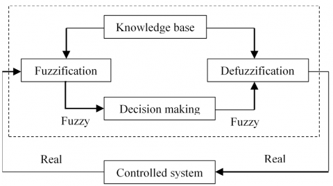
This work uses a fuzzy logic controller (FLC) to develop a novel control strategy. The advantages of FLC over traditional controllers include its ability to function effectively even in the absence of an accurate mathematical model [33, 34]. This adaptability makes it a popular choice for complex systems, as recently demonstrated in its successful application to motor control in renewable energy systems [35]. The fuzzy controller consists of three main components: the fuzzy rule set, the fuzzy base rules, and the fuzzification process. Its main feature is the use of linguistic variables instead of numerical ones. The fuzzy logic control technique is inspired by the human ability to understand and interpret the behavior of complex systems by constructing a set of qualitative rules. FLC offers a straightforward method for reaching conclusions from imprecise, ambiguous, noisy, or incomplete input data [33, 34]. The steps of the FLC are illustrated in Figure 3.
Figure 3. Fuzzy logic diagram
In Figure 3, input data are converted into suitable linguistic values by the fuzzification interface. The knowledge base comprises a database, a set of control rules, and key linguistic definitions. A decision is made based on the descriptions of the linguistic variables and the control rule data. An interface for defuzzification then converts the fuzzy control input into a crisp (numerical) control output. The implementation of the fuzzy inference system (FIS) for diagnosis involves three functional stages, as illustrated in Figure 3.
4.1 Step of fuzzification
Fuzzification consists of determining the fuzzy sets for both the inputs and outputs. The interval, the number of fuzzy sets, and the shape of the membership functions must all be known beforehand.
4.2 Inference step
At this point, we create the fuzzy rules that determine the output based on the input variable values. The operator then generates an implication from each rule, consisting of premises connected by AND or OR. After defuzzification [33, 34], the aggregation of these rules results in a single, uniform output value for the variable.
4.3 Defuzzification stage
In this step, the FIS’s linguistic variable output is converted into a numerical value. There are three primary defuzzification methods: the maximum method, which corresponds to the minimum horizontal coordinate of the output membership function [36, 37] and is rarely used; the weighted average method; and the centroid method, which is the most effective. The centroid method calculates the center of gravity of the output membership function and is applied in the present work. The FLC receives two input signals: the speed error and the error variation. Defuzzification using the centroid method produces the FLC output [37, 38].
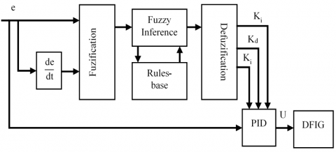
To tune the PID gains using FLC, two inputs are selected: the error and the rate of error. The outputs of the FLC are Kp, Ki and Kd. Seven membership functions are used for both inputs and outputs. Seven linguistic variables are assigned for the inputs (BN: big negative, MN: medium negative, N: negative, ZE: zero, P: positive, MP: medium positive, and BP: big positive) and seven others for the outputs (EM: extremly marginal, VM: very marginal, M: marginal, A: avereage, H: hight, VH: very hight, and EH: extremly hight). Tables 2, 3 and 4 show the parameters of the inputs and outputs of the FLC and the fired fuzzy rules.
Table 2. The parameters of inputs and outputs of fuzzy logic controller (FLC)
|
Variables |
Range |
Number of Membership Functions |
Type of Membership Functions |
|
Error |
[-1 1] |
7 |
Triangular |
|
Error rate |
[-1 1] |
7 |
Triangular |
|
Kp |
[2286 3302] |
7 |
Gaussian |
|
Ki |
[22860 33020] |
7 |
Gaussian |
Table 3. Fuzzy inferences for determining Kd [39]
|
e Δe |
BN |
MN |
N |
ZE |
P |
MP |
BP |
|
BN |
A |
H |
VH |
EH |
VH |
H |
A |
|
MN |
M |
A |
H |
VH |
H |
A |
M |
|
N |
VM |
M |
A |
H |
A |
M |
VM |
|
ZE |
EM |
VM |
M |
A |
M |
VM |
EM |
|
P |
VM |
M |
A |
H |
A |
M |
VM |
|
MP |
M |
A |
H |
VH |
H |
A |
M |
|
BP |
A |
H |
VH |
EB |
VH |
H |
A |
Table 4. Fuzzy inferences for determining Ki and Kp [39]
|
e Δe |
BN |
MN |
N |
ZE |
P |
MP |
BP |
|
BN |
A |
M |
VM |
EM |
VM |
M |
A |
|
MN |
H |
A |
M |
VM |
M |
A |
H |
|
N |
VH |
H |
A |
M |
A |
H |
VH |
|
ZE |
EH |
VH |
H |
A |
H |
VH |
EH |
|
P |
VH |
H |
A |
M |
A |
H |
VH |
|
MP |
H |
A |
M |
VM |
M |
A |
H |
|
BP |
A |
M |
VM |
EM |
VM |
M |
A |
Figures 4 and 5 depict the proposed control diagram for DFIG regulation.
Figure 4. The control loop of fuzzy PID
Figure 5. The control loop of fuzzy PID based DFIG
The results presented in this study were obtained using MATLAB/Simulink. To compare the performance of the proposed approach, a fuzzy PID controller was considered. The results obtained using the applied control strategies are illustrated in Figures 6-11.

Figure 6. The DFIG’s speed obtained by SMC

Figure 7. The rotor current $\left(\mathrm{i}_{\mathrm{rd}}\right)$ obtained by SMC

Figure 8. The rotor current $\left(\mathrm{i}_{\mathrm{rq}}\right)$ obtained by SMC

Figure 9. The DFIG’s speed obtained by FLC PID

Figure 10. The rotor current $\left(\mathrm{i}_{\mathrm{rd}}\right)$ obtained by FLC PID

Figure 11. The rotor current $\left(\mathrm{i}_{\mathrm{rq}}\right)$ obtained by FLC PID
The machine and controller parameters are listed in Tables 5 and 6. The controller parameters were determined using a trial-and-error approach.
Figures 6-8 present the results for the rotor speed and rotor currents (ird and irq) obtained using the SMC controller. The figures show that the DFIG rotor speed and currents converge rapidly and accurately to their respective reference values.
Figures 9-11 show the rotor speed and rotor currents (ird and irq) of the DFIG obtained using the Fuzzy–PID controller. From the figures, it can be observed that the Fuzzy–PID controller achieves high tracking performance.
To evaluate the tracking performance of the proposed controller, overshoot, rise time, and steady-state error were considered. The performance of the applied controllers is reported in Table 7.
Table 5. The DFIG’s parameters
|
Parameters |
Value |
|
Stator resistance |
2.6.10-3Ω |
|
Rotor resistance |
2.9.10-3Ω |
|
Stator inductance |
0.0026H |
|
Rotor inductance |
0.0026H |
|
Mutual inductance |
2.5.10-3H |
|
Pole pairs |
2 |
|
Grid frequency |
50HZ |
|
Total damping |
0.003 |
|
Total inertia |
127 kg m2 |
Table 6. The controller’s parameters
|
Value |
Speed Control |
Current Control iq |
Current Control id |
|
$\rho_1$ |
150 |
/ |
/ |
|
$\rho_2$ |
/ |
150 |
/ |
|
$\rho_3$ |
/ |
/ |
150 |
Table 7. The performance of the employed controllers
|
Performances |
SMC |
Fuzzy PID |
|
Overshoot |
0.31 |
0.031 |
|
Rising time |
0.328s |
1.874s |
|
Steady error |
0.002 |
0.0074 |
Table 4 summarizes the tracking performance of the applied controllers. The fuzzy PID controller exhibits lower overshoot, whereas the SMC controller achieves superior steady-state error and rise time.
The above comparative analysis shows that the fuzzy PID controller yields a lower overshoot, which reduces mechanical stress on components (thereby improving the safety of elements such as blades), provides more stable power, and enhances grid stability. Similarly, the results demonstrate that the SMC offers better accuracy, meaning that the wind turbine operates closer to its theoretical maximum power, ensuring improved performance. Therefore, the choice between the proposed control strategies should be determined based on the trade-off between safety and efficiency.
This paper presented a comparative analysis of SMC and fuzzy PID control for the speed regulation of a DFIG. The proposed SMC approach, supported by Lyapunov-based stability analysis, demonstrated high robustness against internal parameter variations and external disturbances while ensuring fast and stable closed-loop dynamics. Simulation results confirmed that SMC achieves superior rise time and lower steady-state error compared to the fuzzy PID controller, making it particularly effective in scenarios where precision and dynamic response are critical. Conversely, the fuzzy PID controller exhibited reduced overshoot, highlighting its ability to provide smoother transient behavior and easier implementation in systems with model uncertainties. The pros and cons of both presented schemes are listed in Table 8.
Table 8. The controller’s parameters
|
Control Techniques |
SMC |
Fuzzy PID |
|
Robustness |
good |
Middle |
|
System modeling |
Required |
Not required |
|
Controller design |
Complicated |
Middle |
|
Expert knowledge |
Not required |
Required |
|
Stability proof |
Yes |
No |
|
Computation loading |
Light |
Heavy |
Overall, the study shows that SMC is well-suited for high-performance control of DFIG-based renewable energy systems, whereas fuzzy PID remains an attractive option when simplicity, flexibility, and lower overshoot are prioritized. These findings underline the importance of selecting a control strategy based on specific application requirements, such as response speed, robustness, and implementation complexity.
Future research may extend this work by comparing the presented approaches with other advanced controllers, namely the linear quadratic regulator (LQR) and model predictive controller (MPC).
[1] Valipour, M. (2015). Future of agricultural water management in Africa. Archives of Agronomy and Soil Science, 61(7): 907-927. https://doi.org/10.1080/03650340.2014.961433
[2] Li, L., Liang, Y., Niu, J., He, J., et al. (2023). The fault ride-through characteristics of a double-fed induction generator using a dynamic voltage restorer with superconducting magnetic energy storage. Applied Sciences, 13(14): 8180. https://doi.org/10.3390/app13148180
[3] Nori, A.M., Abdulabbas, A.K., Aljohani, T.M. (2025). Coordinated sliding mode and model predictive control for enhanced fault ride-through in DFIG wind turbines. Energies, 18(15): 4017. https://doi.org/10.3390/en18154017
[4] Valipour, M., Singh, V.P. (2016). Global experiences on wastewater irrigation: challenges and prospects. In Balanced Urban Development: Options and Strategies for Liveable Cities, pp. 289-327. https://doi.org/10.1007/978-3-319-28112-4_18
[5] Yannopoulos, S.I., Lyberatos, G., Theodossiou, N., Li, W., Valipour, M., Tamburrino, A., Angelakis, A.N. (2015). Evolution of water lifting devices (pumps) over the centuries worldwide. Water, 7(9): 5031-5060. https://doi.org/10.3390/w7095031
[6] Valipour, M. (2012). Comparison of surface irrigation simulation models: Full hydrodynamic, zero inertia, kinematic wave. Journal of Agricultural Science, 4(12): 68. https://doi.org/10.5539/jas.v4n12p68
[7] Zemmit, A., Messalti, S., Harrag, A. (2018). A new improved DTC of doubly fed induction machine using GA-based PI controller. Ain Shams Engineering Journal, 9(4): 1877-1885. https://doi.org/10.1016/j.asej.2016.10.011
[8] Asiri, W., Hassan, Abdulkadhim, A., Elsaeedy, H.I., Said, N.M. (2025). Effect of thermal configurations in multi-pipe heat exchangers on MHD natural convection within a square enclosure with curved corners. Islamic University Journal of Applied Sciences, 7(1): 62-73. https://doi.org/10.63070/jesc.2025.005
[9] Lotfi, C., Youcef, Z., Marwa, A., Schulte, H., El-Arkam, M., Riad, B. (2023). Optimization of a speed controller of a WECS with metaheuristic algorithms. Engineering Proceedings, 29(1): 7. https://doi.org/10.3390/engproc2023029007
[10] Lotfi, C., Youcef, Z., Marwa, A., Schulte, H., Riad, B., El-Arkam, M. (2023). Optimization of a speed controller of a DFIM with metaheuristic algorithms. Engineering Proceedings, 29(1): 13. https://doi.org/10.3390/engproc2023029013
[11] Larabi, M.S., Yahmedi, S., Zennir, Y. (2022). Robust LQG controller design by LMI approach of a doubly-fed induction generator for aero-generator. Journal Européen des Systèmes Automatisés, 55(6): 803-816. https://doi.org/10.18280/jesa.550613
[12] Arabi, M., Zennir, Y., Bounezour, H., Benghanem, M., Garcia, J.E.S., Wadi, M. (2025). Novel nonlinear PI controller using metaheuristic algorithms for speed control of wind turbine systems. Journal Européen des Systèmes Automatisés, 58(8): 1593. https://doi.org/10.18280/jesa.580805
[13] Achouri, M., Zennir, Y. (2024). Path planning and tracking of wheeled mobile robot: Using firefly algorithm and kinematic controller combined with sliding mode control. Journal of the Brazilian Society of Mechanical Sciences and Engineering, 46(4): 228. https://doi.org/10.1007/s40430-024-04772-7
[14] Mourad, A., Youcef, Z. (2022). Adaptive sliding mode control improved by fuzzy-Pi controller: Applied to magnetic levitation system. Engineering Proceedings, 14(1): 14. https://doi.org/10.3390/engproc2022014014
[15] Mohd Zaihidee, F., Mekhilef, S., Mubin, M. (2019). Robust speed control of PMSM using sliding mode control (SMC)—A review. Energies, 12(9): 1669. https://doi.org/10.3390/en12091669
[16] Karakasis, N., Tsioumas, E., Jabbour, N., Bazzi, A.M., Mademlis, C. (2018). Optimal efficiency control in a wind system with doubly fed induction generator. IEEE Transactions on Power Electronics, 34(1): 356-368. https://doi.org/10.1109/TPEL.2018.2823481
[17] Bouderbala, M., Bossoufi, B., Lagrioui, A., Taoussi, M., Aroussi, H.A., Ihedrane, Y. (2019). Direct and indirect vector control of a doubly fed induction generator based in a wind energy conversion system. International Journal of Electrical and Computer Engineering, 9(3): 1531. https://doi.org/10.11591/ijece.v9i3.pp1531-1540
[18] Jeon, H., Kang, Y.C., Park, J.W., Lee, Y.I. (2021). PI control loop–based frequency smoothing of a doubly-fed induction generator. IEEE Transactions on Sustainable Energy, 12(3): 1811-1819. https://doi.org/10.1109/TSTE.2021.3066682
[19] Sadeghi, R., Madani, S.M., Ataei, M., Kashkooli, M.A., Ademi, S. (2018). Super-twisting sliding mode direct power control of a brushless doubly fed induction generator. IEEE Transactions on Industrial Electronics, 65(11): 9147-9156. https://doi.org/10.1109/TIE.2018.2818672
[20] El Ouanjli, N., Motahhir, S., Derouich, A., El Ghzizal, A., Chebabhi, A., Taoussi, M. (2019). Improved DTC strategy of doubly fed induction motor using fuzzy logic controller. Energy Reports, 5: 271-279. https://doi.org/10.1016/j.egyr.2019.02.001
[21] Benbouhenni, H., Bizon, N. (2021). Advanced direct vector control method for optimizing the operation of a double-powered induction generator-based dual-rotor wind turbine system. Mathematics, 9(19): 2403. https://doi.org/10.3390/math9192403
[22] Ayrir, W., Ourahou, M., El Hassouni, B., Haddi, A. (2020). Direct torque control improvement of a variable speed DFIG based on a fuzzy inference system. Mathematics and Computers in Simulation, 167: 308-324. https://doi.org/10.1016/j.matcom.2018.05.014
[23] Tamalouzt, S., Belkhier, Y., Sahri, Y., Bajaj, M., et al. (2021). Enhanced direct reactive power control-based multi-level inverter for DFIG wind system under variable speeds. Sustainability, 13(16): 9060. https://doi.org/10.3390/su13169060
[24] Xiahou, K.S., Wu, Q.H. (2018). Fault-tolerant control of doubly-fed induction generators under voltage and current sensor faults. International Journal of Electrical Power and Energy Systems, 98: 48-61. https://doi.org/10.1016/j.ijepes.2017.11.028
[25] Herizi, A., Bouguerra, A., Zeghlache, S., Rouabhi, R. (2018). Backstepping control of a doubly-fed induction machine based on fuzzy controller. European Journal of Electrical Engineering, 20(5-6): 645-657. https://doi.org/10.29354/diag/166460
[26] Shokouhi, F. (2023). The basis of naming reaching laws for sliding surface in SMC approaches. In the 11th International Conference on Electrical Engineering, Electronics and Smart Networks, pp.1-30.
[27] Zhang, D., Man, Z., Wang, H., Zheng, J., Cao, Z., Wang, S. (2021). A new extended sliding mode observer for second-order linear systems. In 2021 International Conference on Advanced Mechatronic Systems, Tokyo, Japan, pp. 231-235. https://doi.org/10.1109/ICAMechS54019.2021.9661517
[28] Charrak, H. (2025). Recent advances in stability and seepage analysis of earth dams: A review leveraging numerical methods and computational intelligence. Islamic University Journal of Applied Sciences, 7(1): 258-265. https://doi.org/10.63070/jesc.2025.016
[29] Bartoszewicz, A. (2015). A new reaching law for sliding mode control of continuous time systems with constraints. Transactions of the Institute of Measurement and Control, 37(4): 515-521. https://doi.org/10.1177/0142331214543298
[30] Yang, Y., Tan, S.C. (2019). Trends and development of sliding mode control applications for renewable energy systems. Energies, 12(15): 2861. https://doi.org/10.3390/en12152861
[31] Perruquetti, W., Barbot, J.P. (2002). Sliding Mode Control in Engineering. New York: Marcel Dekker. https://doi.org/10.1201/9780203910856
[32] Shahri, E.S.A., Alfi, A., Machado, J.T. (2020). Lyapunov method for the stability analysis of uncertain fractional-order systems under input saturation. Applied Mathematical Modelling, 81: 663-672. https://doi.org/10.1016/j.apm.2020.01.013
[33] Bhavani, R., Prabha, N.R., Kanmani, C. (2015). Fuzzy controlled UPQC for power quality enhancement in a DFIG based grid connected wind power system. In 2015 International Conference on Circuits, Power and Computing Technologies, Nagercoil, India, pp. 1-7. https://doi.org/10.1109/ICCPCT.2015.7159410
[34] Nam, T., Pardo, T.A. (2011). Conceptualizing smart city with dimensions of technology, people, and institutions. In Proceedings of the 12th Annual International Digital Government Research Conference: Digital Government Innovation in Challenging Times, Maryland USA, pp. 282-291. https://doi.org/10.1145/2037556.2037602
[35] Sellah, M., Dourari, A.L., Bagua, H. (2025). Photovoltaic cells fed a dual open-end winding induction motor driven by fuzzy field-oriented control. Islamic University Journal of Applied Sciences, 7(1): 168-180. https://doi.org/10.63070/jesc.2025.011
[36] Romanov, A.A., Filippov, A.A., Yarushkina, N.G. (2025). An approach to generating fuzzy rules for a fuzzy controller based on the decision tree interpretation. Axioms, 14(3): 196. https://doi.org/10.3390/axioms14030196
[37] Islam, M.A., Hossain, M.S. (2022). Mathematical comparison of defuzzification of fuzzy logic controller for smart washing machine. Journal of Bangladesh Academy of Sciences, 46(1): 1-8. https://doi.org/10.3329/jbas.v46i1.56864
[38] Arabi, M., Zennir, Y., Bourourou, F. (2023). Wind turbine mechanical speed regulation reliability of artificial intelligent PSO-FLC control. In 2023 International Conference on Electrical Engineering and Advanced Technology, Batna, Algeria, pp. 1-5. https://doi.org/10.1109/ICEEAT60471.2023.10426248
[39] Madebo, N.W. (2025). Enhancing intelligent control strategies for UAVs: A comparative analysis of fuzzy logic, fuzzy PID, and GA-optimized fuzzy PID controllers. IEEE Access, 13: 16548-16563. https://doi.org/10.1109/ACCESS.2025.3532743