Muhamad Fikry Saputra![]() | Didit Adytia*
| Didit Adytia*![]() | Indra Ardhanayudha Aditya
| Indra Ardhanayudha Aditya![]() | Deni Saepudin
| Deni Saepudin![]()
© 2025 The authors. This article is published by IIETA and is licensed under the CC BY 4.0 license (http://creativecommons.org/licenses/by/4.0/).
OPEN ACCESS
Weather conditions significantly influence electricity load fluctuations, making weather parameters key factors in electricity load prediction. However, a more thorough approach is required to identify which weather parameters impact prediction. This study introduces a hybrid method that combines Empirical Wavelet Decomposition (EWD), BiLSTM with Attention, and weather parameter to improve short-term electricity load forecasting accuracy. The case study centers on the Bali region, Indonesia. The methodology starts by selecting relevant features from load and weather datasets. For Wavelet Decomposition, there are split into 3 levels. All features then tested their sensitivity to electricity load forecasting. Additionally, time features such as hour, day, and month are included since electricity consumption often follows season cycles. Selected features are then input into BiLSTM with Attention to forecast electricity load. Compared with benchmark models such as Bi-LSTM, XGBoost, AdaBoost, and MLP, the proposed Bi-LSTM-Attention with wavelet decomposition demonstrates superior forecasting accuracy and robustness with results CC of 0.95, RMSE 32.75 MW, MAPE of 2.7%. These findings highlight the effectiveness of combining deep learning with signal decomposition for weather-based electricity load forecasting in regions with complex demand patterns.
electricity load forecasting, weather data, wavelet, attention mechanism, Bi-LSTM
Although fossil fuels have traditionally served as the main source of energy, their limited reserves combined with environmental impacts present a serious challenge [1]. Within the electricity sector, a significant transition is occurring, shifting reliance from fossil fuels toward renewable resources. While the advantages of renewable energy are widely acknowledged, their full-scale adoption is restricted by obstacles such as economic considerations, market competitiveness, and regulatory frameworks. This makes effective and efficient planning in electricity generation crucial to reduce waste and improve overall performance. Short-term electricity load forecasting (STLF) plays a vital role in this planning, supporting production scheduling, demand-side management, reserve allocation, and real-time system stability. Nevertheless, forecasting electricity demand remains complex, as numerous interrelated factors can strongly influence accuracy. Among these, regional weather conditions add considerable uncertainty [2].
In forecasting methodologies, the two most widely adopted approaches are statistical methods and machine learning techniques. One notable statistical approach was introduced by Nepal et al. [3], who proposed a hybrid forecasting method combining K-means clustering with the ARIMA model to predict peak electricity loads in university buildings. This hybrid model achieved higher accuracy compared to conventional ARIMA, providing valuable insights for energy management and peak load reduction strategies. Similarly, Chodakowska et al. [4] investigated the robustness of ARIMA models in load forecasting under different levels of noise disturbance. Their simulation results revealed that, although ARIMA models generally remain resilient under moderate noise, forecasting accuracy significantly deteriorates once the noise-to-signal ratio surpasses 30%. This finding emphasizes the importance of effective data preprocessing in time series modeling and its implications for energy policy decision-making. In another study, Yin et al. [5] developed a SARIMA-based model to forecast medium- and long-term electricity demand in Yunnan Province, China. Using electricity consumption data from 2008 to 2018 and validating predictions for 2019–2020, the study demonstrated that SARIMA effectively captures seasonal variations and provides superior forecasting accuracy. With a MAPE of only 6.05%, the SARIMA model outperformed alternative approaches such as ARIMA, Holt-Winters, and even LSTM models.
Within the realm of machine learning approaches, several recent studies have highlighted their effectiveness in electricity load forecasting. Bilgili and Pinar [6] conducted a comparative analysis between statistical and machine learning methods by evaluating LSTM neural networks and SARIMA models in forecasting Türkiye’s gross electricity consumption using monthly data from 1975 to 2021. Their results showed that while both models achieved high predictive accuracy, LSTM slightly outperformed SARIMA with lower error metrics (MAPE of 2.42%, MAE of 215.35 GWh, RMSE of 329.22 GWh) and a higher correlation coefficient (R = 0.9992), demonstrating its ability to capture nonlinear patterns in energy consumption. In another study, Xu et al. [7] proposed a novel framework known as ATDSCN (Attention Mechanism Time Series Depthwise Separable Convolutional Neural Network). By integrating feature engineering, seasonal decomposition, and Bayesian hyperparameter optimization, the ATDSCN framework significantly outperformed deep learning baselines such as GRU, CNN-LSTM, and Transformer models in both point and interval forecasting. This advancement enhances the model’s capability to capture cyclical and stochastic load patterns while ensuring scalability across different power markets. Similarly, Sekhar and Dahiya [8] developed a hybrid short-term forecasting framework that combines 1D-CNN, BiLSTM, and Grey Wolf Optimization (GWO). This GWO–CNN–BiLSTM model outperformed conventional and optimized deep learning models including LSTM, BiLSTM, CNN-LSTM, and APSO-BiLSTM across various building categories, including educational, medical, residential, and industrial facilities. The approach demonstrated higher forecasting precision with minimal errors, emphasizing its generalization potential and relevance for smart energy management. Furthermore, Fan et al. [9] introduced a hybrid forecasting model called EWT-MOLSTM-SVR, designed to address the nonlinear and fluctuating nature of residential electricity consumption. By combining Empirical Wavelet Transform (EWT) for adaptive signal decomposition, LSTM for temporal dependency modeling, and dual optimization through Particle Swarm Optimization (PSO) and Butterfly Optimization Algorithm (BOA), their model achieved superior forecasting accuracy compared to both traditional statistical methods and existing machine learning techniques.
Building upon recent advances in hybrid deep learning models for electricity load forecasting, this research proposes a forecasting model that integrates Empirical Wavelet Decomposition (EWD) with a Bi-directional Long Short-Term Memory (Bi-LSTM) enhanced by an attention mechanism. Unlike previous models such as EWT-LSTM [9] and CNN–BiLSTM–Attention [10], which primarily focus on load decomposition or convolution-based local feature extraction, the proposed model applies EWD-based multiscale decomposition to both load and weather parameters. This approach enables the model to uncover cross-scale dependencies between weather parameters and electricity load, while effectively reducing noise and redundancy in the input features. The attention mechanism further refines temporal learning by adaptively weighting significant time steps across decomposed sub-series, enhancing the model’s ability to capture complex temporal dependencies [11].
Unlike previous hybrid approaches such as EWT-LSTM and CNN–BiLSTM–Attention, this study introduces a model forecasting approach by integrating EWD and Bi-LSTM with attention. The advantage of EWD over EWT lies in its adaptive nature, which does not require a predefined mother wavelet, allowing it to automatically adjust its filters to the unique spectral characteristics of the input signal. This adaptability results in a purer and more meaningful separation of frequency components, which is critical for capturing non-stationary and nonlinear variations in electrical loads. In the aspect of temporal modeling, this architecture improves on Bi-LSTM by directly integrating an attention mechanism, an approach different from the CNN-BiLSTM-Attention model that relies on convolutional layers for spatial feature extraction first. This strategy allows the model to dynamically assign higher weights to the most informative time points in the sequence, resulting in more efficient and focused learning of long-term temporal dependencies. The synergy between adaptive EWD and attention-weighted Bi-LSTM builds a framework that is not only more accurate and robust, but also fundamentally superior in handling temporal data complexity compared to other hybrid approaches. This study evaluates the proposed method against several benchmark models including Bi-LSTM, XGBoost, AdaBoost, and MLP using weather data and electricity load data from the Bali region, Indonesia. In Indonesia, the electricity demand continues to increase in response to tourism growth and urbanization, particularly in Bali, where consumption patterns are strongly affected by weather and seasonal variations. Similar regional studies have also implemented deep learning-based load forecasting for Indonesian power systems [12].
Accurate forecasting of electrical load plays a vital role for power system operators in ensuring supply reliability, improving operational efficiency, and reducing generation costs. With the increasing demand fluctuations and the growing integration of renewable energy sources, the development of advanced intelligent forecasting methods has become increasingly important. In this study, a deep learning-based framework for short-term load forecasting is proposed, integrating a Bidirectional Long Short-Term Memory (Bi-LSTM) network enhanced with an attention mechanism, along with frequency-domain signal decomposition using the Empirical Wavelet Decomposition (EWD). The review of related works is structured around two main perspectives: forecasting approaches for electricity load and the application of signal decomposition techniques in power system prediction.
2.1 Electricity forecasting
The accuracy of electricity load forecasting is a cornerstone of modern power system management. Reliable forecasting allows utility providers to synchronize electricity generation with real-time consumer demand, thereby ensuring a stable supply of energy while simultaneously minimizing operational costs. This alignment is becoming increasingly difficult to achieve as power grids are exposed to higher levels of demand volatility and the growing penetration of renewable energy sources, both of which introduce significant uncertainty into load profiles. Consequently, there has been a strong shift from traditional statistical techniques such as autoregressive models (e.g. ARIMA, SARIMA) [3-5] and regression-based approaches toward more advanced, data-driven methodologies like Long Short-Term Memory (LSTM) networks [6] and convolutional architectures [7] that are capable of capturing the complex, nonlinear, and dynamic patterns inherent in electricity consumption data.
In recent years, hybrid forecasting architectures that combine signal processing and deep learning techniques have demonstrated remarkable improvements in prediction accuracy. For instance, Nabavi et al. [10] presented a model that integrates the Discrete Wavelet Transform (DWT) with Long Short-Term Memory (LSTM) networks. Their results showed that the DWT-LSTM framework outperforms standard LSTM, NARX, and Support Vector Machine (SVM) models in both short-term and long-term scenarios, achieving mean absolute percentage errors (MAPE) as low as 0.29–0.59% for hour-ahead predictions across datasets from Iran and Germany [10]. Similarly, Park and Hwang [11]proposed a two-stage multi-step forecasting framework that combines LightGBM with an Attention-BiLSTM sequence-to-sequence structure. Their model demonstrated improvements of more than 3% in MAPE compared with conventional deep learning baselines, highlighting the benefits of integrating attention mechanisms and boosting techniques in load prediction tasks [11].
Further supporting this trend, Wang et al. [12] introduced a CNN-BiLSTM-Attention model that incorporates secondary data cleaning and variational mode decomposition (VMD) as a preprocessing step. Their study revealed that careful data preprocessing, when combined with hybrid architectures, can significantly reduce forecasting errors compared with simpler recurrent models [10]. Collectively, these works underline an emerging research direction: the combination of advanced signal decomposition methods with attention-augmented deep recurrent networks provides a robust framework for dealing with the noisy, multiscale, and highly nonlinear characteristics of electricity demand data.
Hybrid models possess the advantage of alleviating the intrinsic limits of independent forecasting methods. Individual models such as ARIMA have difficulties with nonlinear patterns [3, 4], and traditional deep learning networks may be susceptible to noise in unprocessed data; however, a hybrid architecture effectively distributes workloads. The signal decomposition component (DWT) functions as a preprocessor to eliminate noise and streamline the time series by disaggregating it into more stable, frequency-based subsequence [10, 12]. This procedure enables the ensuing deep learning model (LSTM, Bi-LSTM) to concentrate on acquiring intricate temporal relationships from these enhanced inputs instead of the unrefined, noisy data, resulting in more resilient and precise predictions [8, 9].
Motivated by these advances, the present work proposes a forecasting framework that first preprocesses load time series using signal decomposition wavelet based to extract multi-resolution frequency components and suppress noise. The transformed signals are then fed into a Bidirectional Long Short-Term Memory (Bi-LSTM) network equipped with an attention mechanism. The Bi-LSTM architecture is particularly suited for this task as it processes data in both forward and backward directions, capturing contextual information from past and future states simultaneously [13, 14], while the attention mechanism dynamically prioritizes the most influential time steps in the sequence. By unifying signal decomposition with deep sequential modelling, the proposed approach aims to achieve highly accurate and robust electricity load forecasting, thereby contributing to more reliable and cost-efficient power system operations.
2.2 Bidirectional Long-Short Term Memory
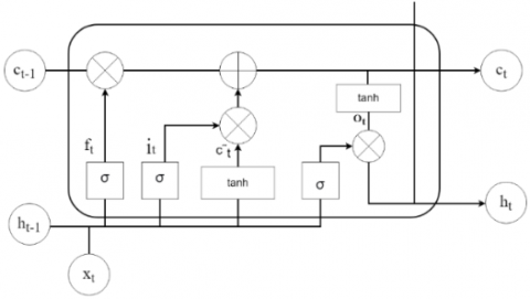
The Bidirectional Long Short-Term Memory (BiLSTM) model represents a significant improvement over the conventional LSTM architecture, LSTM the LSTM architecture is shown in Figure 1. This framework leverages the capability of two independent LSTMs operating simultaneously, one in the forward direction and the other in the backward direction. Over time, BiLSTM has established itself as a powerful machine learning technique, widely adopted across various research domains. One notable example is presented by Yu et al. [14] a Bi-directional Long Short-Term Memory (Bi-LSTM) framework was proposed to model movement uncertainty in crowdsourced human trajectories under complex urban environments. The model integrates GNSS data with pedestrian motion features such as gait length and heading deviation and demonstrates superior performance compared to baseline models including LSTM, MLP, and 1D-CNN. Experimental results show that the Bi-LSTM model achieves an average prediction error of just 1.82 meters and a coverage ratio of 98.1%, significantly outperforming traditional uncertainty modeling approaches like UB, AUB, and BAEE. This highlights Bi-LSTM’s robustness and adaptability in predicting spatial deviations caused by GNSS signal occlusion and urban complexity.in classification accuracy, recall, and F1-score.
Figure 1. LSTM architecture
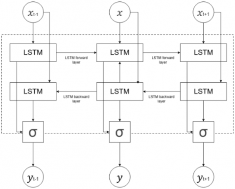
Figure 2. Bi-LSTM architecture
Structurally, Bi-LSTM employs two parallel stacks of LSTM layers that process the input sequence in opposite temporal directions, as illustrated in the Figure 2. The forward LSTM layer processes the sequence chronologically from earlier time steps h(t-1) to later ones (t+1), propagating information from the past. The backward LSTM layer processes the sequence in reverse, from future time steps (t+1) back to previous ones (t-1), capturing contextual information from the future. For any given time step t, the hidden state generated by the forward layer (representing past context) and the hidden state generated by the backward layer (representing future context) are combined typically by concatenation to form a comprehensive output vector. This integration of information from both temporal directions enables BiLSTM to capture richer contextual dependencies compared to traditional unidirectional LSTM models [13, 14].
2.3 Attention mechanism
The attention mechanism has become a central concept in deep learning, inspired by human cognitive processes that selectively focus on the most informative aspects of incoming data. By allowing neural networks to dynamically emphasize relevant features while suppressing less useful information, attention improves computational efficiency and enhances predictive accuracy across diverse tasks, including image captioning, speech recognition, and text classification. Over time, it has developed into various forms such as soft, hard, self-attention, and multi-head attention, and has been successfully integrated into architectures like RNNs and CNNs. Beyond improving performance, attention also contributes to interpretability, as the visualization of attention weights provides insights into the model’s decision-making process [15].
In parallel, the evolution of attention has further shaped modern deep learning, particularly with the emergence of the Transformer architecture. Unlike earlier models that relied on recurrence or convolution, Transformers rely solely on attention mechanisms, marking a significant paradigm shift in how sequence modelling is approached. Originating from biologically inspired ideas of selective focus, attention has matured into a flexible and powerful computational tool, enabling breakthroughs across domains such as neural machine translation and multimodal learning. As the field continues to advance, attention remains a foundational component for building adaptive, context-aware, and highly effective neural network systems [16].
Eq. (1) defines the context vector ct, which is derived as a weighted sum of the hidden representations hj. Here, $\alpha_{t j}$ corresponds to the attention coefficients that determine the relative importance of each hidden state with respect to the current time step. By assigning higher weights to more informative features and lower weights to less significant ones, the attention mechanism enables the model to selectively focus on the most relevant parts of the input sequence while constructing ct.
$c_t=\sum_{j=1}^t \alpha_{t j} h_j$ (1)
The architecture of the attention mechanism, as shown in Figure 3, shows how context vectors are generated by integrating information from multiple hidden states. At each decoding step t, the model computes alignment scores between the current hidden state ht and all encoder hidden states hi. These scores are then normalized using the softmax function to produce attention weights $\alpha_{t i}$, which indicate the relative contribution of each hidden state. The weighted sum of hidden states forms the context vector ct, which is combined with the decoder hidden state ht to generate the output yt. This process allows the decoder to adaptively focus on different parts of the input sequence depending on the current prediction step. In practice, this mechanism improves model ability to capture long-range dependencies, reduces information loss commonly found in fixed-length context representations, and enhances both accuracy and interpretability [16].
Figure 3. Attention mechanism
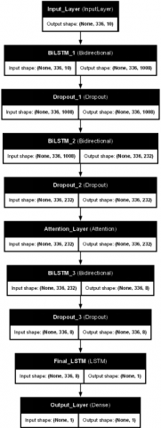
In the BiLSTM with Attention model, the process starts with a Bidirectional LSTM layer. This layer extracts information from both directions of the time sequence. Next, a Dropout layer reduces the risk of overfitting. A second Bidirectional LSTM deepens the representation of temporal features, and another Dropout layer follows it. Then, an Attention layer highlights important features in the data sequence. The results are processed by a third Bidirectional LSTM, which is also followed by Dropout to maintain learning stability. Finally, the output layer produces the final prediction value. The sequence of this architectural model is shown in the Figure 4.
Figure 4. Visualization of proposed BiLSTM with attention
2.4 Empirical Wavelet Decomposition
EWD is a frequency domain-based signal analysis method developed to adaptively decompose complex signals into several empirical modes based on their energy spectrum characteristics [16, 17]. Unlike the Discrete Wavelet Transform (DWT), which uses fixed basis functions such as Haar or Daubechies, EWD constructs wavelet filter banks empirically through signal spectrum segmentation. This approach makes EWD more flexible for analyzing nonlinear and nonstationary signals such as electricity loads affected by weather variations, consumption behavior, and seasonal patterns [2, 18].
The methodology involves three main steps. First, the signal’s spectrum is segmented into distinct regions, each corresponding to a unique mode of the signal. Next, an empirical wavelet filter bank is constructed to match the frequency content of each segment, ensuring perfect reconstruction of the signal. Finally, the signal is filtered through these wavelets, yielding a detailed time-frequency decomposition. Mathematically, f(t) represents the signal, EWD decomposes it into like writen in Eq. (2).
$f(t)=\sum_k W_k(t)+R(t)$ (2)
where, $W_k(t)$ are the wavelet coefficients, and $R(t)$ is the residual signal not captured by wavelet. The empirical wavelet are defined by Eq. (3), with $\psi k(t)$ representing the adaptive wavelet basis functions.
$W_k(t)=(f(t), \psi k(t))$ (3)
The empirical wavelet is based on the segmentation of the Fourier spectrum of a signal $f(t)$ into N distinct frequency bands. This segmentation is defined by a set of boundaries $\left\{\omega_i\right\} N_i=0$, where $\omega_0=0$ and $\omega_N=\pi$. For each segment, an empirical scaling function $\phi_n(\omega)$ and an empirical wavelet function $\psi n(\omega)$ are constructed. The empirical scaling function is defined as shown in Eq. (4).
$\phi_n(\omega)=\left\{\begin{array}{c}1, \omega \in\left[0, \omega_1\right] \\ \cos \left(\frac{\pi}{2} \frac{\omega-\omega_1}{\omega_2-\omega_1}\right), \omega \in\left(\omega_1, \omega_2\right] \\ 0, \text {otherwise}\end{array}\right.$ (4)
Similarly, the empirical wavelet functions is defined for n = 2, N as show in Eq. (5).
$\psi_n(\omega)=\left\{\begin{array}{c}\sin \left(\frac{\pi}{2} \frac{\omega-\omega_{n-1}}{\omega_n-\omega_{n-1}}\right), \omega \in\left(\omega_{n-1}, \omega_n\right) \\ \cos \left(\frac{\pi}{2} \frac{\omega-\omega_n}{\omega_{n+1}-\omega_n}\right), \omega \in\left(\omega_n, \omega_{n+1}\right) \\ 0, \text {otherwise}\end{array}\right.$ (5)
$f(t)=\sum_{n=1}^N\left(f_n\right)$ (6)
$f_n(t)=F^{-1}\left[\hat{f}(\omega) \cdot \psi_n(\omega)\right]$ (7)
Given functions 5 , the decomposes a signal $f(t)$ into $N$ components as follows in Eq. (6) where each component $f_n(t)$ is obtained by applying the inverse Fourier transform to the product of the signals Fourier transform and the respective filter is show in Eq. (7), where $f(t)$ is the original signal in the time domain, while $\widehat{f}(\omega)$ is the Fourier transform of that signal in the frequency domain. The function $\psi_n(\omega)$ acts as the n -th empirical wavelet or frequency filter that extracts signal components at a specific frequency band. The operation $F^{-1}$ meaning (inverse Fourier transform) then converts the result in the frequency domain back to the time domain, producing $f_n(t)$, the $n$-th empirical mode. Thus, each $f_n(t)$ represents a portion of the signal with specific frequency characteristics, and empirical modes can reconstruct the original signal [9, 19].
The research focuses on enhancing electricity load forecasting by combining weather data with a signal decomposition approach. The modelling framework is based on a Bi-LSTM with Attention, which is well-suited for capturing temporal dependencies while adaptively emphasizing the most influential patterns in the input. In the first stage, feature selection is carried out by evaluating correlation coefficients (CC) between weather variables and electricity load data, ensuring that only the most relevant weather features are retained. These selected features are then subjected to wavelet decomposition, enabling the extraction of both low- and high-frequency components that reflect long-term trends as well as short-term variations.
The decomposed weather signals, together with temporal indicators and electricity load data, are used as inputs for the Bi-LSTM with Attention model. The dataset is split into training and testing sets to evaluate the model’s predictive skill, while hyperparameter tuning is applied to further optimize its performance. By integrating pre-selection of weather variables with wavelet-based decomposition and an attention-augmented recurrent neural network, the proposed approach aims to achieve accurate and reliable electricity load forecasting.
3.1 Weather data
In this study, the input features for the machine learning model are derived from weather data provided by the European Center for Medium-Range Weather Forecasts (ECMWF) through the ERA5 reanalysis dataset [20], with an hourly temporal resolution. The selected region of interest is focused on the area surrounding Bali. The weather parameters considered as candidate features include temperature, solar radiation, wind speed, and pressure.
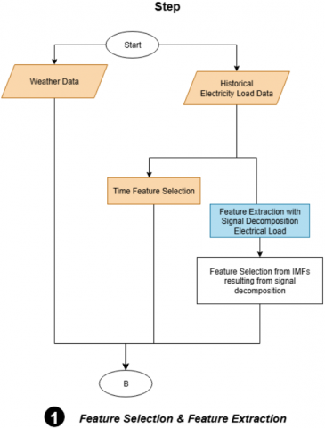
To explore the relationship between these weather variables and electricity load, scatter plot visualizations were employed alongside both linear and nonlinear regression analyses. Subsequently, the most relevant weather features for the machine learning model were identified by calculating their correlation coefficients (CC) with electricity load data. This process is summarized in the flowchart shown in Figure 5. This metric provides a quantitative measure of association, enabling the identification of weather parameters that exhibit the strongest influence on load variability.
Figure 5. Flowchart 1 - method to feture selection
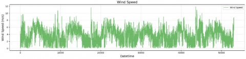
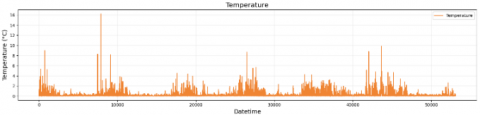
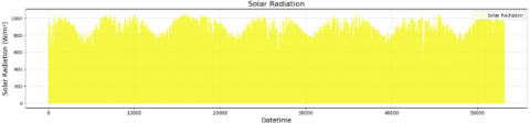
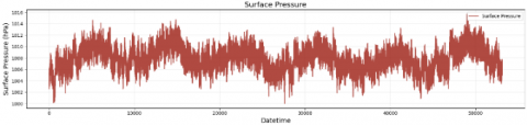
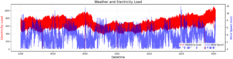
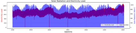
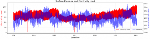
The weather dataset was obtained from the ERA5 reanalysis provided by ECMWF, covering the Bali region (8.25°S-8.75°S, 115°E-115.5°E) with an hourly temporal resolution from 1 January 2022 to 23 January 2024. The parameters include air temperature at 2 m (t2m), surface solar radiation (ssrd), wind speed (wnd), and surface pressure (spr). Figures 6-9 show the plot weather parameter. Missing or incomplete records (less than 1.5% of the total samples) were handled by linear interpolation to maintain temporal continuity. All weather variables were normalized using min–max scaling before being fed into the model.
Figure 6. Wind speed
Figure 7. Temperature
Figure 8. Solar radiation
Figure 9. Surface pressure
3.2 Electricity load data
This study concentrates on electricity load forecasting with a particular focus on the Bali region, which is characterized by its relatively isolated grid system and distinct electricity consumption patterns compared to larger interconnected areas. This study focuses on electricity load forecasting, with a particular focus on the Bali region, which is characterized by a relatively isolated electricity grid system and different electricity consumption patterns compared to more interconnected regions. Data were downloaded from the Global Forecast System (GFS) provided by NOAA, with weather prediction coverage up to 14 days in advance.
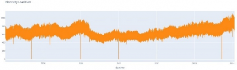
Figure 10. Electricity load data
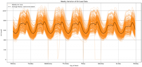
Figure 11. Electricity load data (weekly variation)
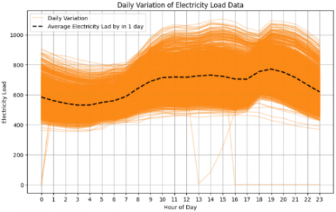
Figure 10 presents electricity load data over four years. Figure 11 displays Bali's average weekly electricity load data, while Figure 12 displays Bali's average daily electricity load data. The weekly power load data in Figure 11 indicate little variation in electricity consumption, though a decline is noted on weekends. In contrast, the daily electricity load data in Figure 12 indicate that the minimum average electricity consumption occurs around 2-4 o'clock, and the maximum average usage peaks at 19 o'clock.
Figure 12. Electricity load data (daily varitation)
The hourly electricity load data were collected from the PLN Research Institute for the same period as weather data (1 January 2022-23 January 2024) with target predict for 14 days (9-23 January 2024). The dataset represents the total regional demand in megawatts (MW) for the Bali power grid. Minor gaps in the load time series (< 0.5%) were filled using spline interpolation, while obvious outliers were replaced with the local mean of the previous and subsequent 3-hour windows.
3.3 Feature selection and extraction
First, the historical electricity load data are extracted and separated into load-related information and consumer behavior patterns. Next, feature selection is performed on the weather data obtained from the ERA5 reanalysis dataset. The candidate weather parameters include temperature, solar radiation, wind speed, and surface pressure. The selection process is based on the correlation coefficient between each weather parameter and the electricity load. In the subsequent step, the signals of the selected weather features are further decomposed using wavelet transformation to capture both short-term variations and long-term trends. Figure 13 illustrates the next stage following the analysis in Figure 12, where the selected features are integrated into the machine learning model to forecast electricity load.
Figure 13. Flowchart 2 - Input into machine learning
3.4 Selected feature
The selected features are further utilized to design a series of test scenarios aimed at evaluating the effectiveness of different inputs and methodological choices in improving the accuracy of electricity load forecasting. The test scenarios are organized as follows:
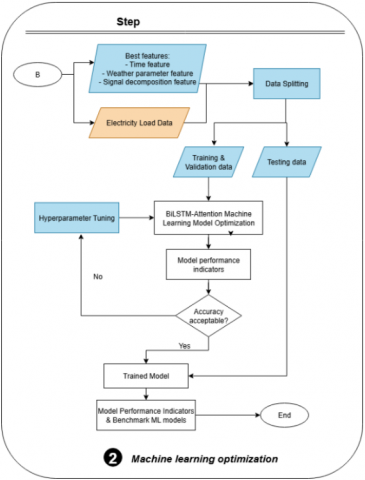
3.5 ML optimization
At this stage, the primary objective is to optimize the machine learning model in order to achieve accurate forecasting results. The prepared dataset is first divided into training and testing subsets. The model is then trained using the training data to capture underlying patterns and improve predictive accuracy. Once trained, the model is evaluated on the testing data, where its performance is measured using correlation coefficient (CC) [2], Root Mean Squared Error (RMSE) [3], and Mean Absolute Percentage Error (MAPE) [4]. In cases where the forecasting performance does not meet the desired standard, hyperparameter tuning is conducted through grid search to further enhance the model’s predictive capability. An overview of the training and testing data length is presented in Figure 14, while Table 1 summarizes the optimal layer configuration and corresponding model parameters.
Figure 14. Length data train and testing (electricity load)
The proposed Bi-LSTM-Attention model was optimized through grid search. The final configuration that yielded the best performance is summarized in Table 1. All baseline models (Bi-LSTM, XGBoost, AdaBoost, and MLP) were trained using identical training/testing splits and evaluation metrics to ensure a fair comparison.
Table 1. Result of correlation coefficient between
|
Parameter |
Description |
Value |
|
Input Shape |
Determine the number of time steps and the number of features. Inputs are adjusted based on the training dataset |
train_data.shape [1], train_data.shape [2] |
|
Activation |
Non-linear activation function that keeps the LSTM value stable |
tanh |
|
Recurrent Activation |
Used for input, output, and forget gates, regulating the temporal flow of information |
sigmoid |
|
BiLSTM First Layer |
A large-capacity primary layer for capturing long-term temporal patterns of data |
1008 |
|
BiLSTM Second Layer |
Feature filtering stage before entering the attention layer |
232 |
|
Attention Layer |
Assigns dynamic weights to each timestep based on its importance to the prediction output |
1 |
|
Dropout |
Additional regularization after attention to reduce over-reliance on a particular timestep |
0.1 |
|
BiLSTM Third Layer |
Layer that refines the attention results |
8 |
|
Epoch |
Maximum number of iterations |
10000 |
|
Batch size |
Provides a balance between weight update stability and memory efficiency |
32 |
|
Learning Rate |
Coefficients that control the learning rate of the model during the optimization process |
0.0005 |
|
Early Stopping |
The training process stops when the validation loss converges for 10 epochs, restoring the best weights to prevent overfitting and reduce training time |
Patience = 10 |
|
Loss Function |
A measure of how far the model's predictions are from the actual values |
MSE |
The aim in this research is to develop a weather-based power load forecasting system for Bali by integrating Empirical Wavelet Decomposition Bi-directional long short-term memory with attention mechanism. This section presents the results obtained from the proposed model under a variety of experimental scenarios designed to evaluate its forecasting performance. Each scenario has been carefully structured to highlight different aspects of the model’s capability, including the influence of weather parameters, the role of temporal features, the impact of wavelet-based signal decomposition, and the effect of training data length on predictive accuracy. By systematically analysing these scenarios, we aim to provide a comprehensive understanding of the model’s strengths and limitations when applied to electricity load forecasting in the Bali region.
The presentation of results is organized to facilitate a clear comparison across scenarios. First, we discuss the outcomes related to the selection of weather variables, identifying which parameters contribute most significantly to prediction accuracy. Next, we evaluate the role of temporal features such as hour of the day, day of the week, and seasonal indicators, which are expected to capture the cyclic behaviour of electricity consumption. We then examine the benefits of incorporating wavelet decomposition into the modelling pipeline, demonstrating how signal decomposition enhances the representation of weather data and improves forecasting precision. Finally, we assess how different lengths of training data influence the model’s generalization ability, offering insights into the trade-off between computational efficiency and predictive performance.
Through this structured approach, the reported results not only validate the effectiveness of the Bi-LSTM with Attention framework combined with wavelet decomposition but also provide a solid basis for discussing practical implications and potential areas for further improvement.
This research has 4 sensitivity test scenarios for each feature; the Table 2 contains the test scenarios in this research.
Table 2. Sensitivity test scenarios
|
1 |
Weather Parameter |
|
2 |
Time Feature |
|
3 |
Wavelet Decomposition |
|
4 |
Training Data Length |
4.1 Weather
Based on the results summarized in Tables 3 and 4, it is evident that the selection of input features has a substantial impact on the forecasting performance of the Bi-LSTM with Attention model. Table 3 presents the correlation coefficients between weather parameters and electricity load, while Table 4 compares the forecasting performance of different weather-based input configurations. When using temperature (t2m) alone as the input, the model achieved relatively poor performance, with a Correlation Coefficient (CC) of 0.44, Root Mean Square Error (RMSE) of 113.3 MW, and a Mean Absolute Percentage Error (MAPE) of 11.47%. This outcome indicates that temperature by itself is insufficient to fully capture the variability of electricity load.
Table 3. Result of correlation coefficient between weather and electricity load
|
Weather Parameter |
CC |
|
t2m |
-0.0877 |
|
ssrd |
0.4387 |
|
wnd |
0.1568 |
|
spr |
-0.0875 |
Table 4. Result of Bi-LSTM-Attention with various weather
|
Weather Input |
Performance |
||
|
CC |
RMSE (Mw) |
MAPE |
|
|
t2m |
0.44 |
113.3 |
11.47 |
|
t2m, ssrd |
0.93 |
45.58 |
4.18 |
|
t2m, ssrd, wnd |
0.93 |
55.5 |
5.27 |
|
t2m, ssrd, wnd, spr |
0.89 |
74.34 |
6.46 |
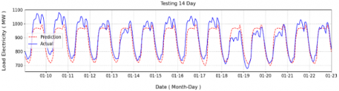
In contrast, the combination of temperature (t2m) and solar radiation (ssrd) provided the best results, with a CC of 0.93, a significantly reduced RMSE of 45.58 MW, and the lowest MAPE of 4.18%. This demonstrates that the inclusion of solar radiation as an additional feature greatly enhances the model’s predictive accuracy, making this input configuration the most effective among all tested scenarios.
Other combinations, such as t2m with ssrd and surface pressure (spr), maintained a high CC value of 0.93 but led to increased RMSE (55.5 MW) and MAPE (5.27%). Similarly, adding wind speed (wnd) alongside t2m, ssrd, and spr further degraded performance, with CC dropping to 0.89, RMSE rising to 74.34 MW, and MAPE increasing to 6.46%. These results suggest that including additional variables that are less strongly correlated with electricity load can negatively affect the model’s generalization ability. Figure 15 visualizes the actual and predicted electricity load using temperature and solar radiation as input features.
Figure 15. Actual and prediction with weather data (temperature and solar radiation)
Figures 16-19 illustrates the correlation between electricity load and wind speed. Therefore, the most effective configuration identified in this study is the Bi-LSTM with Attention model using temperature (t2m) and solar radiation (ssrd) as inputs, as this combination delivers the highest accuracy, lowest prediction error, and overall best balance across all performance metrics. the combination of temperature (t2m) and solar radiation (ssrd) yielded the best performance, with a CC of 0.93, RMSE of 45.58 MW, and the lowest MAPE of 4.18%.
Figure 16. Electricity load and wind speed
Figure 17. Electricity load and temperature
Figure 18. Electricity load and solar radiation
Figure 19. Electricity load and pressure
4.2 Time feature
The results, presented in Table 5, highlight clear differences in model performance across these feature sets. When weather data were combined with the hour feature, the model achieved particularly strong results, with a Correlation Coefficient (CC) of 0.93, RMSE of 46.45 MW, and the lowest Mean Absolute Percentage Error (MAPE) of 3.71%. This indicates that electricity load in the study region is highly sensitive to intra-day variations, and that the hour feature enables the model to capture these fluctuations effectively. When the day feature was added alongside weather and hour, however, performance slightly decreased, with CC dropping to 0.92, RMSE rising to 55.83 MW, and MAPE increasing to 5.02%. This suggests that day of the month alone provides limited information for capturing short-term demand variations.
Table 5. Result of Bi-LSTM-Attention with various time feature
|
Time Input |
Performance |
||
|
CC |
RMSE (Mw) |
MAPE |
|
|
Hour |
0.93 |
46.45 |
3.71 |
|
Hour, day |
0.92 |
55.83 |
5.02 |
|
Hour, day, DoW |
0.93 |
46.14 |
4.2 |
|
Hour, day, DoW, Month |
0.94 |
46.26 |
4.27 |
The inclusion of the day of the week (dow) feature together with weather and hour improved stability compared to the day-only configuration, yielding CC of 0.93, RMSE of 46.14 MW, and MAPE of 4.20%. This outcome reflects the influence of weekly consumption cycles, which can enhance prediction accuracy to a certain extent. Finally, extending the input feature set by adding month information produced the highest CC value of 0.94, but with slightly increased RMSE (46.26 MW) and MAPE (4.27%) relative to the hour-only setup. Although this suggests that monthly patterns contribute to capturing broader seasonal trends, the results confirm that their predictive value is secondary compared to the dominant effect of hourly variations.
Taken together, these findings demonstrate that the hour feature is the most influential temporal variable when combined with weather data, as it delivers the most accurate and reliable forecasts with the lowest MAPE. While additional temporal indicators such as day, dow, and month can marginally improve correlation, they introduce higher errors that reduce practical forecasting accuracy. Therefore, the combination of weather and hour was selected as the most optimal input configuration, as it strikes the best balance between strong correlation (CC = 0.93) and forecasting accuracy (MAPE = 3.71%).
4.3 Wavelet decomposition results
To further refine the model performance, signal decomposition using wavelet-based was applied to the selected weather features, specifically temperature (t2m) and solar radiation (ssrd), which had previously been identified as the most effective variables when combined with the hour feature. The purpose of this decomposition was to reduce high-frequency fluctuations and noise in the input data, thereby enabling the model to better capture the underlying trends of electricity consumption. In this process, only the approximation component (A) of the decomposed signal was retained, while the high-frequency detail component (H) was discarded, as it was considered less informative for load forecasting.
Table 6. Result of Bi-LSTM-Attention
|
Input |
Performance |
||
|
CC |
RMSE (Mw) |
MAPE |
|
|
Normal Input |
0.93 |
46.45 |
3.71 |
|
Wavelet Input |
0.93 |
42.58 |
3.92 |
The results of this experiment, as summarized in Table 6, show that the integration of wavelet decomposition with weather data produced notable improvements in model performance. Specifically, the Bi-LSTM with Attention model using the normal input achieved a Correlation Coefficient (CC) of 0.93, RMSE of 46.45 MW, and MAPE of 3.71%. When the weather features were pre-processed with wavelet decomposition, the CC value remained unchanged at 0.93, but the RMSE improved to 42.58 MW, demonstrating a reduction in prediction error. However, the MAPE slightly increased to 3.92%, indicating a minor trade-off in percentage-based accuracy. Figure 20 presents the prediction results obtained using wavelet decomposed features, while Figure 21 shows the prediction results without applying wavelet decomposition. The comparison between these two figures demonstrates that incorporating wavelet decomposition leads to smoother forecasting results, effectively reducing short-term fluctuations and noise in the predicted electricity load.
Figure 20. Prediction results with wavelet
Figure 21. Prediction result without wavelet
Overall, these findings confirm that wavelet decomposition contributes positively to stabilizing and smoothing the input signals, particularly by reducing noise-related variations that could mislead the learning process. Although the improvement is more apparent in RMSE rather than MAPE, this step further enhances the robustness of the forecasting framework, ensuring more consistent predictions under fluctuating weather conditions.
4.4 Training data length
Following the integration of wavelet decomposition into the weather inputs, further experiments were conducted to evaluate the impact of training data length on forecasting performance. The Bi-LSTM with Attention model was trained using three different training windows 3 months, 6 months, and 12 months.
Table 7. Result of Bi-LSTM-Attention with various length
|
Data Length |
Performance |
||
|
CC |
RMSE (Mw) |
MAPE |
|
|
3 Months |
0.93 |
42.58 |
3.92 |
|
6 Months |
0.95 |
32.75 |
2.7 |
|
12 Months |
0.94 |
50.4 |
4.38 |
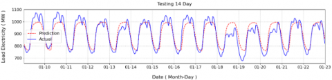
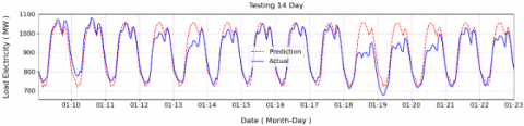
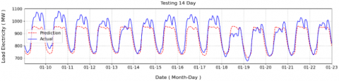
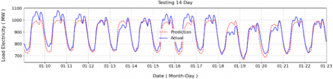
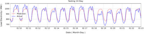
The results, presented in Table 7, show that the training length significantly influences the accuracy and robustness of the forecasting model. With a 3-month training dataset, the model achieved a Correlation Coefficient (CC) of 0.93, RMSE of 42.58 MW, and MAPE of 3.92%. Extending the training length to 12 months, however, did not yield better results, as performance declined slightly with CC of 0.94, RMSE of 50.4 MW, and MAPE of 4.38%. Interestingly, the optimal configuration was obtained when the model was trained on 6 months of data, producing the best forecasting outcomes with CC of 0.95, RMSE of 37.48 MW, and MAPE of 3.26%. Figures 22-24 illustrate the visual differences in prediction performance across various training data lengths. Figure 22 shows the results for a 12-month training period, Figure 23 presents the outcomes for 6 months of training, and Figure 24 displays the predictions based on 3 months of training data. These visual comparisons highlight that the 6-month training window show stable and forecasts.
Figure 22. Prediction results with length 12 months
Figure 23. Prediction results with length 6 months
Figure 24. Prediction results with length 3 months
These findings suggest that providing the model with too little historical data limits its ability to learn complex load–weather interactions, while excessively long training windows may introduce outdated or less relevant patterns that reduce generalization performance. The 6-month window offered the best balance between capturing sufficient variability in the input features and avoiding overfitting to long-term seasonal fluctuations.
Overall, this analysis highlights the importance of selecting an appropriate training length in electricity load forecasting. By combining wavelet decomposition with a 6-month training dataset, the Bi-LSTM with Attention model achieved its best predictive accuracy, reinforcing the effectiveness of the proposed framework for STLF.
4.5 Model comparison
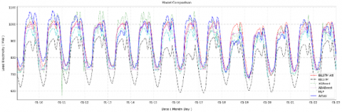
The final stage of the evaluation involved comparing the proposed Bi-LSTM with Attention model incorporating wavelet decomposition against several benchmark models, including Bi-LSTM, XGBoost, AdaBoost, and MLP, all tested with normal input configurations. The performance results are presented in Table 8, which compares the proposed Bi-LSTM with Attention model incorporating wavelet decomposition against several benchmark models. Figure 25 provides a visual comparison of all models, clearly illustrating the performance differences across the Bi-LSTM, Bi-LSTM with Attention, XGBoost, AdaBoost, and MLP models.
Table 8. Result of Bi-LSTM-Attention with various model
|
Model |
Performance |
||
|
CC |
RMSE (Mw) |
MAPE |
|
|
Bi-LSTM-Att |
0.95 |
32.75 |
2.7 |
|
Bi-LSTM |
0.93 |
120.82 |
12.66 |
|
XGBoost |
0.94 |
42.59 |
3.55 |
|
AdaBoost |
0.94 |
43.2 |
3.96 |
|
MLP |
0.92 |
61.86 |
5.37 |
Figure 25. Model comparison
Specifically, the Bi-LSTM with Attention using wavelet decomposition achieved the highest performance across all metrics, with a Correlation Coefficient (CC) of 0.95, RMSE of 37.48 MW, and MAPE of 3.26%. These results represent a significant improvement compared to the same architecture without wavelet decomposition, where CC was 0.94, RMSE increased to 56.76 MW, and MAPE rose to 5.38%. Similarly, while tree-based models such as XGBoost and AdaBoost demonstrated competitive results, with RMSE values of 42.59 MW and 43.2 MW respectively, and MAPE values of 3.55% and 3.96%, they still fell short of the proposed method in terms of both accuracy and robustness. The MLP model performed the weakest overall, with a CC of 0.92, RMSE of 61.86 MW, and MAPE of 5.37%.
To ensure that the forecasting accuracy is statistically proven, a t-test was performed on BiLSTM without attention and BiLSTM with attention based on the RMSE value. The results show a t-statistic of 276.48 and a p-value of 1.03 × 10⁻⁹, which is far below the threshold of 0.05, indicating that BiLSTM-Attention exhibits a statistically significant improvement. Furthermore, the 95% confidence interval for the RMSE difference between 87.41 MW and 89.19 MW indicates a consistent and substantial decrease in forecasting error.
These findings confirm that the integration of wavelet decomposition with Bi-LSTM and Attention not only enhances the model’s capability in handling high-frequency noise in weather data but also establishes it as the most effective approach among the tested models. By leveraging the combined strengths of temporal feature extraction, attention mechanisms, and signal decomposition, the proposed framework delivers the most accurate and reliable electricity load forecasting results in the study.
This study proposed an electricity load forecasting framework utilizing a Bi-LSTM with Attention model combined with wavelet decomposition to improve prediction accuracy by effectively filtering high-frequency noise from weather signals. The evaluation process was systematically conducted through several stages, beginning with the identification of the most relevant weather parameters, the incorporation of temporal features, the application of wavelet-based signal decomposition, and finally a comparative analysis against other machine learning models.
The results indicate that the optimal feature configuration consists of temperature (t2m) and solar radiation (ssrd) combined with hourly information and six months training data length, which effectively captures intra-day consumption cycles that strongly influence electricity demand in the study area. Furthermore, applying wavelet decomposition to weather signals significantly enhanced the forecasting performance. The proposed Bi-LSTM with Attention model with wavelet decomposition achieved the best overall results, with a Correlation Coefficient (CC) of 0.95, Root Mean Square Error (RMSE) of 32.75 MW, and Mean Absolute Percentage Error (MAPE) of 2.7%. These values surpass the performance of other benchmark models, including Bi-LSTM, XGBoost, AdaBoost, and MLP, thereby confirming the superiority of the proposed approach in terms of both accuracy and reliability.
In summary, this research demonstrates that integrating deep learning architectures with signal decomposition techniques offers a highly effective solution for electricity load forecasting, particularly in regions where demand is sensitive to both weather and temporal variations. Nonetheless, the study is limited by the scope of input features and geographical coverage. Future research can be developed by extend the dataset with broader temporal and spatial coverage, incorporate additional influencing factors such as socioeconomic or demographic variables, while also considering new factors such as tourist crowds that influence electricity consumption patterns in tourist areas. Additionally, including weather variables such as rainfall and humidity can offer a more comprehensive representation of meteorological conditions. Exploring advanced hybrid or ensemble learning approaches is expected to improve the accuracy and robustness of forecasting systems in dynamic electricity systems.
This research was funded by Kementerian Pendidikan, Kebudayaan, Riset dan Teknologi, Republik Indonesia, research grant numbers 125/C3/DT.05.00/PL/2025 and 060/LIT07/PPM-LIT/2025.
|
t2m |
Tempature at 2 meters (°C) |
|
ssrd |
Solar Radiation W/m2 |
|
wnd |
m/s |
|
Spr |
Surface Pressure |
|
hour |
Time indicator electricity load |
|
day |
Time indicator electricity load |
|
DoW |
Day of Week (time indicator electricity load) |
|
month |
Time indicator electricity load |
|
CC |
Correlation Coefficient |
|
RMSE |
Root Mean Square Error |
|
MAPE |
Mean Absolute Percentage Error |
|
X low |
Approximation Components |
|
X high |
Detail Components |
|
hj |
Hidden state of j-th time step |
|
Ct |
Context vector in attention mechanism |
|
$\mathrm{W} \psi$ |
Wavelet transform coefficient |
|
ht+1 |
Forward step |
|
ht-1 |
Backward step |
|
Greek symbols |
|
|
atj |
Attention weight coefficient |
|
$\psi$ |
Mother wavelet function |
|
Subscripts |
|
|
dk |
Coefficient low pass filter in wavelet |
|
t |
Time step index |
|
j |
Hidden state index |
|
ck |
Coefficient high pass filter in wavelet |
[1] Wang, J., Azam, W. (2023). Natural resource scarcity, fossil fuel energy consumption, and total greenhouse gas emissions in top emitting countries. Geoscience Frontiers, 15(2): 101757. https://doi.org/10.1016/j.gsf.2023.101757
[2] Aditya, I.A., Adytia, D. (2025). Modelling of spatially correlated weather-based electricity forecasting using combined frequency-based signal decomposition with optimized boosting approach. International Journal of Electrical Power and Energy Systems, 169: 110698. https://doi.org/10.1016/j.ijepes.2025.110698
[3] Nepal, B., Yamaha, M., Yokoe, A., Yamaji, T. (2019). Electricity load forecasting using clustering and ARIMA model for energy management in buildings. Japan Architectural Review, 3(1): 62-76. https://doi.org/10.1002/2475-8876.12135
[4] Chodakowska, E., Nazarko, J., Nazarko, Ł. (2021). ARIMA models in electrical load forecasting and their robustness to noise. Energies, 14(23): 7952. https://doi.org/10.3390/en14237952
[5] Yin, C., Liu, K., Zhang, Q., Hu, K., Yang, Z., Yang, L., Zhao, N. (2023). SARIMA-based medium- and long-term load forecasting. Strategic Planning for Energy and the Environment, 42(2): 283-306. https://doi.org/10.13052/spee1048-5236.4222
[6] Bilgili, M., Pinar, E. (2023). Gross electricity consumption forecasting using LSTM and SARIMA approaches: A case study of Türkiye. Energy, 284: 128575. https://doi.org/10.1016/j.energy.2023.128575
[7] Xu, H., Hu, F., Liang, X., Zhao, G., Abugunmi, M. (2024). A framework for electricity load forecasting based on attention mechanism time series depthwise separable convolutional neural network. Energy, 299: 131258. https://doi.org/10.1016/j.energy.2024.131258
[8] Sekhar, C., Dahiya, R. (2023). Robust framework based on hybrid deep learning approach for short term load forecasting of building electricity demand. Energy, 268: 126660. https://doi.org/10.1016/j.energy.2023.126660
[9] Fan, G.F., Zheng, Y., Gao, W.J., Peng, L.L., Yeh, Y.H., Hong, W.C. (2023). Forecasting residential electricity consumption using the novel hybrid model. Energy and Buildings, 290: 113085-113085. https://doi.org/10.1016/j.enbuild.2023.113085
[10] Nabavi, S.A., Mohammadi, S., Motlagh, N.H., Tarkoma, S., Geyer, P. (2024). Deep learning modeling in electricity load forecasting: Improved accuracy by combining DWT and LSTM. Energy Reports, 12: 2873-2900. https://doi.org/10.1016/j.egyr.2024.08.070
[11] Park, J., Hwang, E. (2021). A two-stage multistep-ahead electricity load forecasting scheme based on LightGBM and Attention-BiLSTM. Sensors, 21(22): 7697. https://doi.org/10.3390/s21227697
[12] Wang, D., Li, S., Fu, X. (2024). Short-term power load forecasting based on secondary cleaning and CNN-BILSTM-attention. Energies, 17(16): 4142-4142. https://doi.org/10.3390/en17164142
[13] Graves, A., Schmidhuber, J. (2005). Framewise phoneme classification with bidirectional LSTM and other neural network architectures. Neural Networks, 18(5-6): 602-610. https://doi.org/10.1016/j.neunet.2005.06.042
[14] Yu, Y., Yao, Y., Liu, Z., An, Z., Chen, B., Chen, L., Chen, R. (2023). A Bi-LSTM approach for modelling movement uncertainty of crowdsourced human trajectories under complex urban environments. International Journal of Applied Earth Observation and Geoinformation, 122: 103412. https://doi.org/10.1016/j.jag.2023.103412
[15] Adytia, D., Latifah, A.L., Saepudin, D., Tarwidi, D., Pudjaprasetya, S.R., Husrin, S., Sopaheluwakan, A., Prasetya, G. (2024). A deep learning approach for wind downscaling using spatially correlated global wind data. International Journal of Data Science and Analytics, 20(3): 2721-2735. https://doi.org/10.1007/s41060-024-00629-3
[16] Niu, Z., Zhong, G., Yu, H. (2021). A review on the attention mechanism of deep learning. Neurocomputing, 452: 48-62. https://doi.org/10.1016/j.neucom.2021.03.091
[17] Soydaner, D. (2022). Attention mechanism in neural networks: Where it comes and where it goes. Neural Computing and Applications, 34(16): 13371-13385. https://doi.org/10.1007/s00521-022-07366-3
[18] Sithara, S., Pramada, S.K., Thampi, S.G. (2020). Sea level prediction using climatic variables: A comparative study of SVM and hybrid wavelet SVM approaches. Acta Geophysica, 68(6): 1779-1790. https://doi.org/10.1007/s11600-020-00484-3
[19] Zhang, D. (2019). Wavelet Transform. Texts in Computer Science, pp. 35-44. https://doi.org/10.1007/978-3-030-17989-2_3
[20] Hersbach, H., Bell, B., Berrisford, P., Hirahara, S., et al. (2020). The ERA5 global reanalysis. Quarterly Journal of the Royal Meteorological Society, 146(730): 1999-2049. https://doi.org/10.1002/qj.3803