Zahraa S. Kareem*![]() | Gregor A. Aramice
| Gregor A. Aramice![]() | Abbas H. Miry
| Abbas H. Miry ![]()
© 2025 The authors. This article is published by IIETA and is licensed under the CC BY 4.0 license (http://creativecommons.org/licenses/by/4.0/).
OPEN ACCESS
The position of the sensor node stands as a pivotal challenge in WSN applications. The efficacy of wireless communication systems is markedly limited by the attributes of the wireless channel, thereby amplifying the necessity for predicting channel path loss. Consequently, we undertook an empirical assessment of signal strength and path loss in relation to over which the link between Tx and Rx remains uninterrupted while maintaining acceptable path loss. Through the execution of an experiment in outdoor settings to evaluate the distance between nodes. The assessment utilized the LNSM algorithm, which relied on the RSSI values collected by the (transmitting) node’s receiving unit. Additionally, factors of the propagation channel, including standard deviation and path loss exponent values, were scrutinized. RSSI values for outdoor environment were recorded and examined for distances spanning from 1 to 90 m. The analysis disclosed an MAE error of 2.03 m and 1.80 m for ranges of 0-65 m and 0-100 m, respectively, alongside an RMSE error of 10 m and 8.71 m for the same distances associated with Zigbee. In contrast, Wi-Fi technology exhibited lower error rates across all distance measurements compared to Zigbee, underscoring its efficacy and dependability even over extended ranges. The MAE error stood at 0.33 m and 0.94 m for distances of (0-65 m) and (0-100 m), respectively, while the RMSE error was measured at 1.34 m and 5.31 m for the same distances. These findings indicate that LNSM is optimal for short distances when using Zigbee, whereas it can be used for longer distances when using Wi-Fi.
log normal shadowing model, Received Signal Strength Indicator, path loss exponent, wireless sensor networks, standard deviation, Mean Absolute Error, Root Mean Square Error
Wireless Sensor Networks (WSNs) consist of many elements that collaborate to monitor and gather data on multiple surroundings. They are usually termed as sensing elements, communication modules, processing units and energy supplies; where each part is critical for WSNs to operate complexly to perform functions such as data acquisition, data processing, data transfer, etc., which are significant for applications ranging from environment monitoring to structural integrity monitoring.
It is conceivable that an array of base stations and/or actuators may also be employed in WSNs. A significant portion of the scholarly endeavors surrounding WSNs (such as routing, medium access control, position estimation, synchronization, lifetime optimization, modulation, error correction, and security) are inherently tied to the transmission media and precise propagation models of signals among sensor nodes. The fidelity and exactness of the utilized propagation model play a crucial role in determining the coverage area, the chosen transmission power, and the longevity of the network. A faithful reconstruction of WSN topologies can be achieved if the path-loss metrics among the sensor nodes are derived using suitable propagation models [1]. These models are designed to incorporate the true-mode propagation characteristics of the electromagnetic waves that are used to convey information in a conventional simplified form (i.e., a model with a minimum number of parameters). It is essential for the design and assessment of WSN systems that proper modeling of propagation and path loss is performed [2].
Having a suitable path loss model, we can predict the attenuation of signals passing through a radio frequency channel. mmWave short wavelengths are subjected to significant signal attenuation due to mechanisms like reflection, scattering, line-of-sight (LOS) propagation, diffraction, and material penetration. Over the last few years, a wide variety of scenarios to replicate different measurements and models have been presented by several companies and research institutes [3].
While signals traversing their environment are subject to attenuation from barriers, distance, interference, and the nature of the physical components of the medium itself. Path loss leads to weaker signals, which might cause communication failures, low signal quality, and increased noise sensitivity. This forces nodes to use high transmission power to create reliable communication links. Nevertheless, operation at these higher power levels is costlier in terms of the energy requirements, which reduces the battery life at each node, thus compromising the lifetime of the whole network. As a result, path loss is directly related to link quality, energy efficiency, and therefore, the lifetime of the network. Introduction WSNs are an emerging networking technology that can provide reliable and efficient wireless communication by precise modeling of path loss and mitigation strategy [4].
Generally, WSN consists of five basic layers of its framework, including physical, data link, network, transport, and application layers [5]. But research [6] emphasizes the essential role of a physical layer in signal propagation dynamics to detect signals, the modulator, power allocation, frequency choice, and signal generation.
The Received Signal Strength Indicator (RSSI) can combine with the applied path loss and the shadowing models to obtain the Euclidean distance between nodes inside the network [7]. RSSI is a less expensive technique because it does not need (1) extra hardware (2) synchronization of time (3) a complicated antenna arrangement, but it is also not accurate. This approach is commonly used in WSNs to determine the locations of nodes in the network based on distance measurements [8].
In this study, the RSSI method will be used to find out where a contract is located. Since RSSI values are significantly affected by the conditions of the communication channel, so we are using a path loss model to calculate the distance between the mobile and the stationary nodes of a wireless Wi-Fi and Zigbee network based on RSSI data Log-Normal Shadowing Model (LNSM).
In this study, we focused on the LNSM because it is commonly used to model the wireless channel path loss for the fixed range between transmitter and receiver or to locate the node in outdoor environments.
1.1 Problem deviation
The main problem in WSN networks is that nodes are scattered randomly without any thought. This careless setup could make the signal less strong or less connected.
1.2 Objective
The study suggests using the LNSM framework to measure node separation with RSSI readings. This will make sure that the enhanced signal quality and data flow have minimal degradation. This makes wireless communication networks faster, more reliable, and more useful.
1.3 Impact of this manuscript
• Setting the physical path loss parameters, like path loss exponents and standard deviation.
• Use the path loss model based on outside conditions to figure out how far apart transmitters (Tx) and receivers (Rx) are.
• Find out how the height of the antenna affects how well it receives signals.
Zheng et al. [9] examined the implementation challenges of node localization in wireless sensor networks, tackled the challenges of environmental factors on RSSI readings, and presented solutions to enhance accuracy through tuning of model parameters. To improve precision, they are explaining how the measurement model parameters are identifiable with anchor nodes (otherwise called beacon nodes). These results suggest that this improved method can achieve better localization results that are essential for wireless sensor networks. Chen et al. [10] the propagation of Zigbee signals in a heavy electromagnetic noise environment in a substation was tested. We had a lot of testing to determine how Zigbee signals behave in these scenarios. Zigbee network Ground wire real-time monitoring system It promotes ease of monitoring of ground wire — a safety necessity in electrical works. It involves testing the path loss of ZigBee wireless signals in a highly electromagnetic interference substation environment. Signal within those conditions is weakened and suffers in reliability, so that makes it even more important.
An example of outdoor distance estimation. Has been developed by Latif Mohammed [8] effectively utilized the RSSI measurements to determine the distance from a Zigbee mobile node to a Zigbee coordinator node. This method really emphasizes that RSSI can be used as a distance approximation in the real world. The research was about the design of an LNSM designed for outdoor applications. It examined basic attributes of channels like standard deviation and path loss exponent, which are crucial for accurate signal propagation modeling. We used some metrics (such as correlation coefficient, Mean Absolute Error (MAE), and Root Mean Square Error (RMSE)) to evaluate the accuracy of distance estimation against the ground truth. Wu et al. [11] utilize different methods to investigate the transmission of radio frequency (RF) signals. The RSSI and the Packet Loss Rate (PLR) This is justified by the results, where the RSSI decreases while the PLR increases with a higher distance between the transmitter and receiver node. This indicates that the path loss decreases with increasing antenna height. To determine which model best fit the collected data, the researchers evaluated parametric exponential decay (OFPED) models as well as linear logarithmic models.
Benkič et al. [12] examine RSSI and Link Quality Indicator (LQI) metric in Zigbee-based wireless networks. These metrics are essential for assessing network node communication link quality. For wireless network analysis, the authors used the ZENA module on the CC2420 chip. This USB-connected module received packets on a designated channel and sent them to a PC for analysis. The ZENA software's user interface displayed captured packets, allowing researchers to examine their experiment data. In WSNs, many autonomous sensors are randomly distributed over an area, according to Supreeth and Akhil [13]. RSSI measurements are needed to locate the node. A comprehensive trilateration approach is presented to address WSN localization issues. The accuracy and reliability of Angle of Arrival (AoA) and Residual Analysis in trilateration validation were evaluated. These methods performed differently, with residual analysis performing best.
3.1 Communication technologies
3.1.1 Zigbee
Zigbee technology, which is predicated on the IEEE 802.15.4 standard, traverses multiple radio frequency bands, including 2.4 GHz, 915 MHz, and 868 MHz, and attains an exceptional data transmission rate of 250 kbps. Notably, Zigbee possesses the capability to function in a low-power sleep mode, facilitating prolonged battery life [14]. The system encompasses a variety of networking methodologies, integrating star, tree, and mesh configurations, which culminate in three principal categories of Zigbee networks: star, tree, and wireless mesh network architectures [15].
3.1.2 Wi-Fi
A wireless local area network (WLAN) is crafted in alignment with the IEEE 802.11 framework [16]. As the digital landscape evolves, Wi-Fi has risen to prominence across numerous sectors. It offers impressive communication speeds, robust signal coverage, rapid data exchange, and substantial bandwidth. Nonetheless, this technology heavily relies on bandwidth, and signal disruptions can lead to operational hiccups [17]. Wi-Fi's security features leave much to be desired, making it vulnerable to breaches and data losses in agricultural surveillance. Moreover, Wi-Fi struggles to handle significant amounts of agricultural information. Its networking capacity is limited, typically supporting only a handful of devices, often in the dozens, making it ill-suited for large-scale irrigation networks [17]. This technological innovation spans a wide array of radio frequencies, ranging from 2.4 to 60 GHz, while precisely outlining the structure of data packets. Wi-Fi has gained remarkable traction across various devices, largely due to its impressive operational range, usually between 3 and 7 km, aided by a high-efficiency transmitting antenna, along with its capability to achieve data transfer speeds that can soar up to 700 Mbps [14].
3.2 Processing unit
3.2.1 Arduino Uno R4 Wi-Fi
The Arduino® UNO R4 Wi-Fi is the first UNO board to feature a 32-bit microcontroller and an ESP32-S3 Wi-Fi® module (ESP32-S3-MINI-1-N8). It features an RA4M1 series microcontroller from Renesas (R7FA4M1AB3CFM#AA0), based on a 48 MHz Arm® Cortex®-M4 microprocessor. The UNO R4 Wi-Fi's memory is larger than its predecessors, with 256 kB flash, 32 kB SRAM, and 8 kB of EEPROM. The RA4M1's operating voltage is fixed at 5 V, whereas the ESP32-S3 module is 3.3 V. Communication between these two MCUs is performed via a logic level translator (TXB0108DQSR).
3.2.2 Raspberry Pi
An economical, sleek, Linux-driven circuit board, adept at connecting with a monitor and keyboard/mouse, offers a cost-effective means to interact with electronic systems while also acting as a foundation for coding or even enabling basic web services. It is crucial to highlight that this gadget does not support analog input like the Arduino, thereby requiring the use of an external Analog -to- Digital Converter (ADC) or an interfacing board to accomplish such tasks. MySQL can be incorporated within the board, allowing a General-Purpose Input/Output (GPIO) pin to serve as either a digital input or output, both functioning at a voltage level of 3.3V [18].
3.3 Wireless channel model based LNSM
Radio wave propagation happens when the wireless signal transmits in the air. The power of the transmitted signal will be attenuated by several parameters such as reflection, deflection, scattering, shadowing, and diffraction, which are the primary mechanisms that affect the propagation on the wireless channel [19]. Most wireless channel models are derived on the basis of a combination of analytical and practical methods [20]. The practical method has an advantage of taking into account all propagation parameters in the channel [20].
The efficacy of localization is intricately connected to the radio propagation model employed, with one such model being utilized in our computational simulation for the analysis of RSSI values. To delineate radio propagation, one of these models is [21].
Path-loss normal shadowing model: This model illustrates the correlation between distance and received power, as indicated by RSSI, through Eq. (1) [22]:
$P_r(d)=P_t-P_L\left(d_0\right)-10 \beta \cdot log _{10}\left(\frac{d}{d_0}\right)+X_\sigma$ (1)
The relationship between distance and path loss can also be shown by the following Eq. (2) [21]:
$P_L(d)=P_L\left(d_0\right)+10 \beta log _{10}\left(\frac{d}{d_0}\right)+X_\sigma$ (2)
Thus, from the equations above, Eq. (3) can be inferred [21]:
$P_r(d)=P_t-P_L(d)$ (3)
Yet, given that the log-distance path loss model reveals a logarithmic decline in the received power as the distance ($d$) grows, the mean received power at distance ($d$), represented as ($\operatorname{Pr}(d)$)), can be articulated as shown in Eq. (4) [23].
$P_r(d)=P_r\left(d_0\right)-10 \beta log _{10}\left(\frac{d}{d_0}\right)$ (4)
where,
$\mathrm{P}_{\mathrm{r}}(\mathrm{d})$: Received power in a specific distance d in dBm is essentially the same RSSI Consequently, we can derive the expression presented in Eq. (5) [23].
$R S S I(d)=R S S I\left(d_0\right)-10 \beta log _{10}\left(\frac{d}{d_0}\right)+X_\sigma$ (5)
The standard deviation (σ) between the observed and the computed RSSI sample locations provides an effective gauge for the shadow fading characteristic. (σ) is articulated as shown in Eq. (6) [23].
$\sigma=\frac{\sqrt{\sum_1^N({ measured }\ R S S I-{ calculated }\ R S S I)^2}}{N}$ (6)
where,
$P_t$: Transmitted power in dBm;
$P_L\left(d_0\right)$: Is the path loss for the specific distance $d_0$;
$\beta$: path loss exponent;
$X_\sigma$: is random shadowing effect ($X_\sigma$ ~ N (0, σ2)) with standard; deviation ($\sigma$) and with zero mean and σ2 variance;
$X_\sigma$equals zero without attenuation;
$P_L(d)$: Is the path loss for the specific distance $d$ in decibels.
4.1 Configuration of Zigbee
The components of Zigbee underwent a rebranding. The transmitting Zigbee unit became known as the coordinator, while the receiving unit was designated the End Device. Additionally, the API mode was initiated to facilitate the transmission and reception of packets.
In Application Programming Interface (API) mode, various packets of information are intricately woven into an API frame. This frame facilitates both the sending and receiving of data via wireless communication. Additional details incorporated into the API frame include a start delimiter, checksum, and the origins and destinations of the data. The start delimiter serves as the initial byte of the frame, signalling the commencement of the frame for easier detection and separation of frames. The length indicates the total byte count within the data frame. The data frame encompasses the data along with the source MAC address. The checksum, found as the final byte in the frame, is utilized to identify any errors that may arise during transmission and reception.
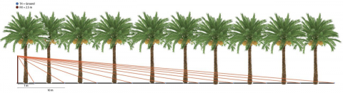
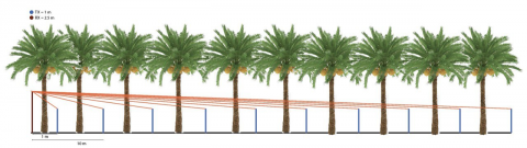
4.2 Evaluation of signal strength and path loss model
We undertook a comprehensive experimental evaluation of signal strength and path losses in relation to the communication technologies Zigbee and Wi-Fi, subsequently determining the greatest distance over which the connection endures uninterrupted between the Tx and Rx under acceptable path loss conditions; this assessment was conducted across varying distances (10m-90m) and transmitter heights (ground, 0.5m, 1m), while the receiver height was consistently maintained at 2.5m. The analysis involved Zigbee technology, utilizing a PC as the transmitter via the X-CTU program and an Arduino Uno R4 Wi-Fi as the receiver, in contrast to Wi-Fi technology, which employed the Arduino Uno R4 Wi-Fi as the transmitter and a Raspberry Pi as the receiver, as illustrated in Figure 1.
The measurements for this study were conducted in an expansive outdoor area, where a continuous pathway was established to facilitate the experiment. This corridor spanned 120 meters, featuring a flat and even terrain that ensured the signal could travel seamlessly. Furthermore, there were no barriers that could obstruct, distort, or reflect the signal between the transmitter and receiver, such as towering structures or dense vegetation, since the trees were on the side of the longitudinal corridor and not within the line of sight. confirming an uninterrupted line of sight between the two devices.
(a)
(b)
(c)
Figure 1. Testing process: (a) Tx = Ground, Rx = 2.5m (b) Tx=0.5m, Rx=2.5m (c) Tx = 1m, Rx=2.5m
A total of twenty samples were captured at every location. The mean of the 20 RSSI readings was computed for every mobile node location.
The study [8] has shown that 20 samples are sufficient for averaging RSSI in similar outdoor conditions.
A MATLAB program was developed to compute losses, standard deviation (STD), and path loss exponent (PLE).
4.3 Packets transmitting and receiving procedure for Wi-Fi and Zigbee
Figures 2 and 3 illustrate the schematic representation of the procedure for transmitting and receiving packets to acquire RSSI metrics for both Zigbee and Wi-Fi technologies, respectively.
Figure 2. The method of transmitting and acquiring data packets through Zigbee
Figure 3. Wi-Fi data transmission and reception process
5.1 RSSI and pathloss measurement
The results of the RSSI referred to in Figure 4 have been obtained, which show that Wi-Fi excels over Zigbee, especially when the TX is at a height of 1 m.
Figure 4 discusses several points, the most important of which are:
1. Received Signal Strength Indicator (RSSI characteristics):
Zigbee:
• RSSI metrics exhibit a rapid decline with increasing distance, particularly at diminished altitudes.
• There exists a notable degree of variability and fluctuations throughout the distance, especially at ground level.
• At proximities (e.g., less than 30 m), the RSSI levels are comparatively elevated; however, the stability diminishes beyond this threshold.
Wi-Fi:
• RSSI values exhibit a reduction with increasing distance, albeit at a more gradual pace than that observed in Zigbee technology.
• Wi-Fi manifests a more uniform and incremental decline in RSSI as the distance increases.
• At various elevations, Wi-Fi appears to sustain more robust signal strengths in comparison to Zigbee when assessed at analogous distances.
2. Influence of Elevation:
Zigbee:
• The variation in RSSI across elevations (0.5 m, 1 m, and ground) is notably more pronounced.
• Ground-level elevation exhibits markedly inferior RSSI values, signifying a heightened susceptibility to obstructions or ground-level interference.
Wi-Fi:
• The effect of elevation is comparatively less substantial when contrasted with Zigbee.
• Even at ground level, Wi-Fi sustains relatively consistent signal strength, indicating superior penetration capabilities and coverage.
3. Stability and noise:
Zigbee:
• The variations observed in the RSSI values signify the presence of noise or a heightened sensitivity to environmental alterations.
• Such fluctuations may compromise real-world dependability, particularly in contexts that necessitate unwavering connectivity.
Wi-Fi:
• The consistent curves indicate that Wi-Fi exhibits a lower vulnerability to environmental noise or fluctuations.
• This level of stability renders it a superior option for situations that demand dependable communication.
4. Range:
• The operational range of Zigbee appears constrained, as the RSSI exhibits a marked decline beyond 30–40 meters.
• Wi-Fi exhibits superior coverage, as indicated by the gradual decrease in RSSI values extending to 90 meters.
A clear comparison of RSSI between Wi-Fi and Zigbee at a height of Tx 1 m is referred to in Figure 5. Indicating a clear superiority of Wi-Fi's signal strength over distances from 1 m to 90 m. For example, at a distance of 90 m, the average signal strength of Wi-Fi was -78.7 dBm, while the average signal strength of Zigbee for the same distance was -80.9 dBm, meaning Wi-Fi outperformed Zigbee by approximately 2 dBm.
Figure 4. Results of the RSSI: (a) Average RSSI vs Distance by using Zigbee (b) Average RSSI vs Distance by using Wi-Fi
Figure 5. Comparisons of RSSI between Wi-Fi and Zigbee at a height of Tx 1 m
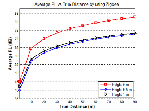
The results of the path losses are referred to as Figure 6, indicating that Wi-Fi has lower losses, especially when the Tx is at a height of 1 m.
Figure 6 discusses many points, the most important of which are:
1. Path Loss Characteristics Across Distances:
• It is anticipated that path loss escalates with increasing distance, as the attenuation of the signal intensifies over extended ranges.
• The graphical representation of Zigbee reveals marginally elevated initial path loss measurements at reduced distances in comparison to Wi-Fi, indicating that Zigbee may exhibit inferior performance under near-field conditions.
• At greater distances, Wi-Fi demonstrates superior attenuation management, as its overall PL values remain consistently lower than those of Zigbee for equivalent distances.
2. Influence of Antenna Elevation:
• Both communication technologies exhibit a significant correlation between antenna elevation and path loss.
• In measurements taken at ground level (illustrated by the red dashed line), both Zigbee and Wi-Fi incur the highest levels of signal degradation. Increasing the elevation to 0.5 m (represented by the blue dotted line) and subsequently to 1 m (depicted by the black solid line) enhances performance by minimizing the average path loss.
• Zigbee's responsiveness to variations in height appears to be more acute than that of Wi-Fi. The disparity between height levels is more pronounced for Zigbee, signifying its dependence on optimal placement for achieving peak performance.
3. Signal Consistency:
• The graph representing Wi-Fi displays a more gradual and less steep increase in path loss compared to Zigbee. This suggests that Wi-Fi may offer more reliable performance across a diverse spectrum of distances and elevations.
• Conversely, Zigbee exhibits somewhat erratic fluctuations, particularly at shorter distances, which may signify increased variability in signal integrity.
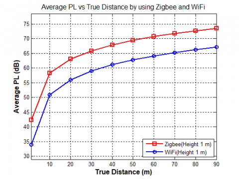
• A clear comparison of path loss between Wi-Fi and Zigbee at a height of Tx 1 m is referred to in Figure 7, which shows that Wi-Fi has path loss lower than Zigbee when the Tx height is 1 m and across distances from 1 m to 90 m, where the path loss for Wi-Fi at a distance of 90 m is 67.1 dB, while the path loss for Zigbee at the same distance is 73.5 dB, indicating that Wi-Fi has a lower loss rate of approximately 6.4 dB.
Which is superior?
In terms of performance, Wi-Fi is generally deemed superior for the following reasons:
1. Reduced Path Loss: Wi-Fi exhibits lower average path loss across various distances and elevations, indicating enhanced signal strength and reliability.
2. Enhanced Stability: The more gradual performance curve of Wi-Fi indicates greater consistency, rendering it a preferable option for contexts where reliability is paramount.
3. Insensitivity to Height: Although both technologies gain from elevated antenna positioning, Wi-Fi is less reliant on height modifications compared to Zigbee, thereby enhancing its adaptability.
Conversely, Zigbee may retain its benefits in particular situations, such as low-power Internet of Things (IoT) applications where energy efficiency is prioritized over signal robustness. Nonetheless, when evaluating overall communication quality and range, Wi-Fi surpasses Zigbee, according to the available data.
(a)
(b)
Figure 6. Results of the path losses: (a) Average path loss vs Distance by using Zigbee (b) Average path loss vs Distance by using Wi-Fi
Figure 7. Comparisons of path loss between Wi-Fi and Zigbee at a height of Tx 1 m
5.2 LNSM estimation model
The LNSM model and related parameters can be obtained by using average RSSI measurements from selected locations in outdoor environments. To determine the relevant parameters and the LNSM model illustrated in Table 1, consider the results of PL, the average RSSI, and the indisputable superiority of Wi-Fi, especially at a height of one meter.
Table 1. The significant factors of the LNSM framework for Zigbee and Wi-Fi at a height of 1 meter
|
Parameters |
Symbol |
Outdoor Environments |
|
|
Zigbee |
Wi-Fi |
||
|
PLE |
$\beta$ |
1.596354 |
1.695432 |
|
STD (dB) |
$\sigma$ |
7.813265 |
6.849800 |
|
Reference distance (m) |
$d_0$ |
1 |
1 |
|
Path loss at a distance (dBm) |
$P_L\left(d_0\right)$ |
42.28674 |
33.9502 |
|
Transmitter power (dBm) |
$P_t$ |
2 |
2 |
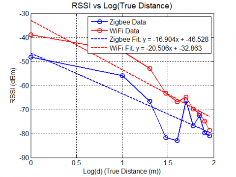
Figure 8 shows the relationship between the average RSSI values obtained at this 1-meter elevation and a logarithmic scale for the selected outdoor sites.
RSSI $($Zigbee$) =-16.904log \left(d / d_0\right)-46.528$ (7)
$R S S I(W i-F i)=-20.506 \log \left(d / d_0\right)-32.863$ (8)
Figure 8. The alignment of curves for an exterior setting
5.3 Errors and standard deviation estimation
Eqs. (7) and (8) serve as a tool to gauge the distance being examined relative to external surroundings, further elucidated in Eqs. (9) and (10).
$d_{\text {est }}($Zigbee$)=d_0 * 10^{-}\left(\frac{\text { RSSI }({Zigbee})+46.528}{16.904}\right)$ (9)
$d_{e s t}(W i-F i)=d_0 * 10^{-}\left(\frac{R S S I(W i-F i)+32.863}{20.506}\right)$ (10)
Utilizing Eqs. (9) and (10) allows us to derive the projected distance. The error in distance measurement can be assessed through Eqs. (11) and (12).
$e_i($Zigbee$)=d_{{true }}-d_{{est }}($Zigbee$)$ (11)
$e_i(W i-F i)=d_{{true }}-d_{{est }}(W i-F i)$ (12)
where, $d_{\text {true }}$ represents the authentic distance between a stationary node and a dynamic node, calculated using the conventional distance metric. $d_{e s t}$ refers to the observed (estimated) distance derived from Eqs. (9) and (10). Consequently, a distance measurement error can be illustrated as depicted in Figure 9. This illustration indicates that the error escalates with an increase in distance, showing a steady and gradual rise in scenarios involving a Wi-Fi network. The error also intensifies after 65 m. The figure indicates that the chosen measurement technique, namely LNSM, which relies on RSSI, proves to be effective in outdoor settings when the distance between fixed and mobile nodes is less than 65 m. The standard deviation of RSSI has been analyzed concerning distance, as demonstrated in Figure 10. This figure indicates that RSSI values vary more when they exceed 65 m for Wi-Fi, while for Zigbee, a significant deviation occurs beyond 20 m, leading to increased error when these thresholds are exceeded, as Figure 9 illustrates. Therefore, the results in Figure 10 are consistent with those in Figure 9.
Figure 9. Distance estimation error
Figure 10. Exploring the standard deviation of RSSI in relation to distance
It is important to highlight that the tests were conducted multiple times under comparable circumstances and at various times throughout the day, owing to the influence of weather patterns on the measurement values. These factors can be viewed as one of the challenges that lead to a notable fluctuation in the readings. Consequently, we have documented the average of STDs or the error margins for each distance derived from the repeated tests, as illustrated in Figure 10. This approach minimizes the impact of temporary environmental fluctuations and confirms the reliability and repeatability of the obtained results.
As shown in Figure 11, a linear regression was used to examine the relationship between actual and predicted distance. Based on the results, we know that for distances between 0 and 100 meters, the correlation coefficient for Zigbee was $R^2$= 0.19 and $R^2$= 0.22 for distances 0-65 m and 0-100 m, respectively, and for Wi-Fi, it was $R^2$= 0.91 and $R^2$= 0.86 for the same distances. If we compare Wi-Fi and Zigbee, we see that the correlation between actual and predicted distances is greater for Wi-Fi.
Figure 11. Linear regression relationship between true and estimated distance
5.4 MAE and RMSE
The discrepancy between the true distance and the estimated distance can be determined using MAE and RMSE. The formulas for MAE and RMSE can be derived from Eqs. (13) and (14), respectively [24].
$M A E=\frac{1}{n} \sum_{i=1}^n\left|e_i\right|$ (13)
$R M S E=\sqrt{\frac{1}{n} \sum_{i=1}^n e_i^2}$ (14)
where,
n represents the quantity of samples for the computed error. The MAE and RMSE error figures were derived as depicted in Figure 12 and Table 2, respectively. The calculations for MAE and RMSE indicate that distance measurement via LNSM demonstrates a commendable accuracy for shorter distances not exceeding 65 m for Zigbee, whereas it proves effective for longer distances up to 90 m for Wi-Fi, as the Wi-Fi error consistently remained lower than that of Zigbee, even over extended distances. Nevertheless, broadly speaking, for both methodologies, when the distance lies within the 0-65m range, the resulting error is superior compared to the 0-100m range.
Table 2 illustrates the advantages of our innovative system utilizing Wi-Fi technology. It achieved a reduced RMSE of 3.4 m and a diminished MAE of 0.86 m for distances 0-100 m, alongside a lower an MAE decrease of 1.7 m and lower RMSE of 8.66 m for distances 0-65 m in comparison to Proposed Zigbee.
Additionally, our cutting-edge Wi-Fi solution performs better than the previous two systems. Compared to study [8], it obtained a lower RMSE of 4.17 m and a decreased MAE of 5.78 m for 0-100 m, as well as a lower RMSE of 3.16 m and a decreased MAE of 3.11 m for 0-65 m.
Moreover, in juxtaposing the suggested Zigbee framework with study [8], we achieved a reduced MAE by 4.92 m and a diminished RMSE by 0.77 m for ranges of 0-100 m, along with a lower MAE by 1.41 m for distances spanning 0-65 m.
Ultimately, it’s important to highlight that our innovative Zigbee model achieved an RMSE that was 5.5 m higher for distances ranging from 0 to 65 m when contrasted with study [8]. Additionally, we observed that in our proposed framework, the RMSE for distances 0-65 m also surpassed that for distances 0-100 by 1.29 m. This phenomenon can be attributed to the multipath effect at shorter ranges, where signals bounce off the ground and arrive at the receiver via various routes (multiple paths). These reflections induce [constructive/destructive interference] in the signal, causing rapid fluctuations in the RSSI value, and Zigbee exhibits a heightened sensitivity to these environmental changes, particularly during close-range measurements. This is due to the minimal time difference between the paths, which significantly disrupts the original signal.
Figure 12. MAE and RMSE comparison
Table 2. RMSE and MAE of the systems
|
Model |
MAE (0-100m) |
RMSE (0-100m) |
MAE (0-65m) |
RMSE (0-65m) |
|
[8] |
6.72 m |
9.48 m |
3.44 m |
4.5 m |
|
Proposed Zigbee |
1.80 m |
8.71 m |
2.03 m |
10 m |
|
Proposed Wi-Fi |
0.94 m |
5.31 m |
0.33 m |
1.34 m |
Ultimately, the findings highlighted above showcase a distinct advantage of Wi-Fi over Zigbee regarding received signal strength (RSSI), RMSE, MAE, and $R^2$ values. Conversely, Zigbee excels in power efficiency, as it is a low-energy wireless communication solution designed for creating low-power wireless networks (LPWAN). Here lies the fundamental distinction between Wi-Fi and Zigbee when it comes to energy consumption.
The distance between the mobile units and the potential (stationary) Zigbee and Wi-Fi units in an outdoor environment was determined in this manuscript using the RSSI metrics of the mobile units. In order to create an external path loss model based on LNSM, a suitable linear correlation between the RSSI metrics and different distances was established. Additionally, channel metrics like PLE and STD were assessed. The RSSI STD was examined at various separations between mobile and stationary units. Notably, under comparable circumstances, the STD was more noticeable for Wi-Fi than Zigbee in the 0–90 m range. As a result, the RSSI variability increases as distance increases. After conducting an empirical evaluation in terrestrial settings, this study successfully deployed a reliable wireless communication technology. With Wi-Fi, a dependable and continuous connection was made possible, and a transmission distance of more than 90 meters between the transmitter and receiver was attained with tolerable path loss levels. By a margin of 6.4 dB, the effect of Wi-Fi network path losses was significantly less than that of Zigbee network path losses. This clear difference made it possible to use Wi-Fi to benefit from improved communication capabilities with low loss. The accuracy of estimating the distance between mobile and stationary nodes was evaluated using the correlation coefficient, MAE, and RMSE. The results show that Wi-Fi technology has a higher correlation coefficient than Zigbee. Moreover, the measurement was less than 65 meters. The RMSE was 1.34 m for Wi-Fi technology and 10 m for Zigbee technology, while the MAE was 2.03 m for Zigbee technology and 0.33 m for Wi-Fi technology. These results show that LNSM is a feasible solution for Wi-Fi networks up to 90 meters in length, with a lower error than Zigbee.
Future enhancements:
1. Investigating the impact of barriers like thick foliage to gain deeper insights into how signals behave in such settings, as well as to elucidate and comprehend the interference, scattering, and reflection of signals caused by these obstructions.
2. Incorporating precise numerical results to evaluate and contrast the overall energy usage between Zigbee and Wi-Fi by utilizing power measurement tools such as USB Power meters for accurate energy consumption assessments.
This work is supported by the College of Engineering/ Mustansi riyah University Iraq, Baghdad. https://www.uomustansiriyah.edu.iq/.
[1] Kurt, S., Tavli, B. (2017). Path-loss modeling for wireless sensor networks: A review of models and comparative evaluations. IEEE Antennas and Propagation Magazine, 59(1): 18-37. https://doi.org/10.1109/MAP.2016.2630035
[2] Kurt, S., Tavli, B. (2013). Propagation model alternatives for outdoor wireless sensor networks. In 2013 IFIP Wireless Days (WD), Valencia, Spain, pp. 1-3. https://doi.org/10.1109/WD.2013.6686515
[3] Mezaal, M.T., Aripin, N.B.M., Othman, N.S., Sallomi, A.H. (2024). The effect of urban environment on large-scale path loss model’s main parameters for mmWave 5G mobile network in Iraq. Open Engineering, 14(1): 20220601. https://doi.org/10.1515/eng-2022-0601
[4] Al-Mejibli, I., Mohammed, H.A., Hoomod, H.K., Alharbe, N.R. (2025). Path loss of indoor hotspot and indoor factory environments for 5G wireless networks. Journal of Engineering and Sustainable Development, 29(2): 170-176. https://doi.org/10.31272/jeasd.2473
[5] Hasan, M.Z., Mohd Hanapi, Z. (2023). Efficient and secured mechanisms for data link in IoT WSNs: A literature review. Electronics, 12(2): 458. https://doi.org/10.3390/electronics12020458
[6] Gherardi, F., Aquiloni, L. (2011). Sexual selection in crayfish: A review. In Proceedings of the TCS Summer Meeting, Tokyo, Japan, pp. 213-223. https://doi.org/10.1163/ej.9789004174252.i-354.145
[7] Malajner, M., Benkic, K., Planinsic, P., Cucej, Z. (2009). The accuracy of propagation models for distance measurement between WSN nodes. In 2009 16th International Conference on Systems, Signals and Image Processing, Chalkida, Greece, pp. 1-4. https://doi.org/10.1109/IWSSIP.2009.5367782
[8] Mohammed, S.L. (2016). Distance estimation based on RSSI and Log-Normal shadowing models for ZigBee wireless sensor network. Engineering and Technology Journal, 34(15): 2950-2959. https://doi.org/10.30684/etj.34.15a.15
[9] Zheng, J., Wu, C., Chu, H., Xu, Y. (2011). An improved RSSI measurement in wireless sensor networks. Procedia Engineering, 15: 876-880. https://doi.org/10.1016/j.proeng.2011.08.162
[10] Chen, Z., Fu, X., Kong, Y., Han, D. (2014). Study on path loss of ZigBee signal in electrical substation environment. In International Conference on Cyberspace Technology (CCT 2014), Stevenage UK: IET, p. 44. https://doi.org/10.1049/cp.2014.1323
[11] Wu, H., Zhang, L., Miao, Y. (2017). The propagation characteristics of radio frequency signals for wireless sensor networks in large-scale farmland. Wireless Personal Communications, 95(4): 3653-3670. https://doi.org/10.1007/s11277-017-4018-5
[12] Benkič, K., Malajner, M., Planinsic, P., Cucej, Z. (2008). Using RSSI value for distance estimation in wireless sensor networks based on ZigBee. In 2008 15th International Conference on Systems, Signals and Image Processing, Bratislava, Slovakia, pp. 303-306. https://doi.org/10.1109/IWSSIP.2008.4604427
[13] Supreeth, N.M., Akhil, K.M. (2025). Location verification of wireless sensor node using integrated trilateration in Outdoor WSN. Procedia Computer Science, 252: 567-575. https://doi.org/10.1016/j.procs.2025.01.016
[14] Mowla, M.N., Mowla, N., Shah, A.S., Rabie, K.M., Shongwe, T. (2023). Internet of Things and wireless sensor networks for smart agriculture applications: A survey. IEEE Access, 11: 145813-145852. https://doi.org/10.1109/ACCESS.2023.3346299
[15] Farooq, M.S., Riaz, S., Helou, M.A., Khan, F.S., Abid, A., Alvi, A. (2022). Internet of things in greenhouse agriculture: A survey on enabling technologies, applications, and protocols. IEEE Access, 10: 53374-53397. https://doi.org/10.1109/ACCESS.2022.3166634
[16] García, L., Viciano-Tudela, S., Sendra, S., Lloret, J. (2022). Practical design of a WiFi-based wireless sensor network for precision agriculture in citrus crops. In Proceedings of the 19th International Conference on Wireless Networks and Mobile Systems (WINSYS 2022), Lisbon, Portugal, pp. 107-114. https://doi.org/10.5220/0011355300003286
[17] Tang, P., Liang, Q., Li, H., Pang, Y. (2024). Application of internet-of-things wireless communication technology in agricultural irrigation management: A review. Sustainability, 16(9): 3575. https://doi.org/10.3390/su16093575
[18] Jindarat, S., Wuttidittachotti, P. (2015). Smart farm monitoring using Raspberry Pi and Arduino. In 2015 International Conference on Computer, Communications, and Control Technology (I4CT), Kuching, Malaysia, pp. 284-288. https://doi.org/10.1109/I4CT.2015.7219582
[19] Li, H., Zhao, L., Darr, M.J., Ling, P. (2009). Modeling wireless signal transmission performance path loss for ZigBee communication protocol in residential houses. American Society of Agricultural and Biological Engineers. https://doi.org/10.13031/2013.27227
[20] Musikanon, O., Chongburee, W. (2012). ZigBee propagations and performance analysis in lastmile network. International Journal of Innovation, Management and Technology, 3(4): 353-357. http://doi.org/10.7763/IJIMT.2012.V3.253
[21] Shojaifar, A. (2015). Evaluation and improvement of the RSSI-based localization algorithm: Received signal strength indication (RSSI). Computer Science, Engineering.
[22] Ta, X., Mao, G., and Anderson, B.D.O. (2009). On the giant component of wireless multihop networks in the presence of shadowing. IEEE Transactions on Vehicular Technology, 58(9): 5152-5163. https://doi.org/10.1109/TVT.2009.2026480
[23] Aramice, G.A., Miry, A.H., Salman, T.M. (2023). Optimal long-range-wide-area-network parameters configuration for internet of vehicles applications in suburban environments. Journal of Engineering and Sustainable Development, 27(6): 754-770. https://doi.org/10.31272/jeasd.27.6.7
[24] Chai, T., Draxler, R.R. (2014). Root mean square error (RMSE) or mean absolute error (MAE)?–Arguments against avoiding RMSE in the literature. Geoscientific model Development, 7(3): 1247-1250. https://doi.org/10.5194/gmd-7-1247-2014