Tran Dong*![]() | Vu Thi To Linh
| Vu Thi To Linh![]()
© 2025 The authors. This article is published by IIETA and is licensed under the CC BY 4.0 license (http://creativecommons.org/licenses/by/4.0/).
OPEN ACCESS
In today's energy sector, wind power has risen to prominence as a key renewable resource, appreciated for its eco-friendliness, sustainability, and minimal environmental footprint. Over recent decades, its adoption has surged, making it the fastest-growing option among renewable energy sources. Wind energy is captured and transformed into electricity via Wind Energy Conversion Systems (WECS), which predominantly rely on wind turbines. WECS can be divided into two main categories based on their interaction with power grids: grid-connected systems and stand-alone wind energy systems. Currently, most wind energy installations are grid-connected, facilitating efficient integration and distribution of the generated electricity. The control systems for WECS are intricate, necessitating advanced optimization methods to improve the effectiveness of wind energy conversion. This paper introduces an innovative approach to crafting an adaptive optimal controller based on Adaptive Dynamic Programming (ADP), aimed at enhancing energy conversion efficiency for grid-connected wind energy systems that use Permanent Magnet Synchronous Generators (PMSG). The proposed controller leverages reinforcement learning techniques along with Lyapunov stability analysis to guarantee dependable performance across a range of operational scenarios. To demonstrate the controller's effectiveness, we implemented and simulated a complete system comprising both the WECS and the controller in the Matlab and Simulink environments. The outcomes of these simulations will be evaluated to determine the controller's performance and its potential to boost the overall operational efficiency of wind energy systems.
wind energy conversion systems, permanent magnet synchronous generators, adaptive dynamic programming, lyapunov theory
Wind energy is a very important research field nowadays, especially in the context of the world's efforts to switch to renewable energy sources to replace increasingly depleted conventional energy sources. WECS consist of many aerodynamic, mechanical and electrical components. The performance of this system depends on several important factors, including the installation location, wind speed and especially the type of generator. Among these factors, wind speed is continuously variable during operation, while other factors are usually precisely determined during the design and construction phase.
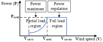
In a wind turbine system, the operational phases are categorized into two primary areas: the partial load region and the full load region, as illustrated in Figure 1.
The partial load region refers to the operational state where the wind turbine functions below its rated capacity. During this phase, the turbine's efficiency is hindered by insufficient wind or other conditions that limit power output. This region typically occurs under low or fluctuating wind conditions, necessitating adjustments to the blade pitch to enhance performance. Conversely, the full load region represents the state in which the wind turbine achieves its maximum power output. In this phase, the turbine is finely tuned to capture wind energy most effectively. This operational region is reached when wind speeds are consistently high and stable, enabling the turbine to perform at its best.
Figure 1. Partial load region and full load region of wind turbine
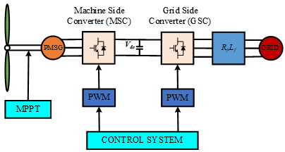
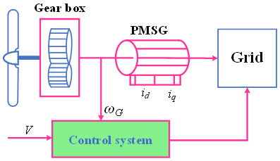
Modeling and control in WECS focus on exploiting the dynamic characteristics of wind turbines and designing optimal control systems to increase energy production. This process typically involves analyzing the dynamic characteristics of PMSG, as well as implementing control strategies to improve the stability and efficiency of the system. This is essential to ensure efficient and reliable operation of WECS. Modeling of wind turbines can be performed through simulation methods, which allow analysis of their static and dynamic characteristics, thereby optimizing performance and evaluating feasibility under different conditions. Current research also focuses on the control architecture of these systems, including blade regulation and drive mechanisms [1, 2]. In wind turbine control, various methods are applied, including conventional, nonlinear, and intelligent control methods. Proportional-Integral-Derivative (PID) control is one of the most common methods in the industry. PID regulates the rotational speed of the turbine through three components: proportional (P), integral (I), and derivative (D), to maintain a stable rotational speed and minimize errors [3, 4]. In the study [3], a new design procedure for a decoupled PI controller for a wind turbine using a PMSG is presented. The findings demonstrate that the proposed method successfully recovers nominal performance levels, even in the presence of model uncertainties, while simultaneously enhancing performance during the transient phase of operation. In contrast, Tripathi et. al [4] emphasizes the evaluation of a wind turbine control system that employs Permanent Magnet Synchronous Generators (PMSG). This study specifically highlights the significance of tuning the Proportional-Integral (PI) controller parameters, with a focus on achieving a desired damping ratio. Such tuning is essential for enhancing both the performance and stability of the system under various real-world operating conditions. Moreover, adaptive control mechanisms offer a promising solution by automatically adjusting controller parameters over time in response to changing operating conditions or fluctuations in turbine dynamics, as noted in references [5, 6]. Although this approach necessitates a precise model of the system, it has the potential to significantly improve performance, particularly under unstable conditions. In reference [5], a novel adaptive control strategy is introduced, aimed at enhancing the performance of small wind turbines equipped with PMSGs operating in region II. This method utilizes a reference model to fine-tune control parameters, thereby optimizing energy efficiency while ensuring that the system remains within operational limits. Reference [6] provides an analysis of the performance of a wind turbine system using adaptive dynamic range control. This innovative control technique is primarily applied to power converters, resulting in improved performance and responsiveness in handling grid energy generated from wind turbines. Overall, these studies contribute valuable insights into the optimization of wind turbine control systems, highlighting the effectiveness of adaptive strategies in ensuring robust and efficient energy production. This can lead to better operating efficiency and minimize power fluctuations. Optimal control uses real-time algorithms to optimize the blade angle and rotation speed with the goal of achieving maximum efficiency [7, 8]. In the study [7], the optimal control methods for WECS are reviewed, focusing on power optimization and multi-purpose criteria. It aims to provide an overview of different control methods aimed at optimizing the dynamic behavior of multi-speed wind turbines. In the study [8], an optimal strategy for controlling and operating wind turbines to provide frequency support to the grid was proposed. This strategy is implemented through the development of frequency support capabilities of permanently synchronous generators (PMSG) connected to the power system. It includes controlling the active power to participate in the frequency regulation of the grid. In the study [9], an optimal strategy for operating wind farms to maintain frequency regulation reserve, considering wake effects, was proposed. This study focuses on the trade-off between power output and frequency regulation reserve capacity of wind farms. In the study [10], an optimal strategy for operating wind farms to maintain frequency regulation reserve, considering wake effects, was proposed. This study focuses on the trade-off between power output and frequency regulation reserve capacity of wind farms. Robust control of WECS is designed to withstand large wind variations, network disturbances, and parameter uncertainties [11-13]. Several studies have developed robust control algorithms and implemented these techniques using hardware such as FPGAs [14, 15]. These approaches aim to increase the reliability and performance of WECS under unstable operating conditions. Research on fuzzy control or neural networks and adaptive control allows turbines to adjust to changing wind conditions [16-21]. These methods are capable of handling uncertainties and nonlinearities in the behavior of wind turbines. Using fuzzy logic rules, the system can make decisions based on imprecise values. In the study [18] presents a Takagi-Sugeno (T-S) fuzzy control system for a Wind Energy Conversion System (WECS) utilizing a Permanent Magnet Synchronous Generator (PMSG), designed through the Linear Matrix Inequality (LMI) method. This approach optimizes system stability and performance under uncertain conditions, leveraging the flexibility of fuzzy control and logic rules to precisely meet design criteria. Additionally, recent research explores machine learning techniques to enhance wind turbine control by enabling models to learn from real data and improve their performance [22-25]. Each method has unique advantages and drawbacks, making it crucial to select the right approach based on the system’s specific needs and operating environment. Moreover, intelligent control methods utilizing reinforcement learning are being developed to optimize operational efficiency. Techniques such as torque control and multiple-input-multiple-output (MIMO) systems have been enhanced with advanced reinforcement learning algorithms to improve wind energy extraction, particularly in response to fluctuating wind speeds, thereby boosting the efficiency of PMSG-based systems. This paper combines these control strategies, employing neural networks for system state estimation and designing a controller based on the Adaptive Dynamic Programming (ADP) technique to optimize output power and enhance stability amid changing wind conditions. The overall WECS model is illustrated in Figure 2.
Figure 2. Overall model of WECS
This section will present the dynamic modeling process of the WECS. The modeling will be performed for each subsystem, and then the models of these subsystems will be combined into a nonlinear model of the entire WECS. The WECS consists of many different physical components. These systems can be divided into two different groups: the electrical components group and the mechanical components group. In terms of dynamics, the WECS consists of four types of dynamics: the aerodynamics of the rotor, the structural dynamics of the blades and turbine tower, the dynamics of the drive, and the dynamics of the generator. The block diagram of the WECS modeling is shown in Figure 3. However, in terms of control objectives, only the dynamics of the rotor, drive, and generator are modeled.
Figure 3. Block diagram of WECS modeling
2.1 Aerodynamic modeling of wind turbines
Figure 4 illustrates the aerodynamic model of a wind turbine. Its main role is to convert the energy from the wind into mechanical energy for the turbine.
Figure 4. Aerodynamics of wind turbines
When the wind moves through the turbine's sweep area, it produces forces that impact the turbine. These forces include the thrust force acting on the shaft and blades, along with the torque that drives the rotor's rotation. The thrust force $F_T$, the torque $T_R$, and the mechanical power $P_R$ generated are defined as follows [26, 27]:
$F_T=\frac{1}{2} \rho \pi R^3 V^2 C_T(\lambda, \beta)$ (1)
$T_R=\frac{1}{2} \rho \pi R^3 V^2 C_Q(\lambda, \beta)$ (2)
$P_R=\frac{1}{2} \rho \pi R^2 V^3 C_P(\lambda, \beta)$ (3)
where, $\rho$ represents the air density, $R$ denotes the swept radius, $V$ indicates the wind speed, $C_Q(\lambda, \beta)$ refers to the torque coefficient, and $C_P(\lambda, \beta)$ signifies the power conversion coefficient. Both the torque and mechanical power are influenced by the tip-speed ratio (TSR) $\lambda$ and the pitch angle $\beta$. The TSR $\lambda$ is defined as the ratio of the velocity of the blade tips to the wind speed:
$\lambda=\frac{\omega_R R}{V}$ (4)
where, $\omega_R$ represents the rotor's angular velocity. The connection between the torque coefficient and the power coefficient is defined as follows:
$C_P(\lambda, \beta)=\lambda C_Q(\lambda, \beta)$ (5)
2.2 Dynamic modeling of the drive system
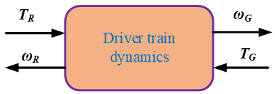
The primary role of the drive is to convey mechanical energy from the rotor to the generator. Figure 5 shows a block diagram of the drive. In this system, the input signals consist of the torques from both the turbine and the generator, while the output signals represent the angular velocities of these components.
Figure 5. Block diagram of the drive
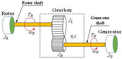
Depending on the control purpose, the drive can be modeled as a rigid or elastic model. For small-capacity wind power systems, to simplify the modeling process, a rigid model is often used to describe the drive dynamics. This rigid model is illustrated in Figure 6.
Figure 6. Rigid model of the actuator
The rigid model of the drive consists of two rigid shafts connected to each other through a velocity multiplier. These rigid shafts include the shaft connected to the rotor receiving the turbine torque $T_R$, with a low velocity $\omega_R$, and the shaft connected to the generator receiving the generator torque $T_G$, with a high velocity $\omega_G$. The rotor and the generator are considered as rigid bodies with moments of inertia $J_R$ and $J_G$ respectively. The velocity multiplier consists of two gears with inertias $J_L$ and $J_H$ respectively, with a velocity conversion efficiency $\eta$ and a velocity receiving ratio $i$. The dynamics of this model can be described by a first-order differential equation converted to the generator side as follows [26]:
$\dot{\omega}_G=\frac{\eta}{i J_h} T_R-\frac{1}{J_h} T_G$ (6)
where, $J_h$ is the equivalent torque converted to the generator side and is calculated as follows:
$J_h=\left(J_L+J_R\right) \frac{\eta}{i^2} T_R+J_H+J_G$ (7)
If converted to the turbine side, the kinematic equation of the drive can be written as follows:
$\dot{\omega}_R=\frac{1}{I_1} T_R-\frac{i}{\eta I_1} T_G$ (8)
where, $J_l$ is the equivalent moment converted to the turbine side and is calculated as follows:
$J_l=\left(J_H+J_G\right) \frac{i^2}{\eta}+J_L+J_R$ (9)
2.3 Modeling of PMSG
The control structure for WECS is divided into many control loops to ensure stable and continuous power supply to loads and grid connection. In this section, we only focus on designing a controller to optimize the energy conversion process for wind turbines, so we only model the dynamics of the wind turbine, drive and generator as shown in Figure 7.
Figure 7. WECS model
The type of generator commonly used in WECS is the PMSG. The mathematical model of the PMSG generator in the d, q coordinate system is given as follows [3, 26, 27]:
$\left\{\begin{array}{c}\frac{d i_d}{d t}=-\frac{R_s}{L_d} i_d+\frac{p L_q}{L_d} i_q \omega_G-\frac{1}{L_d} u_d \\ \frac{d i_q}{d t}=-\frac{R_s}{L_q} i_q-\frac{p}{L_q}\left(L_d i_d-\phi_m\right) \omega_G-\frac{1}{L_q} u_q\end{array}\right.$ (10)
where, $i_d, \, i_q$ are the stator current $d, \, q; \, u_d, u_q$ are the stator input voltage $d, \, q; \, L_d, L_q$ are the stator inductance $d, \, q; \, R_s$ is the stator resistance; $p$ is the number of pole pairs; $\phi_m$ is the magnetic flux; $\omega_G$ is the generator speed.
2.4 Dynamic model of WECS
By integrating the dynamics of the wind turbine, drive, and generator discussed earlier, we derive the dynamic model of the WECS utilizing a PMSG as follows [3]:
$\left\{\begin{array}{c}\dot{\omega}_G=\frac{\eta}{i J_h} T_R-\frac{1}{J_h} p \phi_m i_q \\ \frac{d i_d}{d t}=-\frac{R_s}{L_d} i_d+\frac{p L_q}{L_d} i_q \omega_G-\frac{1}{L_d} u_d \\ \frac{d i_q}{d t}=-\frac{R_s}{L_q} i_q-\frac{p}{L_q}\left(L_d i_d-\phi_m\right) \omega_G-\frac{1}{L_q} u_q\end{array}\right.$ (11)
where, $T_G=p \phi_m i_q$
Let the state variable vector $x=\left[\begin{array}{lll}x_1 & x_2 & x_3\end{array}\right]^T$, where $x_1=\omega_{r e f}-\omega_G ; x_2=i_{d r e f}-i_d ; x_3=i_{q r e f}-i_q$.
$\begin{gathered}\Rightarrow \dot{x}=\left[\begin{array}{c}\dot{x}_1 \\ \dot{x}_2 \\ \dot{x}_3\end{array}\right]=\left[\begin{array}{c}\dot{\omega}_{\text {ref }}-\dot{\omega}_G \\ \tilde{l}_{\text {dref }}-\tilde{l}_d \\ \tilde{l}_{\text {qref }}-\tilde{l}_q\end{array}\right] \\ =\left[\begin{array}{c}\dot{\omega}_{\text {ref }}-\frac{\eta}{i J_h} T_R+\frac{1}{J_h} p \phi_m i_q \\ \tilde{l}_{\text {dref }}+\frac{R_s}{L_d} i_d-\frac{p L_q}{L_d} i_q \omega_G+\frac{1}{L_d} u_d \\ \tilde{l}_{\text {qref }}+\frac{R_s}{L_q} i_q+\frac{p}{L_q}\left(L_d i_d-\phi_m\right) \omega_G+\frac{1}{L_q} u_q\end{array}\right]\end{gathered}$ (12)
The dynamic model (12) is written as follows:
$\left\{\begin{array}{c}\dot{x}=\mathcal{F}(x, u) \\ y=\mathcal{C} x\end{array}\right.$ (13)
where, $F(x, u)=\left[\begin{array}{c}\dot{\omega}_{\text {ref }}-\frac{\eta}{i_{J h}} T_R+\frac{1}{J_h} p \phi_m i_q \\ \tilde{\imath}_{\text {dref }}+\frac{R_s}{L_d} i_d-\frac{p L_q}{L_d} i_q \omega_G+\frac{1}{L_d} u_d \\ \tilde{\imath}_{\text {qref }}+\frac{R_s}{L_q} i_q+\frac{p}{L_q}\left(L_d i_d-\phi_m\right) \omega_G+\frac{1}{L_q} u_q\end{array}\right];$ $u=\left[\begin{array}{l}u_d \\ u_q\end{array}\right]$ is the control signal vector.
3.1 ADP based controller design
In this section, we develop a controller using the ADP method to enhance the energy conversion process for the WECS. For optimal output control problems, the goal is to design an optimal controller for system (13) to minimize the infinite cost function [28].
$\mathcal{V}(x)=\int_t^{\infty}\left(u^T \mathcal{R} u+y^T \mathcal{Q} y\right) d t$ (14)
where, $Q$ and $\mathcal{R}$ are positive definite matrices.
Since the state of the system is unknown, we will use a state observer to estimate these states. From Eq. (13) we have:
$\left\{\begin{array}{c}\dot{x}=\mathcal{A} x+\mathcal{B}(x, u) \\ y=\mathcal{C} x\end{array}\right.$ (15)
where, $\mathcal{B}(x, u)=\mathcal{F}(x, u)-\mathcal{A} x ; \mathcal{A}$ is the Hurwit matrix, the system (15) is completely observable.
Using the state observer, the system (15) is represented as:
$\left\{\begin{array}{c}\dot{\hat{x}}=\mathcal{K}(y-\mathcal{C} \hat{x})+\mathcal{A} \hat{x}+\mathcal{B}(\hat{x}, u) \\ \hat{y}=\mathcal{C} \hat{x}\end{array}\right.$ (16)
where, $\hat{x}$ is the state of the observer; $\hat{y}$ is the output of the observer; $\mathcal{A}-\mathcal{K} \mathcal{C}$ is the Hurwitz matrix.
$\mathcal{B}(x, u)$ is an undefined nonlinear function. To calculate the value of $\mathcal{B}(x, u)$, we use the following neural network:
$\mathcal{B}(x, u)-\varepsilon_0(x)=\mathcal{W}_2^T \phi\left(\mathcal{W}_1^T \underline{x}\right)$ (17)
$\underline{x}=\left[\begin{array}{l}x^T \\ u^T\end{array}\right]$ represents the input to the $\mathrm{NN} ; \phi($.$) denotes the$ activation function of the $\mathrm{NN}; \,\varepsilon_0(x)$ signifies the approximation error associated with the bounded NN function; $\mathcal{W}_1$ refers to the optimal weight matrix connecting the input layer to the hidden layer, while $\mathcal{W}_2$ stands for the optimal weight matrix linking the hidden layer to the output layer.
The ideal weights of the neural network are unknown so $\mathcal{B}(x, u)$ is approximated by
$\begin{gathered}\widehat{\mathcal{B}}(\hat{x}, u)=\widehat{\mathcal{W}}_2^T \phi\left(\widehat{\mathcal{W}}_1^T \widehat{x}\right) \\ \underline{\hat{x}}=\left[\begin{array}{l}\hat{x}^T \\ u^T\end{array}\right]\end{gathered}$ (18)
where, $\hat{x}$ is the estimated state vector; $\widehat{\mathcal{W}}_1, \widehat{\mathcal{W}}_2$ are the estimated weight matrices.
Then Eq. (16) is rewritten as follows:
$\left\{\begin{array}{c}\hat{x}=\mathcal{K}(y-\mathcal{C} \hat{x})+\mathcal{A} \hat{x}+\widehat{\mathcal{W}}_2^T \phi\left(\widehat{\mathcal{W}}_1^T \hat{x}\right) \\ \hat{y}=\mathcal{C} \hat{x}\end{array}\right.$ (19)
Let $\tilde{x}=x-\hat{x}$ be the state estimation error; $\tilde{y}=y-\hat{y}$ be the output estimation error, we have:
$\left\{\begin{array}{c}\dot{\tilde{x}}=\mathcal{W}_2^T \phi\left(\mathcal{W}_1^T \underline{x}\right)+(\mathcal{A}-K C) \tilde{x} \\ -\widehat{\mathcal{W}}_2^T \phi\left(\widehat{\mathcal{W}}_1^T \underline{x}\right)+\varepsilon_0(x) \\ \tilde{y}=C \tilde{x}\end{array}\right.$ (20)
Let $\quad \widetilde{\mathcal{W}}_2=\mathcal{W}_2-\widehat{\mathcal{W}}_2, \quad \mathcal{D}=\mathcal{A}-\mathcal{K} \mathcal{C}, \quad \delta(x)=$ $\mathcal{W}_2^T\left[\phi\left(\mathcal{W}_1^T \underline{x}\right)-\phi\left(\widehat{\mathcal{W}}_1^T \underline{\hat{x}}\right)\right]+\varepsilon_0(x)$, Eq. (19) becomes:
$\left\{\begin{array}{c}\dot{\tilde{x}}=\mathcal{D} \tilde{x}+\delta(x)+\widetilde{\mathcal{W}}_2^T \phi\left(\widehat{\mathcal{W}}_1^T \hat{x}\right) \\ \tilde{y}=\mathcal{C} \tilde{x}\end{array}\right.$ (21)
Then we have the Hamilton function:
$\mathcal{H}\left(\hat{x}, u, v_{\hat{x}}\right)=r(\hat{x}, u)+v_{\hat{x}}^T \mathcal{F}(\hat{x}, u)$ (22)
where, $r(\hat{x}, u)=u^T \mathcal{R} u+\hat{x}^T Q \hat{x}$
The optimal value function is:
$\mathcal{V}^*(\hat{x})=\min \int_t^{\infty} r(\hat{x}, u) d t$ (23)
$\mathcal{V}^*(\hat{x})$ satisfies the HJB equation:
$\min \mathcal{H}\left(\hat{x}, u, \mathcal{V}_{\hat{x}}^*\right)=0$ (24)
where, $V_{\hat{x}}^*=\frac{\partial \mathcal{V}^*(\hat{x})}{\partial \hat{x}}$
From there we have the optimal controller:
$u^*=-\frac{1}{2} \mathcal{R}^{-1}\left(\frac{\partial \mathcal{F}(\hat{x}, u)}{\partial u}\right)^T \nu_{\hat{x}}^*$ (25)
The value function is computed by a neural network called a Critic neural network.
$\mathcal{V}^*(\hat{x})=\varepsilon_c(\hat{x})+\mathcal{W}_c^T \phi\left(\mathcal{W}_{c 1}^T \hat{x}\right)$ (26)
where, $\mathcal{W}_c$ is the ideal weight matrix for the hidden layer to the output layer, $\mathcal{W}_{c1}$ is the ideal weight matrix for the input layer to the hidden layer of the Critic neural network.
The output of the Critic neural network is calculated as follows:
$\widehat{v}(\hat{x})=\widehat{w}_r^T \phi\left(\mathcal{W}_{c 1}^T \hat{x}\right)=\widehat{w}_c^T \phi(z)$ (27)
where, $\widehat{\mathcal{W}}_c$ is the estimated weight matrix of $\mathcal{W}_c, z=\mathcal{W}_{c 1}^T \hat{x}$.
The Hamiltonian function is approximated by the equation:
$\mathcal{H}\left(\widehat{x}, u, \widehat{\mathcal{W}}_c\right)=r(\widehat{x}, u)+\widehat{\mathcal{W}}_c^T \nabla \phi \mathcal{F}(\widehat{x}, u)=e_c$ (28)
$\Rightarrow e_c=r(\hat{x}, u)+\widehat{\mathcal{W}}_c^T \nabla \phi \dot{\hat{x}}=e_c$ (29)
The Critic neural network weight update rule is calculated as follows:
$\dot{\widehat{{W}}}_c=-\alpha \frac{\varphi}{\left(\varphi^T \varphi+1\right)^2}\left(\varphi^T \widehat{\mathcal{W}}_c+r(\hat{x}, u)\right)$ (30)
Then the control law is approximated as follows:
$\hat{u}=-\frac{1}{2} \mathcal{R}^{-1}\left(\frac{\partial \hat{\mathcal{F}}(\hat{x}, u)}{\partial u}\right)^T \nabla \phi^T \widehat{W}_c$ (31)
3.2 Proving the stability of closed loop systems
Consider the stability of closed-loop systems using Lyapunov candidate functions [28].
$\begin{gathered}\mathcal{L}(x)=\frac{1}{2 \alpha} \widetilde{\mathcal{W}}_c^T \widetilde{\mathcal{W}}_c+\alpha\left(x^T x+\beta \mathcal{V}(x)\right)+\frac{1}{2} \tilde{x}^T \mathcal{P} \tilde{x} \\ +\frac{1}{2} \operatorname{tr}\left(\widetilde{\mathcal{W}}_1^T \widetilde{\mathcal{W}}_1\right)+\frac{1}{2} \operatorname{tr}\left(\widetilde{\mathcal{W}}_2^T \widetilde{\mathcal{W}}_2\right)\end{gathered}$
First derivative of Lyapunov function we have:
$\begin{aligned} \dot{\mathcal{L}}=\frac{1}{\alpha} \widetilde{\mathcal{W}}_c^T \dot{\tilde{\mathcal{W}}}_c+ & 2 \alpha x^T \dot{x}+\alpha \gamma\left(-x^T Q_c x-\hat{u}^T \mathcal{R} \hat{u}\right)-\frac{\rho}{2} \tilde{x}^T \tilde{x} \\ & +\tilde{x} \mathcal{P}\left(\widetilde{\mathcal{W}}_2^T \phi\left(\widehat{\mathcal{W}}_1^T \hat{x}\right)+\zeta\right) \\ & +\operatorname{tr}\left\{\widetilde{\mathcal{W}}_1^T \operatorname{sgn}\left(\underline{\hat{x}}^T\right) \tilde{y}^T l_2 \widehat{\mathcal{W}}_2^T\left(I_k-\sigma\left(\widehat{\mathcal{W}}_1^T \underline{\hat{x}}\right)\right)\right. \\ & \left.+\widetilde{\mathcal{W}}_1^T \theta_2\|\tilde{y}\|\left(\mathcal{W}_1-\widetilde{\mathcal{W}}_1\right)\right\} \\ & +\operatorname{tr}\left\{\widetilde{\mathcal{W}}_2^T \phi\left(\widehat{\mathcal{W}}_1^T \underline{\hat{x}}\right) \tilde{y}^T l_1\right. \\ & \left.+\widetilde{\mathcal{W}}_2^T \theta_1\|\tilde{y}\|\left(\mathcal{W}_1-\widetilde{\mathcal{W}}_1\right)\right\}\end{aligned}$
$\begin{aligned} \dot{\mathcal{L}}= & \frac{1}{\alpha} \widetilde{\mathcal{W}}_c^T\left(\alpha \psi_1 \frac{\vartheta}{\psi_2}-\alpha \psi_1 \psi_1^T \widetilde{\mathcal{W}}_c\right) \\ & +2 \alpha x^T\left(\mathcal{A} x+\mathcal{W}_2^T \phi\left(\mathcal{W}_1^T \underline{x}\right)+\varepsilon\right) \\ & +\alpha \gamma\left(-x^T Q_c x-\hat{u}^T \mathcal{R} \hat{u}\right)-\frac{\rho}{2} \tilde{x}^T \tilde{x} \\ & +\operatorname{tr}\left\{\widetilde{\mathcal{W}}_1^T \operatorname{sgn}(\underline{\hat{x}}) \tilde{y}^T l_2 \widehat{\mathcal{W}}_2^T\left(I_k-\sigma\left(\widehat{\mathcal{W}}_1^T \underline{\hat{x}}\right)\right)\right. \\ & \left.+\widetilde{\mathcal{W}}_1^T \theta_2\|\tilde{y}\|\left(\mathcal{W}_1-\widetilde{\mathcal{W}}_1\right)\right\} \\ & +\tilde{x} \mathcal{P}\left(\widetilde{\mathcal{W}}_2^T \phi\left(\widehat{\mathcal{W}}_1^T \hat{x}\right)+\zeta\right) \\ & +\operatorname{tr}\left\{\widetilde{\mathcal{W}}_2^T \phi\left(\widehat{\mathcal{W}}_1^T \hat{x}\right) \tilde{y}^T l_1\right. \\ & \left.+\widetilde{\mathcal{W}}_2^T \theta_1\|\tilde{y}\|\left(\mathcal{W}_1-\mathcal{W}_1\right)\right\}\end{aligned}$
$\begin{aligned} \Rightarrow \dot{\mathcal{L}} \leq \widetilde{\mathcal{W}}_c^T \psi_1 \frac{\vartheta}{\psi_2} & -\left\|\widetilde{\mathcal{W}}_c^T \psi_1\right\|^2 \\ & +\alpha\left[x^T x\right. \\ & +\left(\mathcal{A} x+\mathcal{W}_2^T \phi\left(\mathcal{W}_1^T \underline{x}\right)+\varepsilon\right)^T(\mathcal{A} x \\ & \left.+\mathcal{W}_2^T \phi\left(\mathcal{W}_1^T \underline{x}\right)+\varepsilon\right) \\ & \left.+\gamma\left(-x^T Q_c x-\hat{u}^T \mathcal{R} \hat{u}\right)\right] \\ & +\left[\zeta_M\|\mathcal{P}\|\|\mathcal{C}\|+\left(\theta_1-\mathcal{K}_1^2\right) \mathcal{K}_2^2\right. \\ & +\left(\theta_2-1\right) K_3^2-\left(\theta_1-\mathcal{K}_1^2\right)\left(\mathcal{K}_2-\left\|\tilde{\mathcal{W}}_1\right\|\right)^2 \\ & -\left(\theta_2-1\right)\left(\mathcal{K}_3-\left\|\tilde{\mathcal{W}}_2\right\|\right)^2 \\ & \left.-\left(\mathcal{K}_1\left\|\tilde{\mathcal{W}}_1\right\|-\left\|\tilde{\mathcal{W}}_2\right\|\right)^2\right]\|\tilde{y}\| \\ & -\frac{\rho}{2} \lambda_{\min }\left[(\mathcal{C})^T \mathcal{C}\right]\|\tilde{y}\|^2\end{aligned}$
$\begin{aligned} \dot{\mathcal{L}} \leq\left\|\widetilde{\mathcal{W}}_c^T \psi_1\right\| \| & \frac{\vartheta}{\psi_2}\|-\| \widetilde{\mathcal{W}}_c^T \psi_1\left\|^2-\frac{\rho}{2} \lambda_{\min }\left[(\mathcal{C})^T \mathcal{C}\right]\right\| \tilde{y} \|^2 \\ & +d\|\tilde{y}\| \\ & +\alpha\left[\left(1+3\|\mathcal{A}\|^2\right)\|x\|^2\right. \\ & +3\left\|\mathcal{W}_2^T \phi\left(\mathcal{W}_1^T \underline{x}\right)\right\|^2+3\|\varepsilon\|^2 \\ & \left.-\gamma \lambda_{\min }\left(Q_c\right)\|x\|^2-\gamma \lambda_{\min }(\mathcal{R})\|\hat{u}\|^2\right]\end{aligned}$
$\begin{aligned} \dot{\mathcal{L}} \leq\left\|\widetilde{\mathcal{W}}_c^T \psi_1\right\| \vartheta_M & -\left\|\widetilde{\mathcal{W}}_c^T \psi_1\right\|^2-\frac{\rho}{2} \lambda_{\min }\left[(\mathcal{C})^T \mathcal{C}\right]\|\tilde{y}\|^2 \\ & +d\|\tilde{y}\| \\ & -\alpha\left[\left(\lambda_{\min }\left(Q_c\right)\right)-1-3\|\mathcal{A}\|^2\|x\|^2\right. \\ & \left.-\gamma \lambda_{\min }(\mathcal{R})\|\hat{u}\|^2+3 \overline{\mathcal{W}_M} \phi_M^2+3 \varepsilon_M^2\right]\end{aligned}$
$\begin{aligned} \dot{\mathcal{L}} \leq-\left(\left\|\widetilde{\mathcal{W}}_c^T \psi_1\right\|\right. & \left.-\frac{\vartheta_M}{2}\right)^2+\frac{\vartheta_M^2}{4}-\frac{\rho}{2} \lambda_{\min }\left[(\mathcal{C})^T \mathcal{C}\right]\|\tilde{y}\|^2 \\ & +d\|\tilde{y}\| \\ & -\alpha\left[\left(\lambda_{\min }\left(Q_c\right)\right)-1-3\|\mathcal{A}\|^2\|x\|^2\right. \\ & \left.-\gamma \lambda_{\min }(\mathcal{R})\|\hat{u}\|^2+3 \overline{\mathcal{W}}_M^2 \phi_M^2+3 \varepsilon_M^2\right]\end{aligned}$
$\begin{aligned} \dot{\mathcal{L}} \leq-\alpha\left(\gamma \lambda_{\min }( \right. & \left.\left.Q_c\right)-1-3\|\mathcal{A}\|^2\right)\|x\|^2 \\ & -\frac{\rho}{2} \lambda_{\min }\left[(\mathcal{C})^T \mathcal{C}\right]\|\tilde{y}\|^2-\mathcal{D}_m \\ & -\left(\left\|\widetilde{\mathcal{W}}_c^T \psi_1\right\|-\frac{\vartheta_M}{2}\right)^2-\alpha \gamma \lambda_{\min }(\mathcal{R})\|\hat{u}\|^2 \\ & \leq 0\end{aligned}$
This completes the proof.
The block diagram of the closed-loop control system is shown in Figure 8.
Figure 8. Block diagram of closed loop control system
Simulation of wind turbine systems using PMSG plays an important role in studying and evaluating the performance of this renewable energy technology. To set up a simulation scenario for the WECS on MATLAB software, we first set up a wind turbine model with the technical parameters presented in Table 1 [27].
Table 1. WECS parameters
|
Parameters |
Value |
|
Rated Power |
5 kW |
|
Magnet Flux Linkage |
0.2867 Wb |
|
Stator Inductance |
3.55 mH |
|
Stator Resistance |
0.3676 Ω |
|
Mechanical Inertia |
7.856 kg.m2 |
|
Optimal tip-speed ration |
8.1 |
|
Rotor Radius of Blades |
1.84 m |
|
Air Destiny |
1.25 kg/m3 |
|
Number of Pole Pairs |
14 |
Next, we build a dynamic simulation block for the blades, using lift and drag equations to determine the relationship between wind speed and output power. Then, the PMSG generator will be integrated into the model, and parameters such as resistance and inductance will be adjusted to match the characteristics of this generator. The system will also include a control block to adjust the output frequency and voltage. We will set up a time-varying wind source, ranging from minimum to maximum wind speed, to test the turbine's performance under different conditions. The results of the simulation process will be recorded in Figures 9 to 17.
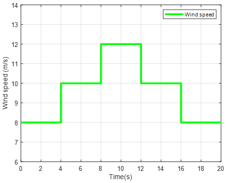
Figure 9. Wind speed profile in scenario 1
Figure 10. Tip speed ratio (TSR) of wind turbine
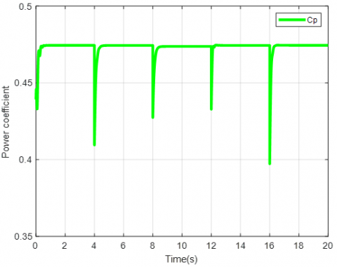
Figure 11. Power coefficient of PMSG
Figure 12. Wind turbine rotor speed tracking in scenario 1
In Figure 9, the green lines illustrate the variations in wind speed over time: From 0 to 4 seconds, the wind speed is steady at 8 m/s. Between 4 and 8 seconds, it rises to 12 m/s and maintains that level throughout. From 8 to 12 seconds, the wind speed drops back to 8 m/s. It then increases again to 12 m/s from 12 to 16 seconds. Finally, from 16 to 20 seconds, the wind speed decreases once more to 8 m/s.
Figure 12 shows how the wind turbine rotor speed changes over time relative to a reference speed. The blue line represents the actual rotational speed of the wind turbine rotor during the observation period. The red line represents the reference speed, which indicates the speed the wind turbine rotor should achieve to operate efficiently.
Figure 13. Wind turbine rotor speed tracking error in scenario 1
Figure 14. Wind turbine pitch angle
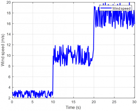
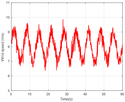
The next simulation scenario shown in Figure 15 indicates that a thunderstorm or a sudden change in weather may have occurred, causing a rapid increase in wind speed. The subsequent fluctuations indicate that the wind is unstable and may continue to change over time. Low wind speed: From 0 to about 10 seconds, the wind speed fluctuates between 4-6 m/s, indicating very weak winds. Sudden acceleration: From about 10 seconds, the wind speed suddenly increases to about 16 m/s, indicating a large change in wind conditions. Large fluctuations: After the increase phase, the wind speed remains at 16 m/s with small fluctuations, indicating a continuous change in wind conditions.
Figure 15. Wind speed profile in scenario 2
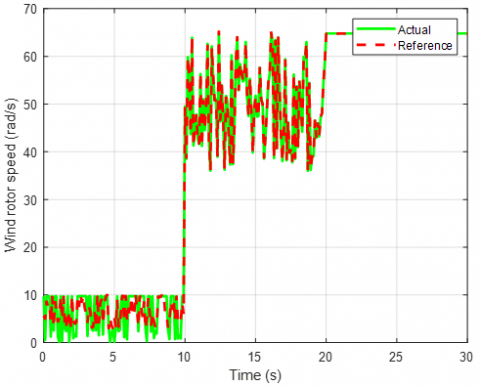
Figure 16. Wind turbine rotor speed tracking in scenario 2
Figure 17. Wind turbine rotor speed tracking error in scenario 2
In Figure 16, the blue line represents the actual rotational speed of the wind turbine rotor, oscillating around the reference line (shown as a red dashed line). This highlights the control error between the actual and target speeds. Figure 17 illustrates the system's performance in tracking the reference speed over time. The significant reduction in error after approximately 10 seconds shows the system’s capability to adapt and effectively maintain accuracy. The alignment between the actual speed and the reference speed reflects the ability to optimize the turbine’s performance amidst varying wind conditions (Figures 18).
Figure 18. Wind speed profile in scenario 3
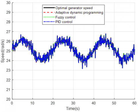
Figure 19. System response to controllers
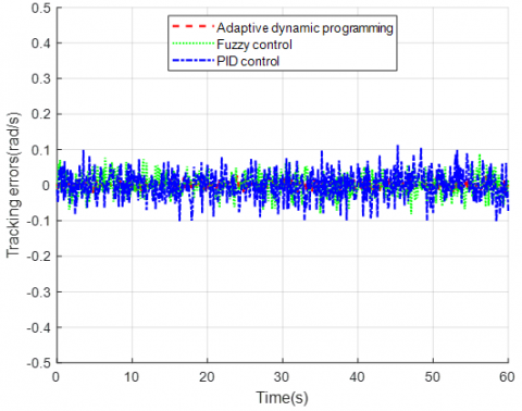
Figure 20. Tracking error of the system with the controllers
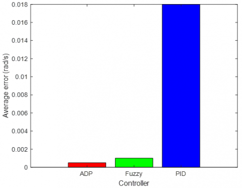
Figure 21. Average error of the controllers
Figure 19 shows the variation of the generator speed over a period of 60 seconds. The optimal speed (black line) shows the ideal speed that the generator should achieve. The ADP control method (red dashed line) shows a relatively good variation, close to the optimal speed with a small tracking error of approximately zero (Figures 20 and 21). The Fuzzy control (green dotted line) has relative stability, but still shows small fluctuations. The PID control (blue dotted line) shows high fluctuations and instability, which indicates that improvements are needed to improve efficiency.
In this study, we have introduced an adaptive optimal control methodology for a WECS. The control framework comprises two main elements: a state observer designed with a neural network and an adaptive optimal controller based on ADP. The parameters of both the controller and the estimator are updated using feedback from the Critic neural network, which operates according to an objective function aimed at minimizing input error. A key benefit of this control strategy is its reliance solely on output feedback, eliminating the need for knowledge of the system's dynamic model. We have established the stability of the control system and the convergence of the updated parameters using Lyapunov stability theory. Simulation results demonstrate that this adaptive optimal control approach enhances energy output, ensures stability, and facilitates a swift response to changing environmental conditions, ultimately improving the operational efficiency of contemporary wind energy systems. Looking ahead, the proposed algorithm could be implemented in practical application models for further testing and evaluation.
This study was supported by University of Economics - Technology for Industries (UNETI), Ha Noi – Viet Nam; Website: http://www.uneti.edu.vn/.
[1] Ofualagba, G., Ubeku, E.U. (2008). Wind energy conversion system- wind turbine modeling. In 2008 IEEE Power and Energy Society General Meeting - Conversion and Delivery of Electrical Energy in the 21st Century, Pittsburgh, PA, USA, pp. 1-8. https://doi.org/10.1109/PES.2008.4596699
[2] Gonzalez, L.G., Figueres, E., Garcera, G., Carranza, O. (2009). Modelling and control in Wind Energy Conversion Systems (WECS). In 2009 13th European Conference on Power Electronics and Applications, Barcelona, Spain, pp. 1-9.
[3] Errouissi, R., Al-Durra, A., Debouza, M. (2018). A novel design of PI current controller for PMSG-based wind turbine considering transient performance specifications and control saturation. IEEE Transactions on Industrial Electronics, 65(11): 8624-8634. https://doi.org/10.1109/TIE.2018.2814007
[4] Tripathi, S.M., Tiwari, A.N. (2020). Real-time evaluation of PMSG-based wind turbine control involving PI controller parameters tuned with explicit damping ratio specification. In 2020 International Conference on Electrical and Electronics Engineering (ICE3), Gorakhpur, India, pp. 559-564. https://doi.org/10.1109/ICE348803.2020.9122971
[5] Gong, J., Xie, R. (2016). Adaptive control of PMSG-based small wind turbines in Region II. In 2016 35th Chinese Control Conference (CCC), Chengdu, China, pp. 8518-8522. https://doi.org/10.1109/ChiCC.2016.7554717
[6] Mastromauro, R.A. (2022). Performance analysis of a wind turbine system with adaptive hysteresis band control. In 2022 IEEE 16th International Conference on Compatibility, Power Electronics, and Power Engineering (CPE-POWERENG), Birmingham, United Kingdom, pp. 1-6. https://doi.org/10.1109/CPE-POWERENG54966.2022.9880901
[7] Bratcu, A.I., Munteanu, I., Ceanga, E. (2008). Optimal control of wind energy conversion systems: From energy optimization to multi-purpose criteria - A short survey. In 2008 16th Mediterranean Conference on Control and Automation, Ajaccio, France, pp. 759-766. https://doi.org/10.1109/MED.2008.4602183
[8] Kim, M.-K. (2017). Optimal control and operation strategy for wind turbines contributing to grid primary frequency regulation. Applied Sciences, 7(9): 927. https://doi.org/10.3390/app7090927
[9] Tian, S., Liu, Y., Li, B., Chi, Y., Tian, X. (2024). An optimal operation strategy of wind farm for frequency regulation reserve considering wake effects. Energy, 304: 131975. https://doi.org/10.1016/j.energy.2024.130456
[10] Kamal, E., Bayart, M., Aitouche, A. (2011). Robust control of wind energy conversion systems. In 2011 International Conference on Communications, Computing and Control Applications (CCCA), Hammamet, Tunisia, pp. 1-6. https://doi.org/10.1109/CCCA.2011.6031221
[11] Tamilchelvan, P., Arounassalame, M. (2016). Robust control design for wind energy conversion system using Genetic Algorithm (GA) tuned Fractional order controller. In 2016 International Conference on Circuit, Power and Computing Technologies (ICCPCT), Nagercoil, India, pp. 1-6. https://doi.org/10.1109/ICCPCT.2016.7530381
[12] Benrabah, A., Khoucha, F., Benyamina, F., Raza, A., Benbouzid, M. (2021). Robust control of grid-interfaced wind energy conversion system based on active disturbance rejection control. In Artificial Intelligence and Renewables Towards an Energy Transition, Springer, Cham, pp. 71-83. https://doi.org/10.1007/978-3-030-63846-7_7
[13] Yang, B., Yu, T., Shu, H., Dong, J., Jiang, L. (2018). Robust sliding-mode control of wind energy conversion systems for optimal power extraction via nonlinear perturbation observers. Applied Energy, 210: 711-723. https://doi.org/10.1016/j.apenergy.2017.08.027
[14] Wang, Y., Zhang, Z., Garcia, C., Rodríguez, J., Kennel, R. (2020). Robust predictive control of grid-side power converters for PMSG wind turbine systems with stability analysis. In 2020 IEEE International Conference on Industrial Technology (ICIT), Buenos Aires, Argentina, pp. 763-768. https://doi.org/10.1109/ICIT45562.2020.9067307
[15] El Attafi, A., El Alami, H., Bossoufi, B., AlQahtani, D., Motahhir, S., Almalki, M.M., Alghamdi, T.A.H. (2024). Robust control of a wind energy conversion system: FPGA real-time implementation. Heliyon, 10(15): e35712. https://doi.org/10.1016/j.heliyon.2024.e35712
[16] Marmouh, S., Boutoubat, M., Mokrani, L. (2016). MPPT fuzzy logic controller of a wind energy conversion system based on a PMSG. In 2016 8th International Conference on Modelling, Identification and Control (ICMIC), Algiers, Algeria, pp. 296-302. https://doi.org/10.1109/ICMIC.2016.7804126
[17] Alarcón, F., Velásquez, I., Hunter, R., Pavez, B., Moncada, R. (2018). PID-Fuzzy control strategy for nonlinear systems applied to small wind turbines. In 2018 13th IEEE International Conference on Industry Applications (INDUSCON), Sao Paulo, Brazil, pp. 277-282. https://doi.org/10.1109/INDUSCON.2018.8627276
[18] Chatri, C., Ouassaid, M. (2018). Design of fuzzy control T-S for wind energy conversion system based PMSG using LMI approach. In 2018 IEEE 5th International Congress on Information Science and Technology (CiSt), Marrakech, Morocco, pp. 466-471. https://doi.org/10.1109/CIST.2018.8596515
[19] Maafa, A., Mellah, H., Benaouicha, K., Babes, B., Yahiou, A., Sahraoui, H. (2024). Fuzzy logic-based smart control of wind energy conversion system using cascaded doubly fed induction generator. Sustainability, 16(21): 9333. https://doi.org/10.3390/su16219333
[20] Tiwari, R., Ramesh Babu, N., Sanjeevikumar, P. (2018). Fuzzy logic-based pitch angle controller for PMSG-based wind energy conversion system. In Advances in Smart Grid and Renewable Energy, Springer, Singapore, pp. 283-294. https://doi.org/10.1007/978-981-10-4286-7_27
[21] Teferra, D.M., Ngoo, L.M.H., Nyakoe, G.N. (2022). A fuzzy controlled pitch angle in a permanent magnet synchronous generator type wind energy conversion system. In 2022 IEEE 21st Mediterranean Electrotechnical Conference (MELECON), Palermo, Italy, pp. 324-329. https://doi.org/10.1109/MELECON53508.2022.9843136
[22] Tomin, N., Kurbatsky, V., Guliyev, H. (2019). Intelligent control of a wind turbine based on reinforcement learning. In 2019 16th Conference on Electrical Machines, Drives and Power Systems (ELMA), Varna, Bulgaria, pp. 1-6. IEEE. https://doi.org/10.1109/ELMA.2019.8771645
[23] Kannikka, E., Kanwal, N. (2021). Control of overload safety in wind turbines through blade pitch control implementing artificial intelligence. In 2021 International Conference on Electrical, Computer and Energy Technologies (ICECET), Cape Town, South Africa, pp. 1-6. IEEE. https://doi.org/10.1109/ICECET52533.2021.9698633
[24] Zhang, J., Zhao, X., Wei, X. (2022). Reinforcement learning-based structural control of floating wind turbines. IEEE Transactions on Systems, Man, and Cybernetics: Systems, 52(3): 1603-1613. https://doi.org/10.1109/TSMC.2020.3032622
[25] Guo, W., Liu, F., He, D., Si, J., Harley, R., Mei, S. (2014). Reactive power control of DFIG wind farm using online supplementary learning controller based on approximate dynamic programming. In 2014 International Joint Conference on Neural Networks (IJCNN), Beijing, China, pp. 1453-1460. https://doi.org/10.1109/IJCNN.2014.6889871
[26] Yaramasu, V., Wu, B. (2017). Model Predictive Control of Wind Energy Conversion Systems. John Wiley & Sons. https://doi.org/10.1002/9781119082989
[27] Sarsembayev, B., Suleimenov, K., Mirzagalikova, B., Do, T.D. (2020). SDRE-based integral sliding mode control for wind energy conversion systems. IEEE Access, 8: 51100-51113. https://doi.org/10.1109/ACCESS.2020.2980239
[28] Liu, D., Wei, Q., Wang, D., Yang, X., Li, H. (2017). Adaptive Dynamic Programming with Applications in Optimal Control. Berlin: Springer International Publishing, pp. 45-47. https://doi.org/10.1007/978-3-319-50815-3