Anssam Yahya Kames*![]() | Ali Hussien Mary
| Ali Hussien Mary![]()
© 2025 The authors. This article is published by IIETA and is licensed under the CC BY 4.0 license (http://creativecommons.org/licenses/by/4.0/).
OPEN ACCESS
This paper proposed an Adaptive Cruise Control (ACC) control algorithm in vehicles. The ACC aims to determine required acceleration based on the distance measured between cars and the speed of the vehicle itself. The objective of this control system is to follow the front vehicle with a safety distance between lead and ego vehicles. For this purpose, the proposed controller is based on the PI controller applied to a ACC system. The proposed control system consists of two parts: an upper and lower controller. The upper controller decided which mode would be active: distance or speed control. The lower part controller is the PI controller, which determines the appropriate control signal. The Slap Swarm Algorithm (SSA) optimization algorithm has been used for tuning the parameters of the proposed controller. The simulation results of the proposed algorithm show that it provides excellent performance.
ACC, ADAS, optimal PID control, optimization algorithm, SSA
The focus on vehicle safety and driver assistance systems has expanded dramatically in recent years due to the rapid evolution of automotive technologies. The implementation of Advanced Driver Assistance Systems (ADAS) is important to enhance the safety of driving, mitigate human error, and optimize vehicle performance. To enhance driver comfort and safety, ADAS such as automatic emergency braking, adaptive cruise control, and lane keeping assist departure warning have become essential features of contemporary automobiles [1, 2]. The ability of Adaptive Cruise Control (ACC) to automatically adjust the vehicle's speed to stay a safe distance from other vehicles makes it stand out among these systems, improving driving convenience and safety on highways and congested routes [3, 4]. The primary purpose of ACC is to enable the car to stay at a pace that the driver has chosen while adapting to changing road conditions. This involves having the capacity to accelerate or decrease speed as necessary to maintain a safe gap from oncoming cars. The capacity of the ACC system to maintain a seamless transition between distance regulation and speed control is essential for enhancing driver comfort and safety [5]. To improve performance, ACC systems have been subjected to a variety of control techniques, the most popular of which is the Proportional-Integral-Derivative (PID) controller. PID controllers are useful for maintaining constant speeds or distances because they modify control inputs according to the proportional, integral, and derivative of the error between the desired and actual vehicle states [6, 7]. Nonetheless, the investigation of more sophisticated control techniques has been prompted by PID controllers' shortcomings in managing non-linear vehicle dynamics and shifting road circumstances [8]. Traditional PID controllers are designed for linear systems, while the vehicle dynamic is a nonlinear system, and its performance cannot be controlled by simple linear control methods. Model Predictive Control (MPC) is one such technique that maximizes control actions over a future time horizon by utilizing a predictive model of the vehicle's dynamics. This makes MPC a desirable alternative for ACC systems since it enables it to manage constraints more skillfully and adapt to changing traffic conditions [9]. Sliding Mode Control (SMC), known for its robustness, forces the system state to adhere to a predetermined surface, effectively managing disturbances and parameter variations. This method ensures that the ACC system can maintain performance under diverse and unpredictable road conditions [10]. Furthermore, fuzzy logic control (FLC), provides an alternative by addressing ambiguities and incomplete data, allowing for flexibility in handling intricate driving scenarios without necessitating an accurate mathematical model of the system [11, 12]. The capacity of neural network-based control techniques to learn from and adjust to intricate, non-linear vehicle dynamics has drawn attention in more recent times. Neural Network Control can boost the ACC system's reactivity to changing traffic patterns and its ability to maintain safe driving conditions by utilizing real-time traffic data [13, 14]. PID, MPC, FLC, SMC, and Neural Network Control are five control systems that each have advantages and disadvantages. The selection of a method is contingent upon the particular design requirements of the ACC system, which encompass elements like as robustness, flexibility, and performance under varying driving situations [15]. Current studies keep expanding the capabilities of ACC technology. In order to reconcile the predictability of MPC with the simplicity of PID, Chen et al. investigated a hybrid control approach that enhances vehicle stability and safety in dynamic traffic situations [16]. Similarly, Li et al. improved the system's capacity to handle uncertainties and adjust to real-time traffic fluctuations with a unique approach that combined fuzzy logic and neural networks [17]. Furthermore, Zhang et al. demonstrated the promise of artificial intelligence in upcoming autonomous driving applications by concentrating on deep learning techniques to enhance the adaptability and accuracy of ACC systems in urban driving conditions [18]. The suggested control method is important because it improves the efficiency of automobiles' ACC systems by responding quickly and precisely to variations in the speed and distance between cars. Compared to conventional techniques, the system provides greater stability and lowers tracking errors by using the Salp Swarm Algorithm (SSA) to adjust the controller's parameters. Additionally, by optimizing fuel usage, lowering the chance of accidents, and keeping a constant safe distance, the suggested control system increases efficiency. This study shows how to create novel solutions for intelligent vehicle control systems by fusing traditional control methods with cutting-edge optimization algorithms.
Economic and Environmental Analysis of the ACC System
The ACC system has significant economic and environmental considerations. Although the main objective of the ACC system is improving driving safety and comfort, it has many substantial economic benefits as well as environmental advantages. However, it must take into account the serval challenges and implementation cost. Optimizing the speed and manipulating the acceleration /braking system, can reduce the amount consumed fuel. Moreover, installing ACC with a vehicle may increase the sealing of these vehicles and also improve traffic flow. ACC can contribute to reducing CO2 emissions by using fuel effectively with saving fuel and it can support global and regional environmental goals.
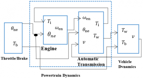
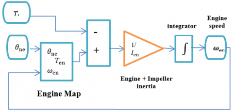
The longitudinal dynamics of the vehicle which is shown in Figure 1 is consists of two subsystems, The first one includes the engine, gearbox, and torque convertor while the second one related to external forces applied to the vehicle. In Figure 1(a) and (b), the model of the engine and torque converter are shown respectively and are represented by the following equations:
$I_{\mathrm{en}} \dot{\omega}_{\mathrm{en}}=T_{\mathrm{en}}\left(\theta_{\mathrm{ne}}, \omega_{\mathrm{en}}\right)-T_{\mathrm{i}}$ (1)
$T_{\mathrm{i}}=\left(\frac{\omega_{\mathrm{en}}}{k}\right)^2$ (2)
$T_{\mathrm{t}}=C_{\mathrm{t}} T_{\mathrm{i}}$ (3)
where, Ten denotes the torque of the engine, Ine represents the total moments of inertia, ωen refers to the speed of the engine, θne represents the angle of throttle and Ti known as torque convertor which is related to the engine speed and Turbine torque Tt, and k is the torque ratio while Ct denotes capacity factor.
The torque in the wheel can be determined as follows:
$T_{\mathrm{w}}=R_{\mathrm{g}} R_{\mathrm{fd}} T_{\mathrm{t}}$ (4)
where, Rg and Rfd in Eq. (4) refer to the gear ratio and drive ratio respectively.
(a)
(b)
Figure 1. (a) Vehicle longitudinal dynamics; (b) Engine dynamics
The forces of longitudinal that effect on the vehicle are: Force of traction (F), Force of aerodynamic (Faero), Rolling resistance force (Froll) and Gravitational force (Fgrav).
These forces can be expressed as follows:
$F=\frac{\left(T_{\mathrm{w}}+T_{\mathrm{b}}\right)}{r}$ (5)
$F_{\mathrm{aero}}=\frac{1}{2} C_{\mathrm{d}} A \rho v^2$ (6)
$F_{\text {roll }}=\mathrm{fmgcos}(\beta)$ (7)
$F_{\text {grav }}=\operatorname{mgsin}(\beta)$ (8)
where, Tw refers to the powertrain torque, Tb represents the torque produced by the braking system, r is the radius of the wheel, Cd represents the aerodynamic drag coefficient, A denotes the cross area of vehicle, ρ is the density of air, f denotes is the resistance coefficient of rolling, β refers to the grade of road, g is the acceleration of gravitational and m is the mass total of vehicle.
The dynamic model of the vehicle can be written based on Newton's second law as follows:
$\begin{aligned} m \dot{v}=F_x-F_{\text {aero }}- & F_{\text {roll }}-F_{\text {grav }} \Rightarrow m \dot{v} \\ & =F_x-\frac{1}{2} C_{\mathrm{d}} \mathrm{A} \rho v^2-f m g \cos (\beta) \\ & -m g \sin (\beta)\end{aligned}$ (9)
The SSA is an optimization method presented by Mirjalili and colleagues [19] to imitate the behavior of the Salp chain in searching about optimal food sources. SSA is unlike the Genetic algorithm which is suffering from high calculations such as mutation and crossover. SSA uses a simple mathematical model to update the position. With respect to the Ant Colony Optimization (ACO) algorithm, SSA is more general because ACO is designed at first for discrete problems while SSA is designed for continuous and discrete optimization problems. Moreover, SSA gives results with high accuracy for the Grey Wolf Optimizer (GWO). Finally, in comparison with Particle Swarm Optimization (PSO), SSA is more suitable for problems with high dimensional data or high nonlinearity. In this algorithm, the Salps are divided according to their positions in the chain into leaders and followers. The Salp chain, leader position, and follower position are expressed in the following:
$X_i=\left[\begin{array}{ccc}x_1^1 & . . & x_n^1 \\ \cdot & . . & \cdot \\ x_1^m & . . & x_n^m\end{array}\right]$ (10)
A group leader and followers must be chosen to mimic the salp swarm mechanism. The individual salp is considered the leader who takes charge of the entire squadron, while the other salps are considered followers. With each subsequent movement, the leader of this formation is responsible for directing the group toward a safer location. The mathematical translation of the leader of the swarm of slaps is shown in Eq. (11) where x is the two-dimensional location of each slap and y is the target food [19]:
$x_i^1=\left\{\begin{array}{l}y_i+r_1\left(u b_i-l b_i\right)+r_2+l b_i \\ y_i+r_1\left(u b_i-l b_i\right)+r_3+l b_i\end{array}\right.$ (11)
$x_i^1$ represents the leader position, $y_i$ represents the target food position in the $i^{\text {th }}$ dimension, $\mathrm{ub}_{\mathrm{i}}$ represents the upper bound of the $i^{\text {th }}$ dimension, $l b_i$ represents the lower bound of the $j^{\text {th }}$ dimension, and $r_1, r_2$, and $r_3$ are random numbers. Although SSA is a long series of salps, this kind of method can avoid local maximum or minimum solutions. By equating its progress towards the target meal, Eq. (12) depicts the leading salp's food perusing procedure. This is a critical factor in SSA that directs subordinate salps to capture food sources efficiently.
$r_1=2 e^{2 f / F}$ (12)
where, l/F is the ratio of the current iteration to the maximum number of salp swarm iterations that have been envisioned. Additionally, $r_2$, and $r_3$ are given random approximations between 0 and 1, which, depending on the step size, dictate the direction of the subsequent location of each $i^{\text {th}}$ dimension. Eq. (13) illustrates how Newton's equation of motion is used to determine the followers' following placements.
$x_i^j=\frac{1}{2} \gamma t^2+\gamma_0 t$ (13)
where, $j \geq 2$ and $\mathrm{x}_{\mathrm{i}}^{\mathrm{j}}$ represents the followers of the position. The $i^{\text {th }}$ dimension direction for every follower indicated by the superscript of $x$ is represented by the expression above. $t$ stands for time, and $\gamma_0$ is the salp follower's initial velocity, which is taken to be zero. Since the number iteration in the optimization analysis often represents time, the time variable was chosen to have a step size of one.
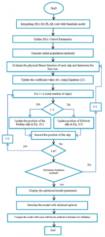
Figure 2. The flow chart of SSA
$\gamma=\frac{\gamma_{\mathrm{f}}}{\gamma_0}$ (14)
$\gamma_0=\frac{x-x_0}{t}$ (15)
Importantly keep in mind that the salp chain may move toward the ever-changing global optimum (food source) and use the allocated search area to find a finer answer. Several key features of SSA that distinguish it from traditional optimization techniques are as follows [19]:
1. The algorithm keeps the best result, after each iteration, and attributes it to the global optimal variable (food source). Thus, it will not be eliminated, even if the total population decreases.
2. The leading salp is constantly searching and exploiting the area around him in search of the best solution because the SSA simply updates the salp's position regarding the food supply, which is one of the best solutions so far.
3. To allow the salps strains to gradually approach the leading strains, SSA adjusts their relative positions.
4. The salp follower movements keep the SSA from crashing quickly into the local optimum;
5. We can explore the algorithmic search space at the beginning and exploit it at the end of the iteration process thanks to the adaptive decrement of the parameter r1.
6. The SSA only has one primary regulating parameter (r1), which simplifies and makes implementation simple.
The SSA's ability to handle optimization issues more effectively than traditional optimization techniques stems from the aforementioned advantages, which served as the impetus for the current study. Additionally, by consistently avoiding becoming stuck in local solutions, this adaptive algorithm enables SSA to find an accurate evaluation of the optimal solution. In Figure 2, the flow chart shows the performance of SSA in terms of optimizing the PID controller parameters of an ACC system.
The SSA randomly deploys all search agents (salps) around the specified search space. It then evaluates the current salp set to determine the leader and forces others to follow. Eq. (12) is used in this step to update the variable r1. Eq. (11) provides the SSA with information about the leader's condition, and Eq. (13) adjusts the follower salps' location correspondingly. To improve the quality of the salps as much as feasible, all steps—aside from the initialization phase will be repeated until the stopping condition is satisfied.
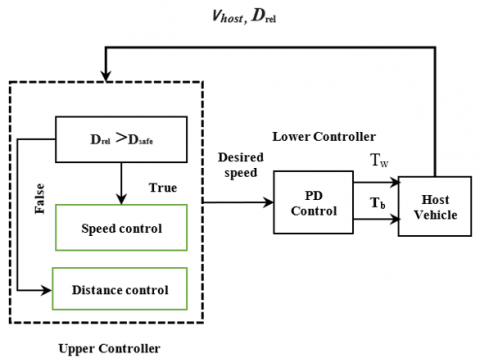
The proposed controller consists of two sub controllers upper and lower sub controllers as shown in Figure 3. The upper controller which can be called adaptive cruise controller determine the desired speed and desired distance based on the relative distance between the host and leading vehicles and the speeds of the host and leading vehicles. The lower level controller attempts to track the leading vehicle with safety distance between vehicles.
Figure 3. Proposed control
4.1 Adaptive cruise controller
This controller regulates the speed of the host vehicle and the leading vehicles according to the distance between them. This controller algorithm of operates as follows:
1) If the distance between vehicle is greater than safety distance, the vehicle will be accelerated to the desired speed
2) If the distance between the two vehicles in the acceptable range of safety distance, the vehicle will be decelerated to the desired speed.
4.2 Adaptive cruise control algorithm
The inputs for the proposed adaptive cruise control algorithm are: Relative distance, and host vehicle and the output is: desired acceleration.
$D_{r e l}=D_o+v t$ (16)
Do default spacing
Dsafe set by the designer
If
$D_{\text {rel }}>D_{\text {safe }}$ (17)
Then accelerate vehicle according to the velocity set by the driver.
If
$D_{\text {rel }}<D_{\text {safe }}$ (18)
Then deaccelerate vehicle according to the velocity lead vehicle.
This controller will decide which control mode will be applied speed control (acceleration) or distance control (deceleration). The output of this controller will be input to the 2nd part of the proposed controller (lower level).
4.3 PD controller tuning with multi objective function
A PD controller has been used as a low-level controller to determine the required values for braking pressure and throttle angle. When the relative distance is less than safe distance the mode of control is distance control and the proposed control law used is:
$\mathrm{u}_{\text {speed }}=\mathrm{k}_{\mathrm{p}} \mathrm{D}_{\mathrm{err}}+\mathrm{k}_{\mathrm{d}} \frac{\mathrm{dD}_{\mathrm{err}}}{\mathrm{dt}}$ (19)
kp propositional gain
kd derivative gain
When the safe distance is less than the relative distance, the speed control is the control mode and the proposed control law used is:
$u_{\text {dis }}=\min \left(u_{\text {speed }}, k v_{\text {err }}\right)$ (20)
where,
$v_{\text {err }}=v_{\text {set }}-v$ (21)
$k v_{e r r}$ is proportional gain.
Due to importance of using optimization algorithm to tune the parameters of controllers [20], the following objective function used to tune the gain of the proposed controller.
$o b j=\int_0^{t_f}\left(w_1\left(d_{r e l}-d_{s a f}\right)^2+w_2\left(v-v_{s e t}\right)^2\right) d t$ (22)
In this part, the performance of the longitudinal dynamics of autonomous vehicles proposed control is discussed. Three cases are presented, in the first case; proposed Adaptive cruise system checked without disturbance; while in the second case; a pulse disturbance applied that change the acceleration of vehicle suddenly; in the last case a disturbance signal applied to change the required the softy distance. Table 1 lists the values of the dynamic parameters of the vehicle used in the simulation.
Table 1. Dynamic model parameters [21]
|
Parameter |
Value |
|
mo |
1250 kg |
|
r |
0.29 m |
|
Kb |
540 Nm/mPa |
|
Iei |
0.16 kg·m2 |
|
Cd |
0.800 N/V |
|
f |
0.318 N/V |
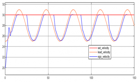
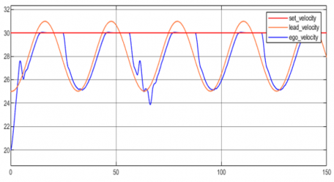
Figure 4. Velocities in Case 1
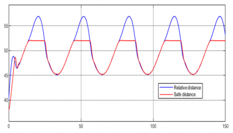
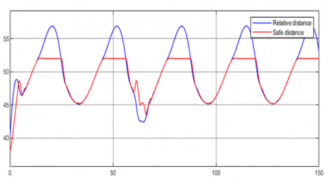
Figure 5. Distance in Case 1
Case 1: The host and lead vehicles started with initial speeds 28 m/s and 36 m/s while the initial distance between vehicles is 8 m. When ACC system is active, the host vehicle tracks the lead vehicle instead of driver set velocity.
When the required value of the distance between vehicles is reached, the control mode in ACC convert to distance control and the proposed controller in ACC system follows the lead vehicle with the same speed in order to keep the safe distance between vehicles as shown in Figure 4 and Figure 5 respectively.
The proposed controller still operates in distance control when the driver set speed is greater than speed of lead vehicle. It can be notice from fig, that the distance between host and lead vehicle reach the desired distance with host vehicle speed converges to the desired velocity set be the ACC system which equal to the deriver set velocity in speed control mode and lead vehicle speed in speed control while the desired velocity in distance control mode is equal to velocity of lead vehicle.
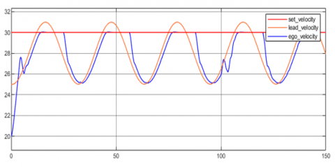
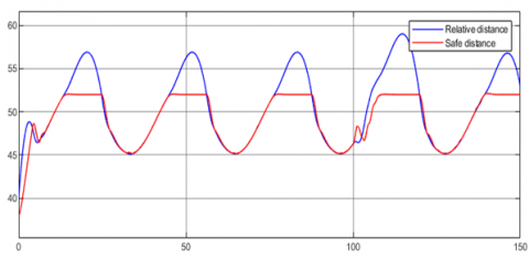
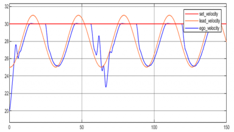
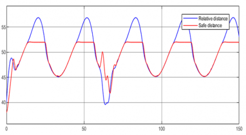
Case 2: To check the performance of the proposed controller during a disturbance, at time t=100 sec, a pulse signal with amplitude equal to applied to change the acceleration. The velocities of vehicles and distance between vehicles are shown in Figures 6 and 7 respectively. It can be noticed the changes occur after 100 seconds and ability of the proposed controller to retain to tracking the lead vehicle with short time.
Case 3: In this test, safety distance between vehicles changed suddenly at time t=60 second and increased the safety distance by 3 meter and then by 5 meters. The proposed controller shows its performance due to an increase of 3 meters in Figures 8 and 9 while Figures 10 and 11 show the proposed controller's performance due to an increase of 5 meters. From these figures, it can be noted that when the distance becomes less than the safe distance between vehicles, the controller tries to increase the distance with the lead vehicle, thus the velocity of the host vehicle decreased to increase the distance with the lead vehicle. When we review these results, we can see how strong the proposed controller is in facing external disturbances.
Figure 6. Velocities in Case 2
Figure 7. Distance in Case 2
Figure 8. Velocities in Case 3
Figure 9. Distance in Case 3
Figure 10. Velocities due to large disturbance in Case 3
Figure 11. Distance due to large disturbance in Case 3
This paper presented an optimal control method for vehicle ACC systems to produce a safety distance between vehicles with speed tracking. The proposed controller consists of two parts upper and lower controllers. The upper controller decides the desired speed and selects control mode either control speed mode or control distance mode. The lower controller, determines the appropriate control signal required for the drivetrain torque, and braking torque by using a PD controller. The SSA optimization algorithm has been used to tune the gains of the PD controller taking into account the safety distance with another vehicle and tracking speed in the design objective function. Simulation results indicate a good performance for the proposed controller. It can improve the proposed controller by using a robust controller like SMC and it can use neural network to estimate the parameters of the vehicle dynamic.
[1] Kukkala, V.K., Tunnell, J., Pasricha, S., Bradley, T. (2018). Advanced driver-assistance systems: A path toward autonomous vehicles. IEEE Consumer Electronics Magazine, 7(5): 18-25. https://doi.org/10.1109/MCE.2018.2828440
[2] Li, X.R., Lin, K.Y., Meng, M., Li, X.X., Li, L., Hong, Y.G., Chen, J. (2021). Composition and application of current advanced driving assistance system: A review. arXiv preprint arXiv:2105.12348. https://doi.org/10.48550/arXiv.2105.12348
[3] Miyata, S., Nakagami, T., Kobayashi, S., Izumi, T., Naito, H., Yanou, A., Nakamura, H., Takehara, S. (2010). Improvement of adaptive cruise control performance. EURASIP Journal on Advances in Signal Processing, 2010: 295016. https://doi.org/10.1155/2010/295016
[4] Zhu, Z.X., Bei, S.Y., Li, B., Liu, G.S., Tang, H.R., Zhu, Y.H., Gao, C.C. (2023). Research on robust control of intelligent vehicle adaptive cruise. World Electric Vehicle Journal, 14(10): 268. https://doi.org/10.3390/wevj14100268
[5] Ali, F.M., Abbas, N.H. (2024). Adaptive cruise control system: A literature survey. Journal of Engineering, 30(9): 239-272. https://doi.org/10.31026/j.eng.2024.09.12
[6] Chaturvedi, S., Kumar, N. (2023). Design and implementation of an optimized PID controller for the adaptive cruise control system. IETE Journal of Research, 69(10): 7084-7091. https://doi.org/10.1080/03772063.2021.2012282
[7] Memon, Z.A., Unar, M.A., Pathan, D.M. (2016). Parametric study of nonlinear adaptive cruise control for a road vehicle model by MPC. arXiv preprint arXiv:1604.00556. https://doi.org/10.48550/arXiv.1604.00556
[8] Kabasakal, B., Üçüncü, M. (2022). The design and simulation of adaptive cruise control system. International Journal of Automotive Science and Technology, 6(3): 242-256. https://doi.org/10.30939/ijastech.1038371
[9] Al-Gabalawy, M., Hosny, N.S., Aborisha, A.H.S. (2021). Model predictive control for a basic adaptive cruise control. International Journal of Dynamics and Control, 9: 1132-1143. https://doi.org/10.1007/s40435-020-00732-w
[10] Boukattaya, M., Gassara, H., Damak, T. (2020). A global time-varying sliding-mode control for the tracking problem of uncertain dynamical systems. ISA Transactions, 97: 155-170. https://doi.org/10.1016/j.isatra.2019.07.003
[11] Mary, A.H., Miry, A.H., Miry, M.H. (2022). ANFIS based reinforcement learning strategy for control a nonlinear coupled tanks system. Journal of Electrical Engineering & Technology, 17: 1921-1929. https://doi.org/10.1007/s42835-021-00753-1
[12] Naranjo, J.E., Sotelo, M.A., Gonzalez, C., Garcia, R., De Pedro, T. (2007). Using fuzzy logic in automated vehicle control. IEEE Intelligent Systems, 22(1): 36-45. https://doi.org/10.1109/MIS.2007.18
[13] Mahadika, P., Subiantoro, A., Kusumoputro, B. (2020). Neural network predictive control approach design for adaptive cruise control. International Journal of Technology, 11(7): 1451-1462. https://doi.org/10.14716/ijtech.v11i7.4592
[14] Wang, Y., Guo, Z., Wu, J., Fu, S. (2022). Research on vehicle adaptive cruise control based on BP neural network working condition recognition. The Journal of Engineering, 2022(2): 132-147. https://doi.org/10.1049/tje2.12094
[15] Jain, Y.M. (2020). Comparison of model-predictive control and PID control for adaptive cruise control of UW EcoCAR vehicle. University of Washington.
[16] Peng, Y.C., Liu, D.Y., Wu, S.B., Yang, X.X., Wang, Y.S., Zou, Y.J. (2025). Enhancing mixed traffic flow with platoon control and lane management for connected and autonomous vehicles. Sensors, 25(3): 644. https://doi.org/10.3390/s25030644
[17] Alzaydi, A., Abedalrhman, K., Alotaibi, I., Alessa, F. (2024). Advancing autonomous vehicle navigation through hybrid fuzzy-neural network training systems. SSRN 5048252. https://doi.org/10.2139/ssrn.5048252
[18] Zhao, R., Wang, K., Che, W.B., Li, Y., Fan, Y.Z., Gao, F. (2024). Adaptive cruise control based on safe deep reinforcement learning. Sensors, 24(8): 2657. https://doi.org/10.3390/s24082657
[19] Mirjalili, S., Gandomi, A.H., Mirjalili, S.Z., Saremi, S., Faris, H., Mirjalili, S.M. (2017). Salp Swarm Algorithm: A bio-inspired optimizer for engineering design problems. Advances in Engineering Software, 114: 163-191. https://doi.org/10.1016/j.advengsoft.2017.07.002
[20] Miry, A.H., Mary, A.H., Miry, M.H. (2019). Improving of maximum power point tracking for photovoltaic systems based on swarm optimization techniques. IOP Conference Series: Materials Science and Engineering, 518(4): 042003. https://doi.org/10.1088/1757-899X/518/4/042003
[21] Marzbanrad, J., Tahbaz-zadeh Moghaddam, I. (2016). Self-tuning control algorithm design for vehicle adaptive cruise control system through real-time estimation of vehicle parameters and road grade. Vehicle System Dynamics, 54(9): 1291-1316. https://doi.org/10.1080/00423114.2016.1199886