Nitin K. Mishra![]() | Prerna Jain*
| Prerna Jain*![]() | Ranu
| Ranu![]() | Aishwarya Tiwari
| Aishwarya Tiwari
© 2024 The authors. This article is published by IIETA and is licensed under the CC BY 4.0 license (http://creativecommons.org/licenses/by/4.0/).
OPEN ACCESS
Due to tougher carbon restrictions and regulations, businesses have been researching approaches to decrease the amount of carbon emissions throughout the inventory supply process and achieve sustainable development. The two most common approaches are (i) decentralized, which involves implementing a carbon tax or cost for emitting carbon, and (ii) centralized, which includes introducing an emissions trading (cap-and-trade) mechanism. Within this research, we optimize a two-stage supply management system under FPH(finite planning horizon) while taking into consideration these two policies. Using a linear time and inventory-dependent demand model, we investigated various techniques within a specific time frame. We created and solved two distinct MINLP (Mixed Integer Non-Linear Programming) approaches for each carbon strategy. These models can assist businesses/firms in determining the minimum overall cost, optimal order quantity, optimal replenishment time, and replenishment cycles. Using mathematical tools, our sensitivity evaluations indicate that organizations can reduce overall projected emissions and costs by making parameter variations under both carbon regimes. We additionally showed that while both approaches optimize the overall supply chain cost, the order quantity and total emissions remain constant.
decentralized and centralized, linear demand time and inventory sensitive, finite planning horizon, carbon tax, and emissions trading schemes
Inventory management stands as a cornerstone of efficient supply chain operations, orchestrating the seamless flow of goods from procurement to distribution. Kumar et al. [1] emphasized its broad spectrum of activities, spanning procurement, storage, distribution, and replenishment, all aimed at maintaining optimal inventory levels. The significance of effective inventory management lies in its ability to strike a delicate balance between meeting customer demands and controlling costs.
Nagaraju et al. [2] underscored the central principle of ensuring the availability of the right inventory, at the right time, in the right place, and at the right cost. This principle is further accentuated by the pivotal role inventory plays as a substantial business asset, influencing financial resources and operational liquidity [3]. Moreover, efficient inventory management not only fulfills customer expectations but also aligns with broader organizational goals of sustainability and profitability, through cost control and waste reduction measures.
However, the traditional paradigm of inventory management faces new challenges in an era marked by heightened environmental consciousness and regulatory scrutiny. The emergence of carbon policies, aimed at curbing greenhouse gas emissions and promoting environmental sustainability, introduces a layer of complexity to inventory management strategies. In this context, the integration of carbon policies into inventory management practices becomes not only a regulatory necessity but also a strategic imperative for businesses aiming to reconcile operational efficiency with environmental responsibility.
Human-caused emissions, notably carbon dioxide, are responsible for global warming, which poses a serious threat to the climate and the existence of humanity. To address this issue, regulatory bodies and policymakers throughout the world have established carbon regulations targeted at preventing pollution. Carbon policies can be listed into different kinds: carbon tax/cost legislation, carbon cap-and-trade regulation, and other policies [4].
Under the carbon tax program, every unit of carbon dioxide emitted is subject to a penalty. This program is a fee imposed by regulatory agencies or decision-makers on firms for their carbon emissions during their processes. However, businesses and organizations can keep releasing carbon dioxide as needed, they are required to pay charges for each unit of carbon emitted [5].
Decision-makers enforce the carbon cap [6] framework under the Carbon Cap-and-Trade regime. The government or decision-makers set a carbon cap or limit and allow firms to buy or sell carbon credits under this policy. Whenever a company generates less carbon than the limit, it can sell its leftover carbon credits to other businesses and organizations. If a corporation or organization exceeds its carbon emission quota, it can buy carbon credits from other organizations that release less carbon. Carbon cap policies impose a ceiling on the number of carbon emissions that enterprises or organizations can produce, and exceeding this quota results in a hefty penalty [7-9].
Carbon taxation and emissions trading schemes are two important regulatory Systems used by many governments worldwide. Many European regions participate in the European Union Emissions Trading Systems (EU-ETS), the world's most extensive program to buy greenhouse emissions (GHG) [10]. Some nations, however, have either enacted or are in the process of implementing their carbon price or cap-and-trade legislation.
Although supply chains are a main priority for several firms, especially multinational organizations, and groups such as Walmart, there is a concentrated push to eliminate pollution across inventory supply networks. Because this sector contributes significantly to emissions, researchers and industry experts place high importance on inventory replenishment models that can lower both costs and emissions. In response to this need, we have developed a model aimed at optimizing costs and examining supply chains under two distinct scenarios: a decentralized supply chain implementing a carbon tax program, and a centralized supply chain operating under an emission carbon cap and trade system, all within a finite planning horizon.
This paper systematically explores inventory management within carbon regulations and sustainability. We begin with a literature review in Section 2, identifying gaps and setting research goals. In Section 3, we establish assumptions and notations, leading to the presentation of our mathematical model in Section 4. Here, both centralized and decentralized approaches are analyzed. Section 5 demonstrates practical application through a numerical example, providing insights for industry. Section 6 conducts sensitivity analysis, ensuring robustness and managerial insights. Employing "Wolfram Mathematica 13.0," our methodology enhances accuracy. In Section 7, we summarize findings, propose future research directions, and reflect on our contributions to inventory management and sustainability.
Inventory management is all about keeping track of supplies and making sure they're in the right place at the right time. But nowadays, with carbon rules in place, things have gotten a bit more complicated. In this section, we'll look at what researchers have been saying about managing inventory under these new carbon regulations.
Kung et al. [8] have delved into the collaborative efforts between manufacturers and retailers to reduce their carbon footprint. Their study aimed to understand how a carbon tax influences these joint actions within the supply network, and its broader impacts on the economy and environmental sustainability. They found that businesses working together can make a significant difference in reducing carbon emissions, especially when guided by carbon policies.
Other studies [9, 10] have focused on the nitty-gritty of managing inventory in the face of additional costs due to carbon emissions. Their research developed various inventory management systems designed to cope with these extra expenses imposed by carbon policies. By implementing strategies like carbon cost policies and gradual emission tax policies, businesses can navigate through these challenges while maintaining efficient supply chains.
Cheng et al. [11] explored how different types of supply chains-like traditional retail versus digital-adapt to carbon regulations. They investigated the implications of carbon cap regulations on both centralized and decentralized supply chain channels. By analyzing various scenarios, they aimed to understand how these regulations impact the management and flow of goods in different supply chain contexts.
The studies [12, 13] delved into innovative strategies for reducing emissions while managing inventory effectively. They experimented with approaches such as cap-and-trade initiatives and carbon offset strategies to find optimal production and inventory policies. By exploring a range of emission reduction strategies, these studies shed light on practical solutions for businesses striving to balance cost-effectiveness with environmental responsibility.
The studies [14, 15] focused on optimizing inventory management practices to align with sustainability goals. They developed mathematical models to assess the impact of carbon policies, including carbon taxes and cap-and-trade regimes, on supply chain operations. By integrating environmental considerations into inventory management decisions, these studies highlighted pathways for businesses to achieve both economic and environmental objectives.
Lastly, Hua et al. [16] examined the financial implications of carbon regulations on trade credit-a crucial aspect of business transactions. Their study investigated how carbon constraints influence optimal trade credit preferences under different policy scenarios. By understanding the financial dynamics shaped by carbon rules, businesses can adapt their financial strategies to mitigate risks and capitalize on opportunities in a carbon-constrained environment.
As we reflect on the breadth of research in this area, it's evident that managing inventory under carbon regulations poses multifaceted challenges and opportunities for businesses. The main findings of these researchers are summarized in Table 1, highlighting key insights into how various carbon policies impact inventory management practices. In the subsequent sections, we'll delve deeper into the gaps identified in the existing literature and outline the research objectives aimed at addressing these gaps comprehensively.
Based on the study of the literature, it is possible to conclude that in recent decades, many researchers have included different carbon policies in enhancing the inventory replenishment model. Nevertheless, many researchers have concentrated on a single carbon policy, with just a few quantitative articles considering many policies at the same time. Additionally, research investigating various carbon policies has mainly focused on deterministic demand. Until now, no analysis has evaluated several carbon policies concurrently under a finite scheduling horizon for uneven replenishment cycle length. Demand is influenced by both time and inventory levels.
The lack of research on inventory modeling that examines demand that is influenced by both time and inventory levels in the context of two significant carbon regulations over a finite planning horizon is examined in this research study. Earlier literature has not investigated these policies under an FPH, making this study the first to present such approaches. As a result, the research aims to cover a gap by providing a novel approach to gain new insights.
Table 1. Comparison of literature review
|
Study |
Linear Demand Time & Inventory Sensitive |
Finite Planning Horizon |
Carbon Tax Policy |
Carbon Cap and Trade |
|
[11] |
Yes |
Yes |
Influences collaborative efforts, economy, and environmental efficiency |
- |
|
[12] |
- |
- |
Managed by a carbon cost policy |
- |
|
[13] |
- |
- |
Gradual carbon tax policy |
- |
|
[5] |
Yes |
Yes |
Considered in a deterministic multiperiod production planning framework |
- |
|
[14] |
- |
- |
- |
Considered under a carbon cap policy |
|
[15] |
- |
- |
- |
Considered under a carbon cap-and-trade mechanism |
|
[7] |
- |
- |
Various carbon policies can achieve cost and emissions reduction goals. |
- |
|
[16] |
- |
- |
Considered both carbon taxes and carbon cap-and-trade regimes. |
- |
|
[17] |
- |
- |
- |
Evaluated trade credit under carbon regulations |
|
[18] |
Yes |
Yes |
Considered all three carbon policies (tax, cap-and-trade, cap-and-offset) |
- |
|
[19] |
- |
- |
Evaluated carbon tax and cap-and-trade policies |
Considered centralized and decentralized supply networks |
|
This Study |
Yes |
Yes |
Yes |
Yes |
3.1 Notations
|
a |
The annual beginning demand rate during the initial phase of the inventory management cycle. |
|
b |
Over a year, the customer demand rate increases as well. |
|
θ |
The rate of demand is determined by the level of inventory. |
|
Hr |
The cost of holding a particular thing in rupees per unit per year. |
|
Ss |
The total cost is estimated in dollars per order and incorporates both the setup and shipment costs. |
|
Cp |
The cost of purchasing a single unit is given in dollars per unit. |
|
Ij+1(t) |
The level of stock from ti to ti+1 during the (i+1)th cycle, where ti is the cycle's beginning time where $t_i \leq t \leq t_{i+1}$. |
|
Qj+1 |
which symbolises the number of items ordered within the (i)th cycle at the time t and t is any period that lie in between ti and ti+1. |
|
$P_r$ |
For wholesale trades, the price per unit is in rupees. |
|
Or |
The ordering cost per transaction during the beginning of the managing inventory period. |
|
$\hat{c}$ |
The emissions amount generated per order. |
|
$\hat{P}_r$ |
The CO2 emissions quantity connected with each purchasing unit. |
|
$\widehat{h_r}$ |
The quantity of greenhouse gas emissions generated per unit of time while maintaining stock. |
3.2 Assumptions
(1) The planning horizon is assumed to be limited or finite in this framework.
(2) This model does not assume or predict the existence of deficits or shortages in demand.
(3) This model presupposes that orders will be finalized promptly as they are placed, which implies a waiting time is zero.
(4) In this model, the cost of holding inventory within the supply process is assumed to be I per unit of time.
(5) In this model, demand for goods is linearly related to time, meaning an increasing rise in demand throughout the planning horizon.
An inventory supply network with a solo supplier and a solo retailer is regarded to involve a single product or item in this model.
The formulation of carbon emissions is essential for accurately quantifying the environmental impact of the activities under investigation. We have carefully selected specific terms and defined parameters to ensure the robustness and relevance of our carbon emissions model. The terms included in the carbon emissions formulation are derived from established models and equations widely recognized in the field of environmental science and sustainability. These terms reflect various factors influencing carbon emissions, such as production processes, transportation methods, and energy consumption.
Furthermore, the parameters defining these terms are chosen to capture the essential aspects of the system under study. We have based our parameter definitions on empirical data, theoretical models, and industry standards to ensure accuracy and reliability. Specifically, the parameters are sourced from authoritative literature, including works [6, 20], among others, which provide valuable insights into carbon emissions estimation methodologies.
The shifts in the quantity of stock $I_{n_{(i+1)}}(t)$ over time can be derived from the solution to the given mathematically differential Eq. (1) below, which corresponds to the (i+1)th replenishment cycle:
$I_{n_{(i+1)}}(t)=e^{-\theta t} \int_t^{t_{i+1}}(a+b u) e^{\theta * u} \mathrm{dt}$ (1)
where, $t_i<\mathrm{t}<t_{i+1}$
$\begin{gathered}I_{n_{(i+1)}}(t)=0 \\ Q_{i+1}=I_{i+1}\left(t_i\right)=\int_{t_{i+1}}^{t_i}(a+b u) e^{\theta *(u-t)} \mathrm{dt} \\ I_{n(i+1)}(t)=\int_t^{t_{i+1}}(a+b u) e^{\theta(u-t)} \mathrm{du}\end{gathered}$ (2)
$\begin{aligned} & I_{n_{(i+1)}}(t)=\left[\frac{(a+b u) e^{\theta(u-t)}}{\theta}-\frac{b}{\theta^2} e^{\theta(u-t)}\right]_t^{t_{i+1}} \\ & I_{n_{(i+1)}}(t)=\frac{\left(a+b t_{i+1}\right) e^{\theta\left(t_{i+1}-t\right)}}{\theta}-\frac{b}{\theta^2} e^{\theta\left(t_{i+1}-t\right)} \frac{(a+b t)}{\theta}+\frac{b}{\theta^2}\end{aligned}$
The order quantity for ith cycles
$\begin{gathered}Q_{i+1}=I_{i+1}\left(t_i\right)=\int_{t_i}^{t_{i+1}}(a+b t) e^{\theta\left(t-t_i\right)} \mathrm{dt} \\ Q_{i+1}=I_{i+1}\left(t_i\right)=\left[\frac{(a+b u) e^{\theta\left(u-t_i\right)}}{\theta}-\frac{b}{\theta^2} e^{\theta\left(u-t_i\right)}\right]_{t_i}^{t_{i+1}}\end{gathered}$
$\begin{gathered}Q_{i+1}=I_{i+1}\left(t_i\right)=\frac{\left(a+b t_{i+1}\right) e^{\theta\left(t_{i+1}-t_i\right)}}{\theta}- \frac{b}{\theta^2} e^{\theta\left(t_{i+1}-t_i\right)}-\frac{\left(a+b t_i\right)}{\theta}+\frac{b}{\theta^2}\end{gathered}$ (3)
According to the studies [6, 9], the proposed study includes the $\hat{c}$ fixed quantity emission, $\hat{P}$ connected with inventory replenishment, and $\widehat{h_r}$ associated with inventory holding or management (refrigeration effect).
$A m t_{\text {carbon }}=\hat{c}+\hat{P}_r * Q_{i+1}+\widehat{h_r} \int_{t_i}^{t_{i+1}} \int_t^{t_{i+1}}(a+b u) e^{\theta(u-t)} d u \, d t$
4.1 Decentralized case
In decentralized decision-making within the supply chain, each entity, including suppliers, manufacturers, and distributors, operates autonomously, making decisions independently without coordination. This lack of coordination means that each party pursues its own interests and objectives without considering the broader implications for the entire supply chain. Consequently, the total cost incurred in the decentralized supply chain encompasses several components, including ordering cost, holding cost, purchasing cost, and the cost of carbon tax.
$\begin{gathered}\mathrm{Tc}_{\mathrm{Ret}}\left(n_1, t_i\right)=n_1 * O_r+H_r \sum_{i=0}^{n_1} \int_{t_i}^{t_{i+1}} I_{n_{(i+1)}}(t) \mathrm{dt}+ P_r \sum_{i=1}^{n_1} Q_{i+1}+\sum_{i=0}^{n_m} \tau\left(\hat{c}+\hat{P}_r *\right. \left.Q_{i+1}+\hat{h}_r \int_{t_i}^{t_{i+1}} I_{n(i+1)}(t) \mathrm{dt}\right)\end{gathered}$ (4)
$\begin{gathered}T c_{R e t}\left(n_1, t_i\right)=n_1 * O_r+H_r \sum_{i=1}^{n_1} \int_{t_i}^{t_{i+1}} \int_t^{t_{i+1}}(a+ \\ b u) e^{\theta(u-t)} \mathrm{du} d t+P_r \sum_{i=1}^{n_1} \int_{t_i}^{t_{i+1}}(a+b t) e^{\theta\left(t-t_i\right)} \mathrm{dt}+ \\ \sum_{i=0}^{n_1-1} \tau\left(\hat{c}+\hat{P}_r * \int_{t_i}^{t_{i+1}}(a+b t) e^{\theta\left(t-t_i\right)} \mathrm{dt}+\widehat{h_r} \int_{t_i}^{t_{i+1}} \int_t^{t_{i+1}}(a+\right. \left.b u) e^{\theta(u-t)} du \,\, dt\right)\end{gathered}$
$\begin{gathered}T c_{\text {Ret }}\left(n_1, t_i\right)=n_1 * O_r+\left(H_r+\tau * \widehat{h_r}\right) \sum_{i=1}^{n_1} \int_{t_i}^{t_{i+1}} \int_t^{t_{i+1}}(a+ \\ b u) e^{\theta(u-t)} \mathrm{du}\, d t+\tau * \hat{c}+\sum_{i=0}^{n_1-1}\left(\left(P_r+\hat{P}_r * \tau\right) \int_{t_i}^{t_{i+1}}(a+\right. \\ \left.b t) e^{\theta\left(t-t_i\right)} \mathrm{dt}\right)\end{gathered}$
$\begin{gathered}T c_{R e t}\left(n_1, t_i\right)=n_1 * O_r+\tau * \hat{c}+\left(\frac{H_r+\tau * h_r}{\theta}+\left(P_r+\widehat{P}_r *\right.\right. \\ \tau) \sum_{i=1}^{n_1} \int_{t_i}^{t_i}(a+\mathrm{bt}) e^{\theta\left(t-t_i\right)} \mathrm{dt}-\frac{H_r+\tau * \hat{h}_r}{\theta}\left(a * H+\frac{1}{2} * b^* H^2\right)\end{gathered}$ (5)
where, $\mathrm{H}=t_{n_1}=t_{i+1}-t_i$
$T c_{\text {Sup }}\left(n_1, t_i\right)=n_1^* * S_r+\sum_{i=0}^{n^*-1} C_p * Q_{i+1}^*$ (6)
$T c_{S u p}\left(n_1, t_i\right)=n_1{ }^* * S_r+C_p \sum_{i=0}^{n_1{ }^*-1} \int_{t_i}^{t_{i+1}}(a+\mathrm{bt}) e^{\theta\left(t-t_i\right)} \mathrm{dt}$
$Q_{i+1}=\sum_{i=0}^{Q_{i+1}}=\sum_{i=0}^{n_1^*-1} Q_{i+1}^{n_1-1}(a+b t) e^{\theta\left(t-t_i\right)} \mathrm{dt}$ (7)
$\begin{gathered}T c_{\text {System }}\left(n_1, t_i\right)=n_1 *\left(O_r+S_r\right)+\tau * \hat{c}+ \\ \left(\frac{H_r+\tau * \hat{h}_r}{\theta}+\left(P_r+\hat{P}_r * \tau+C_p\right)\right) \sum_{i=1}^{n_1} \int_{t_i}^{t_{i+1}}(a+ \\ b t) e^{\theta\left(t-t_i\right)} d t-\frac{H_r+\tau * \hat{h}_r}{\theta}\left(a^* H+\frac{1}{2} * b^* H^2\right)\end{gathered}$ (8)
$\begin{gathered}\frac{\partial}{\partial t i} t_{t_i} \mathrm{Tc}_{\text {systend }}\left(n_1, t_i\right)=\left(\frac{H_r+\tau^* \hat{h}_r}{\theta}+\left(P_r+\right.\right. \\ \left.\left.\hat{P}_r^* \tau\right)\right)\left\{\left(a+b t_i\right)\left(e^{\theta\left(t_i-t_{-1}\right)}-1\right)-\theta \int_{t_i}^{t_{i+1}}(a+\right. \\ \left.b t) e^{\theta\left(t-t_i\right)} d t\right\}\end{gathered}$ (9)
$\begin{gathered}\frac{\partial}{\partial t_i} \mathrm{Tc}_{\text {system }}\left(n_1, t_i\right)=\left(\frac{H_r+\tau * \hat{h}_r}{\theta}+\left(P_r+\hat{P}_r *\right.\right. \\ \tau))\left\{\left(a+\mathrm{bt}_i\right)\left(e^{\theta\left(t_i-t_{i-1}\right)}\right)-(a+\right. \\ \left.\left.\mathrm{bt}_{i+1}\right) e^{\theta\left(t_{i+1}-t_i\right)}+\frac{b}{\theta} e^{\theta\left(t_{i+1}-t_i\right)}-\frac{b}{\theta}\right\}\end{gathered}$ (10)
4.2 Centralized case
Decisions in centralised supply chain management scenarios are made by collaborative efforts that benefit the entire system. As a result, we're looking into introducing a emissions trading scheme to lower the overall cost of the supply chain system as a whole. Firms that emit low amounts of carbon can sell their carbon credits to firms that emit large levels of carbon under this system of trading. The emissions trading programme is not only ecologically and environmentally, but also environmentally and socially conscious.
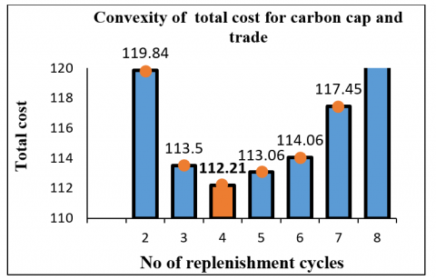
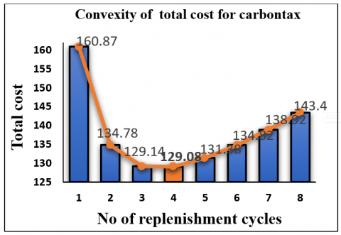
Optimal cycles for replenishment, as determined through analysis, is at n1=4. Once the minimum threshold has been reached at n1=4. Subsequently, it gradually ascends in subsequent cycles. Similarly, for the centralized (cap and trade) case, total cost of system is 112.21$ which reach its optimal level at n1=4. Tables 2 and 3 exhibit a convex pattern of the system’s cost function. This observation is further supported by graphical representations.
$\begin{gathered}T c_{\text {System }}\left(n_1, t_i\right)=n_1 *\left(O_r+S_r\right)+H_r \sum_{i=1}^{n_1} \int_{t_i}^{t_{i+1}} \int_t^{t_{i+1}}(a+ \\ b u) e^{\theta(u-t)} \mathrm{du} d t+P_r \sum_{i=1}^{n_1} \int_{t_i}^{t_{i+1}}(a+b t) e^{\theta\left(t-t_i\right)} \mathrm{dt}+ \\ \sum_{i=0}^{n_1-1} \delta\left(\hat{c}+\hat{P}_r * \int_{t_i}^{t_{i+1}}(a+b t) e^{\theta\left(t-t_i\right)} \mathrm{dt}+\widehat{h_r} \int_{t_i}^{t_{i+1}} \int_t^{t_{i+1}}(a+\right. \\ \left.b u) e^{\theta(u-t)} d u d t-CO_{2_{C a p}}\right)\end{gathered}$
$\begin{gathered}T c_{\text {System }}\left(n_1, t_i\right)=n_1 *\left(O_r+S_r\right)+\delta * \hat{c}+ \\ \left(\frac{H_r+\delta * \hat{h}_r}{\theta}+\left(P_r+\widehat{P}_r * \delta+c_p\right)\right) \sum_{i=1}^{n_1} \int_{t_i}^{t_{i+1}}(a+ \\ \text { bt) } e^{\theta\left(t-t_i\right)} \mathrm{dt}-\frac{H_r+\delta * \hat{h}_r}{\theta}\left(a * H+\frac{1}{2} * b^* H^2\right)-\delta * \\ \operatorname{CO}_{2_{\text {cap }}}\end{gathered}$ (11)
Preposition 1:
$\left(a+b t_{i+1}\right) e^{\theta\left(\mathrm{T}_{i+1}\right)}<b\left(e^{\theta\left(\mathrm{T}_i\right)}-1\right) / \theta+(a+b t) e^{\theta\left(\mathrm{T}_i\right)}$
Proof: $F\left(t_i\right)-F\left(t_{i+1}\right)<\frac{F^{\prime}\left(t_i\right)}{F\left(t_i\right)} \int_{t_i}^{t_{i+1}} F(t) d t$
Let $\mathrm{F}(\mathrm{t})=(a+b t) e^{\theta\left(\mathrm{t}-\mathrm{t}_i\right)}$ is a log convex function [21]. By putting the value of F(t) in the above equation. we have
$\begin{aligned} & \left(a+b t_{i+1}\right) e^{\theta\left(t_{i+1}-t_i\right)}-\left(a+b t_i\right)<\left(\frac{b}{\left(a+b t_i\right)}+\right. \\ & \theta) \int_{t_i}^{t_{i+1}}(a+b t) e^{\theta\left(t-t_i\right)} d t \\ & \frac{\partial T c_{\text {system }}\left(n_1, t_i\right)}{\partial t_i}=\left(a+b t_i\right)\left(e^{\theta\left(t_i-t_{i-1}\right)}-1\right) \\ & -\theta \int_{t_i}^{t_{i+1}}(a+b t) e^{\theta\left(t-t_i\right)} d t=0 \\ & \end{aligned}$
By Eq. (10) we have
$\begin{gathered}\frac{\left(a+b t_i\right)\left(e^{\theta\left(\mathrm{t}_i-t_{i-1}\right)}-1\right)}{\theta}=\int_{t_i}^{t_{i+1}}(a+b t) e^{\theta\left(\mathrm{t}-\mathrm{t}_i\right)} \mathrm{d} t \\ \left(a+b t_{i+1}\right) e^{\theta\left(T_{i+1}\right)}-\left(a+b t_i\right)<\left(\frac{b}{\left(a+b t_i\right)}+\theta\right) \\ \frac{\left(a+b t_i\right) e^{\theta\left(T_i\right)}-\left(a+b t_i\right)}{\theta} \\ \left(a+b t_{i+1}\right) e^{\theta\left(\mathrm{T}_{i+1}\right)}<\frac{b\left(e^{\theta\left(\mathrm{T}_i\right)}-1\right)}{\theta}+\left(a+b t_i\right) e^{\theta\left(\mathrm{T}_i\right)}\end{gathered}$
Lemma1:
$t_i$ strictly monotonic increase function of the last replenishment cycle $t_n$ where i=1,2,3…………. n1-1.
Proof: See Appendix A.
This lemma highlights the connection between the replenishment time, last replenishment time, length of replenishment time, and the time horizon.
$T_{i+1}=t_{i+1}-t_i$ and $t_n=\mathrm{H}-T_n$
Theorem 1: The optimal replenishment period for a fixed replenishment cycle is the unique solution that exists for the nonlinear system represented by Eq. (8).
The Hessian matrix obtained by the partial differentiation of $T c_{\text {System }}\left(n_1, t_i\right)$ it is necessary for it to be positive definite for ti to be minimum for a fixed n.
As a result, see Appendix B, the theorem establishes that $T c_{\text {System }}\left(n_1, t_i\right)$ is positive definite. Therefore, the optimum value of ti obtained using numerical iterative technique for a given fixed positive integer with mathematical programs constructed by Mathematica software version-12.0. Based on the optimal value of ti, Total cost function also will minimize.
Theorem 2: For a finite horizon planning H, the number of replenishment cycles exhibits convex behaviour of the function $T c_{\text {System }}\left(n_1, t_i\right)$.
Proof: See Appendix C.
We have already introduced an approach for determining the optimal replenishment time solution. To find the replenishment time $t_i$ put $\frac{\partial T c_{\text {System }}\left(n_1, t_i\right)}{\partial t_i}=0$. Therefore, we find the following differential equations by taking partial differentiation of $T c_{\text {System }}$ w.t.r to $t_i$, respectively.
$\begin{gathered}\frac{\partial}{\partial t_i} \mathrm{Tc}_{\text {system }}\left(n_1, t_i\right)=\left(\frac{H_r+\tau * \hat{\hbar}_r}{\theta}+\left(P_r+\hat{P}_r * \tau\right)\{(a+\right. \\ \left.\mathrm{bt}_i\right)\left(e^{\theta\left(t_i-t_{i-1}\right)}\right)-\left(a+\mathrm{bt}_{i+1}\right) e^{\theta\left(t_{t+1}-t_i\right)}+\frac{b}{\theta} e^{\theta\left(t_{i+1}-t_i\right)}- \left.\frac{b}{\theta}\right\}=0\end{gathered}$ (12)
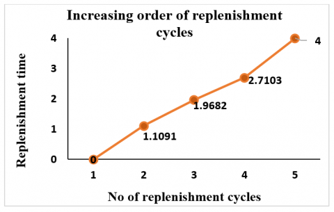
Furthermore, using the algorithms mentioned in previously published works, the optimum values of supply chain cost as a whole, n number of replenishment cycles, and total quantity of carbon emission for both policies related to emission are displayed in Tables 2 and 3, and Figures 1-3 respectively.
Using the following data, a dual-level inventory logistics network with carbon regulations within a finite planning horizon (FPH) is explored. Most of the data are identical to those used in previously published publications [6, 22].
Here is a list of fundamental parameter values along with their corresponding units. $O_r=$ $80 \$ /$ order, $H_r=0.04 \$ /$ unit/time, $P_r=0.02, \Theta=0.2, \mathrm{a}=0.5$, $\mathrm{b}=2, \widehat{h_r}=8, \quad S s=25, \mathrm{c}^{\wedge}=4, \hat{P}_r=0.7, C_p=4, \tau=$ $0.022, \delta=0.0108, \mathrm{{Co}_2}_{Cap}$$=200$. After finding the values of $t_{\text {, }}$, then to find the cost, computed the solution to the nonlinear function by numerical iterative approximation technique in "Wolfram Mathematica" a software for solving mathematical problems. Tables 2 and 3, and Figures 1-3, give a piece of comprehensive information about the optimal overall cost for an entire system. In the Decentralized (carbine tax) case, the total cost of the system is 129.08$ that reach its.
The comparative analysis of decentralized and centralized carbon policies reveals insightful findings regarding their implications for the inventory supply process. Firstly, the total cost implications indicate that the decentralized carbon tax policy tends to incur higher overall supply chain costs compared to the centralized cap-and-trade policy across all replenishment cycles. For instance, at the optimal replenishment cycle of n1=4, the total cost under the carbon tax policy amounts to \$129.08, whereas under cap-and-trade, it reduces significantly to \$112.21. Interestingly, despite differences in total cost, both policies exhibit consistent optimal replenishment cycles, indicating that the choice of policy does not substantially affect the frequency of replenishment cycles. Moreover, both carbon tax and cap-and-trade policies demonstrate similar levels of effectiveness in reducing carbon emissions within the supply chain, with minimal variation observed between the two. Sensitivity evaluations further emphasize the role of parameter adjustments in achieving reductions in overall projected emissions and costs under both carbon regimes. Notably, while there is variation in total cost between the two policies, fundamental operational aspects such as order quantity and total emissions remain relatively stable, suggesting a consistency in performance regardless of the chosen carbon policy. Overall, these comparative findings underscore the efficacy of both decentralized and centralized carbon policies in promoting sustainability and reducing carbon emissions within the inventory supply process.
Table 2. The total cost generated by the overall operator system with the emission tax, and trading policya
|
a |
n1 |
1 |
2 |
3 |
4 |
5 |
6 |
7 |
8 |
|
carbon tax |
160.87 |
134.78 |
129.14 |
129.08 |
131.38 |
134.82 |
138.92 |
143.40 |
|
|
cap and trade |
144.75 |
119.84 |
113.50 |
112.21 |
113.06 |
114.96 |
117.45 |
120.28 |
|
Table 3. The most economical and optimal number of replenishment cycles, system cost, and replenishment quantity has been computed using the policies related to carbon pricing, including carbon tax and cap-and-trade mechanisms
|
hr |
ti |
t0 |
t1 |
t2 |
t3 |
t4 |
$\boldsymbol{Amt} _{\boldsymbol {carbon }}$ |
n1 |
Qnt |
$\boldsymbol{T} \boldsymbol{c}_{\boldsymbol {System }}$ |
|
Carbon tax |
0 |
1.1091 |
1.9682 |
2.7103 |
4 |
47.6832 |
4 |
14.320 |
129.08 |
|
|
Cap and trade |
0 |
1.1091 |
1.9682 |
2.7103 |
4 |
47.6832 |
4 |
14.320 |
112.21 |
|
Figure 1. The optimal total cost generated by the overall operator system about the policy of cap and trade
Figure 2. The optimal total cost generated by the overall operator system with the carbon tax
Figure 3. The optimal replenishment time generated by the overall operator system are in increased order
6.1 Parametric analysis in the case of cap-and-trade mechanisms
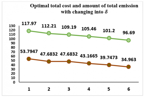
We focused to conduct sensitivity studies for several factors under the cap-and-trade framework in the discussion below. Our discussion has been confined to two factors that are directly connected, namely the carbon cap (C) and the rate of trade credit $\delta$. These variables have major impacts on the number of replenishment cycles, replenishment time, carbon emissions, and total cost.
Total cost, total amount of carbon, no replenishment cycles, and total quantity with changing $\delta$
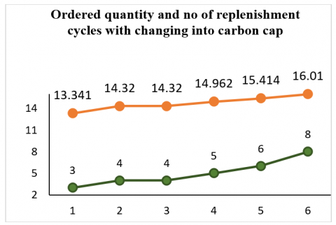
Figures 4 and 5, and Table 4 demonstrate the relationship between the $\delta$ the order quantity, number of replenishment cycles, overall system cost, and amount of carbon emission. According to the results shown, increasing $\delta$ leads to a substantial increase in the order quantity and the count of replenishment cycles, resulting in a decrease in the overall the cost of the system and the level of carbon emissions.
Total cost, total amount of carbon, no replenishment cycles, and total quantity with changing ${{CO}_2}_{Cap}$
Table 5 demonstrates that increasing the carbon cap increases the order quantity, and the number of replenishment cycles, and decreases the overall system expenses and the quantity of carbon discharge. (As seen in Figures 6 and 7) because of adjustment on provided cap. It means that decision making agencies cannot directly reduce emissions by establishing more rigorous carbon restrictions, but it may dissuade enterprises from emitting more carbon by causing considerable cost increases.
A strict cap raises the economic burden on the organization, but if the emission cap is freely allocated, the organization can minimize the overall cost by selling an unutilized quota of carbon. Figures 6 and 7 show the shifting trends of order quantity, replenishment number, the aggregate system expenditure and emission quantity.
Total cost, total amount of carbon, no replenishment cycles, and total quantity with changing $\boldsymbol\tau$
Table 6 presents the results of sensitivity analysis conducted by varying the tax paid on each unit of carbon emitted (τ). As the tax rate increases from 0.020 to 0.024, we observe changes in the optimal replenishment time (ti), the number of replenishment cycles (n1), the replenishment quantity (Qnt), and the total system cost (Tc_System).
With a tax rate of 0.020, the optimal replenishment time is distributed over eight periods, resulting in a total system cost of $150.47. As the tax rate increases to 0.021 and 0.022, the optimal replenishment time decreases, leading to a reduction in the number of replenishment cycles and the total system cost. However, beyond a tax rate of 0.022, further increases in the tax rate lead to a significant decrease in the optimal replenishment time and the total system cost.
The sensitivity analysis reveals that higher carbon taxes drive firms to optimize replenishment strategies, reducing emissions and minimizing tax burdens while maintaining efficiency. Aligning supply chain decisions with carbon regulations is crucial for cost savings and environmental sustainability.
Figure 4. The effect of change in $\delta$ on overall optimal total cost and amount of total emission of the system
Figure 5. The effect of change in $\delta$ on overall optimal ordered quantity and total number of restocking operations conducted of the system
Table 4. The most economical and optimal system cost, number of replenishment cycles, amount of emission and replenishment quantity have been calculated with changing $\delta$
|
δ |
ti |
t0 |
t1 |
t2 |
t3 |
t4 |
t5 |
t6 |
t7 |
t8 |
$\boldsymbol{Amt} _{\boldsymbol {carbon }}$ |
n1 |
Qnt |
$\boldsymbol{T} \boldsymbol{c}_{\boldsymbol {System }}$ |
|
0.0102 |
0 |
1.3151 |
2.3310 |
4 |
|
|
|
|
|
53.7947 |
3 |
13.341 |
117.97 |
|
|
0.0104 |
0 |
1.1091 |
1.9682 |
2.7103 |
4 |
|
|
|
|
47.6832 |
4 |
14.320 |
112.21 |
|
|
0.0105 |
0 |
1.1091 |
1.9682 |
2.7103 |
4 |
|
|
|
|
̶ |
4 |
̶ |
109.19 |
|
|
0.0106 |
0 |
0.9655 |
1.7155 |
2.3641 |
2.9499 |
4 |
|
|
|
43.1665 |
5 |
14.962 |
105.46 |
|
|
0.0107 |
0 |
0.8587 |
1.5279 |
2.1071 |
2.6305 |
3.1146 |
4 |
|
|
39.7473 |
6 |
15.414 |
101.20 |
|
|
0.0108 |
0 |
0.7092 |
1.2654 |
1.7478 |
2.1841 |
2.5879 |
2.9670 |
3.3266 |
4 |
34.9630 |
8 |
16.010 |
95.69 |
|
Table 5. The most economical and optimal system cost, total number of replenishment cycles carried out, amount of emission and amount for replenishment have been calculated with changing carbon cap
|
$\boldsymbol{CO}_\boldsymbol{2_{\boldsymbol{Cap}}}$ |
ti |
t0 |
t1 |
t2 |
t3 |
t4 |
t5 |
t6 |
t7 |
t8 |
$\boldsymbol{Amt} _{\boldsymbol {carbon }}$ |
n1 |
Qnt |
$\boldsymbol{T} \boldsymbol{c}_{\boldsymbol {System }}$ |
|
160 |
0 |
1.3151 |
2.3310 |
4 |
|
|
|
|
|
53.7973 |
3 |
13.341 |
119.29 |
|
|
200 |
0 |
1.1091 |
1.9682 |
2.7103 |
4 |
|
|
|
|
47.6832 |
4 |
14.320 |
112.21 |
|
|
235 |
0 |
0.9655 |
1.7155 |
2.3641 |
2.9499 |
4 |
|
|
|
43.1684 |
5 |
14.962 |
104.61 |
|
|
245 |
0 |
0.8587 |
1.5279 |
2.1071 |
2.6305 |
3.1146 |
4 |
|
|
39.7473 |
6 |
15.414 |
101.92 |
|
|
255 |
0 |
0.7758 |
1.3823 |
1.9078 |
2.3828 |
2.8224 |
3.2350 |
4 |
|
37.0886 |
7 |
15.446 |
98.85 |
|
|
260 |
0 |
0.7092 |
1.2654 |
1.7478 |
2.1841 |
2.5879 |
2.9670 |
3.3266 |
4 |
34.9631 |
8 |
16.017 |
96.65 |
|
Table 6. The most economical and optimal system cost, total number of replenishment cycles carried out, amount of emission and amount for replenishment have been calculated with changing tax paid on each unit of carbon emitted
|
t |
ti |
t0 |
t1 |
t2 |
t3 |
t4 |
t5 |
t6 |
t7 |
t8 |
$\boldsymbol{Amt} _{\boldsymbol {carbon }}$ |
n1 |
Qnt |
$\boldsymbol{T} \boldsymbol{c}_{\boldsymbol {System }}$ |
|
0.020 |
0 |
1.6399 |
4 |
|
|
|
|
|
|
150.47 |
2 |
1.6632 |
96.65 |
|
|
0.021 |
0 |
1.3151 |
2.3310 |
3 |
|
|
|
|
|
141.58 |
3 |
13.341 |
96.65 |
|
|
0.022 |
0 |
1.1091 |
1.9682 |
2.7103 |
4 |
|
|
|
|
129.08 |
3 |
14.320 |
96.65 |
|
|
0.023 |
0 |
0.7092 |
1.2654 |
1.7478 |
2.1841 |
2.5879 |
2.9670 |
3.3266 |
4 |
72.4563 |
8 |
16.010 |
96.65 |
|
|
0.024 |
0 |
0.7092 |
1.2654 |
1.7478 |
2.1841 |
2.5879 |
2.9670 |
3.3266 |
4 |
72.4563 |
8 |
16.010 |
96.65 |
|
Figure 6. The impact of change in cap on overall best possible total cost and amount of total emission of the system
Figure 7. The effect of altering in emission cap on overall best possible ordered quantity and no of replenishment cycles of the system
The sensitivity analysis results offer valuable insights into how variations in parameters impact key aspects of the system under the cap-and-trade framework. By examining the effects of changes in variables such as the carbon cap and trade credit rate, we gain a deeper understanding of their influence on critical performance metrics such as system cost, carbon emissions, replenishment cycles, and order quantities.
These insights can help decision-makers optimize their strategies for managing carbon emissions while balancing economic considerations. For example, our analysis may reveal trade-offs between minimizing system costs and reducing environmental impact, highlighting the importance of carefully selecting parameter values to achieve desired outcomes.
In comparison to past studies, our findings may align with established trends or provide new perspectives on the dynamics of carbon policies and inventory management. By identifying similarities and differences, we can enrich our understanding of the factors driving system behavior and inform future research directions.
Overall, the sensitivity analysis results contribute valuable insights that can enhance decision-making and policy formulation in the context of carbon management and inventory optimization.
In conclusion, this study provides a comprehensive examination of the optimization of a two-stage supply management system within a finite planning horizon, with a particular focus on the implications of decentralized and centralized carbon policies. Businesses, under increasing pressure due to stringent carbon regulations, are seeking strategies to reduce carbon emissions throughout their supply chains while ensuring sustainable development. The two primary approaches explored in this study, namely decentralized carbon taxation (Carbon Tax) and centralized emissions trading (cap-and-trade), represent contrasting methods for incentivizing emission reductions.
Through meticulous analysis and modeling, we have shed light on the intricate interactions between carbon policies, supply chain costs, and environmental sustainability. Our investigation has revealed that while both carbon policies aim to curb emissions and promote sustainability, they do so through different mechanisms that lead to distinct outcomes in terms of overall supply chain costs. Specifically, our findings indicate that the decentralized carbon tax policy often results in higher overall costs compared to the centralized cap-and-trade policy. This discrepancy can be attributed to the direct imposition of carbon taxes on emissions in the decentralized approach, whereas the cap-and-trade system introduces a market-based mechanism for allocating emission allowances.
However, despite differences in cost implications, both carbon policies demonstrate consistent performance in optimizing replenishment cycles and achieving reductions in carbon emissions. Sensitivity analyses conducted as part of this research underscore the significance of parameter adjustments in influencing projected emissions and costs under both carbon regimes. Furthermore, fundamental operational metrics such as order quantity and total emissions exhibit stability across different carbon policy scenarios, highlighting the robustness of the optimized supply chain strategies.
In addition to providing insights into the comparative effectiveness of carbon policies, this study contributes to the broader discourse on sustainable supply chain management. By elucidating the complex interplay between environmental objectives, regulatory frameworks, and operational dynamics, our research offers practical guidance for businesses navigating the transition towards more sustainable supply chain practices. Moreover, the methodologies and insights presented herein can serve as valuable tools for decision-makers seeking to align environmental stewardship with operational efficiency in today's increasingly carbon-constrained world.
In summary, this research advances our understanding of how different carbon policies influence supply chain dynamics and underscores the importance of integrated approaches to achieving environmental and economic sustainability. By elucidating the trade-offs and synergies inherent in decentralized and centralized carbon policies, this study empowers businesses to make informed decisions that promote both environmental stewardship and long-term competitiveness in the global marketplace.
While this study provides valuable insights into optimizing supply chain management under carbon pricing policies, several limitations should be acknowledged. Firstly, the model's assumptions, though necessary for mathematical tractability, may oversimplify real-world complexities. Additionally, the reliance on accurate and comprehensive data poses challenges, as data availability varies across industries and regions. Moreover, the scope of analysis, focusing on specific supply chain stages, may overlook broader interactions and systemic effects. Finally, the practical challenges of implementing carbon policies in diverse organizational contexts remain unaddressed.
Moving forward, Future research can explore dynamic modeling, risk integration, and multi-objective optimization for more comprehensive insights. Empirical studies can validate theoretical findings, and policy evaluations can guide stakeholders. Additionally, extending the analysis to include two-and three-echelon supply chains, and holds promise for deeper understanding and practical relevance [23, 24].
Appendix A:
Proof of Lemma 1.
Since $t_{n_1}=\mathrm{H}-T_{n_1}$
Following the studies [21, 24], we also employed the concept of mathematical induction to establish that $T_i$ increase with the $T_{n_1}=\mathrm{n}-1, \mathrm{n}-2 \ldots \ldots . .2 .1$ Put $\mathrm{i}=n_1-1$ When we put $i=n ~ 1-1$ into Eq. (10), we obtain:
$\begin{aligned} & \frac{\partial}{\partial t_i} \mathrm{Tc}_{\text {system }}\left(n_1, t_i\right)\left.=\left[a+b\left(H-T_{n_1}\right)\right] e^{\theta\left(T_{n_1-1}\right.}\right) \\ &- {\left[a+b\left(H-T_{n_1}\right) \theta \int_{H-T_{n_1}}^H(a\right.} \\ &+b t) e^{\theta\left(t-H+T_{n_1}\right)} d t=0\end{aligned}$
Then differentiate Eq. (10) w.r.t $T_{n_1}$
$\begin{gathered}{\left[a+b\left(\mathrm{H}-T_{n_1}\right)\right] e^{\theta\left(T_{n_1-1}\right)} \frac{d\left(T_{n_1-1}\right)}{d T_{n_1}}-b e^{\theta\left(T_{n_1-1}\right)}+b-} \\ {\left[a+b\left(\mathrm{H}-T_{n_1}\right)\right]-\theta^2 \int_{\mathrm{H}-T_{n_1}}^{\mathrm{H}}(a+b t) e^{\theta\left(\mathrm{t}-\mathrm{H}+T_{n_1}\right)} \mathrm{d} t=0}\end{gathered}$ (A1)
$\left(a+b t_i\right)\left(e^{\theta\left(\mathrm{t}_i-t_{i-1}\right)}-1\right)=\theta \int_{t_i}^{t_{i+1}}(a+b t) e^{\theta\left(\mathrm{t}-\mathrm{t}_i\right)} \mathrm{d} t$
We get by Eq. (10) and then put in Eq. (A1)
$\begin{gathered}{\left[a+b\left(H-T_{n 1}\right)\right] e^{\theta\left(T_{n-1}\right)} \frac{d\left(T_{n 1}-1\right)}{\mathrm{dT}_{n_1}}} \\ =b\left(e^{\theta\left(T_{n 1}-1\right)}-1\right) \\ +\theta\left[a+\left(H-T_{n 1}\right)\right] e^{\theta\left(T_{n 1}-1\right)} \\ \theta\left[a+b\left(\mathrm{H}-T_{n_1}\right)\right] e^{\theta\left(T_{n_1-1}\right)}\left\{\frac{d\left(T_{n_1-1}\right)}{d T_{n_1}}-1\right\}=b\left(e^{\theta\left(T_{n_1-1}\right)}-1\right) \\ \left\{\frac{d\left(T_{n_1-1}\right)}{d T_{n_1}}\right\}=\frac{b\left(e^{\theta\left(T_{n_1-1}\right)}-1\right)}{\theta\left[a+b\left(\mathrm{H}-T_{n_1}\right)\right] e^{\theta\left(T_{n_1-1}\right)}+1}\end{gathered}$
$\frac{d\left(T_{n_1-1}\right)}{d T_{n_1}}=\frac{b\left(e^{\theta\left(T_{n_1-1}\right)_{-1}}-\theta\left[a+b\left(\mathrm{H}-T_{n_1}\right)\right] e^{\theta\left(T_{n_1-1}\right)}\right.}{\theta\left[a+b\left(\mathrm{H}-T_{n_1}\right)\right] e^{\theta\left(T_{n_1-1}\right)}} \geq 0$ (A2)
After that, let's us take that $\frac{\mathrm{d}\left(\mathrm{T}_{\mathrm{m}}\right)}{\mathrm{dT}_{n_1}}>0$ for $\mathrm{m}=\mathrm{i}+1, \mathrm{i}+2, \ldots \ldots$, $n_1-1$ And then again differentiate Eq. (20) w.r.t $\mathrm{T}_{n_1}$, we have
$\begin{array}{*{35}{r}} b\left( {{e}^{\theta \left( {{T}_{i}} \right)}}-1 \right)\frac{d\left( {{t}_{i}} \right)}{dT{{n}_{1}}}+\theta \left( a+b{{t}_{i}} \right){{e}^{\theta \left( {{T}_{i}} \right)}}\frac{d\left( {{T}_{i}} \right)}{d{{T}_{{{n}_{1}}}}}-\theta \left( a+b{{t}_{i+1}} \right){{e}^{\theta \left( {{T}_{i+1}} \right)}}\frac{d\left( {{t}_{i+1}} \right)}{d{{T}_{{{n}_{1}}}}}+ \\ \theta \left( a+b{{t}_{i}} \right)\frac{d\left( {{t}_{i}} \right)}{d{{T}_{{{n}_{1}}}}}+{{\theta }^{2}}\frac{d\left( {{t}_{i}} \right)}{d{{T}_{{{n}_{1}}}}}\int_{{{t}_{1}}}^{{{t}_{i+1}}}{(a+bt)}{{e}^{\theta \left( t-{{t}_{i}} \right)}}dt \\\end{array}$ (A3)
By using preposition and Eq. (10)
$\frac{d\left(t_i\right)}{d T_{n_1}} \leq \frac{d\left(t_{i+1}\right)}{d T_{n_1}}=-\sum_{m=i+2}^{n_1-1} \frac{d\left(T_m\right)}{d T_{n_1}}-1 \leq 0$ (A4)
This implies $\frac{d\left(T_i\right)}{d T_{n_1}} \geq 0$ where $\mathrm{i}=1,2,3 \ldots \ldots \ldots \ldots \ldots n_1-1$.
Moreover, as we know that $T_{n_1}=\mathrm{H}-t_{n_1-1}$ this implies $\frac{d\left(T_i\right)}{d T_{n_1-1}} \leq 0$ where $\mathrm{i}=1,2,3 \ldots \ldots \ldots \ldots . . .$.
Now, we take
$t_i=H-\sum_{m=i+1}^{n_1-1} T_u-T_{n_1}=t_{n_1-1}-\sum_{m=i+1}^{n_1-1} T_u$
from this it is concluded that $\frac{d\left(t_i\right)}{d t_{n_1}} \geq 0$, for all $\mathrm{i}=1,2,3 \ldots \ldots \ldots \ldots . . . . n_1-1$.
Appendix B:
We need verify the following to justify Theorem 1.
The intention of calculating $t_i$ values is to prove the system's total variable cost $T c_{\text {System }}\left(n_1, t_i\right)$ is a convex function. The first and most important prerequisite for obtaining $t_i$ is to establish that the
$\frac{\partial}{\partial_{t_i}} T c_{\text {System }}\left(n_1, t_i\right)=0$
$\begin{aligned} & \frac{\partial}{\partial_{t_i}} T c_{\text {System }}\left(n_1, t_i\right)=\left(\frac{H_r+\tau * \widehat{h_r}}{\theta}+\left(P_r+\hat{P}_r\right.\right. * \tau))\left\{\left(a+b t_i\right)\left(e^{\theta\left(t_i-t_{i-1}\right)}\right)\right. \\ & \left.-\left(a+b t_{i+1}\right) e^{\theta\left(t_{i+1}-t_i\right)}+\frac{b}{\theta} e^{\theta\left(t_{i+1}-t_i\right)}-\frac{b}{\theta}\right\}=0 \\ & \frac{\partial^2 T c_{\text {System }}\left(n_1, t_i\right)}{\partial t_i{ }^2}=\left(b\left(e^{\theta\left(t_i-t_{i-1}\right)}-1\right)+\theta(a+\right. \\ & \left.\left.b t_i\right) e^{\theta\left(t_i-t_{i-1}\right)}+\theta\left(a+b t_i\right)+\theta^2 \int_{t_i}^{t_{i+1}}(a+b t) e^{\theta\left(t-t_i\right)} \mathrm{dt}\right) \\ & \end{aligned}$
$\begin{gathered}\frac{\partial^2 \mathrm{Tc}_{\text {system }}\left(n_1, t_i\right)}{\partial t_i^2}=\theta\left(a+\mathrm{bt}_i\right) e^{\theta T_i}+\theta(a+ \left.t_{i+1}\right) e^{\theta T_{i+1}}+b\left(e^{\theta T_i}-e^{\theta T_{i+1}}\right)\end{gathered}$ (B1)
$\frac{\partial^2 T c_{\text {System }}\left(n_1, t_i\right)}{\partial t_i \partial t_{i+1}}=-\theta\left(a+b t_{i+1}\right) e^{\theta T_{i+1}}$ (B2)
$\frac{\partial^2 T c_{\text {System }}\left(n_1, t_i\right)}{\partial t_i \partial t_{i+1}}=-\theta\left(a+b t_{i+1}\right) e^{\theta T_{i+1}}$ (B3)
$\frac{\partial^2 T c_{\text {System }}\left(n_1, t_i\right)}{\partial t_i \partial t_m}=0$ for all $\mathrm{m} \neq \mathrm{i}, \mathrm{i}+1, \mathrm{i}-1$ (B4)
Furthermore,
$\nabla^2 T c_{\text {System }}\left(n_1, t_i\right)=\left[\begin{array}{ccccccccc}\frac{\partial^2 T c_{\text {System }}}{\partial t_1^2} & \frac{\partial^2 T c_{\text {System }}}{\partial t_1 \partial t_2} & 0 & 0 & 0 & 0 & 0 & 0 & 0 \\ \frac{\partial^2 T c_{\text {System }}}{\partial t_2 \partial t_1} & \frac{\partial^2 T c_{\text {System }}}{\partial t_2^2} & \frac{\partial^2 T c_{\text {System }}}{\partial t_2 \partial t_3} & 0 & 0 & 0 & 0 & 0 & 0 \\ 0 & \frac{\partial^2 T c_{\text {System }}}{\partial t_3 \partial t_2} & \frac{\partial^2 T c_{\text {System }}}{\partial t_3^2} & \frac{\partial^2 T c_{\text {System }}}{\partial t_3 \partial t_4} & 0 & 0 & 0 & 0 & 0 \\\cdots & \cdots & \cdots & \cdots & \cdots & \cdots & \cdots & \cdots & \cdots \\ \\0 & 0 & 0 & 0 & 0 & 0 & 0 & 0 & 0\\0 & 0 & 0 & 0 & 0 & 0 & \frac{\partial^2 T c_{\text {System }}}{\partial t_{n_{1-1}} \partial t_{n_{1-2}}} & \frac{\partial^2 T c_{\text {System }}}{\partial t_{n_{1-1}}^2} & \frac{\partial^2 T c_{\text {System }}}{\partial t_{n_{1-1}} \partial t_{n_1}} \\ 0 & 0 & 0 & 0 & 0 & 0 & 0 & \frac{\partial^2 T c_{\text {System }}}{\partial t_{n_1} \partial t_{n_{1-1}}} & \frac{\partial^2 T c_{\text {System }}}{\partial t_{n_1}^2}\end{array}\right]$
$T C_s$ is positive definite if Eq. $\left(\mathrm{B}_1\right)$, Eq. $\left(\mathrm{B}_2\right)$, Eq. $\left(\mathrm{B}_3\right)$, and Eq. $\left(\mathrm{B}_4\right)$, satisfy the given inequality.
$\begin{aligned}
& \frac{\partial^2 T c_{\text {System }}}{\partial t_i^2} \geq\left|\frac{\partial^2 T c_{\text {System }}}{\partial t_i t_{i-1}}\right|+\left|\frac{\partial^2 T c_{\text {System }}}{\partial t_i t_{i+1}}\right| \frac{\partial^2 T c_{\text {System }}}{\partial t_i^2} \\
& -\left|\frac{\partial^2 T c_{\text {System }}}{\partial t_i t_{i-1}}\right|-\left|\frac{\partial^2 T c_{\text {System }}}{\partial t_i t_{i+1}}\right| \geq 0 \\
& \theta\left(a+b t_i\right) e^{\theta T_i}+\theta\left(a+b t_{i+1}\right) e^{\theta T_{i+1}}+b\left(e^{\theta T_i}-\right. \\
& \left.e^{\theta T_{i+1}}\right)-\theta\left(a+b t_i\right) e^{\theta T_i}-\theta\left(a+b t_{i+1}\right) e^{\theta T_{i+1}}>0 \\
& b\left(e^{\theta T_i}-e^{\theta T_{i+1}}\right)>0 \\&\end{aligned}$
that is true for all i=1, 2, . . ., n
Moreover, the Hessian matrix had to be positive definite since it contains positive diagonal members and has strictly diagonal dominating features. As a result, the optimal replenishment interval to the nonlinear system of Eq. (10) is obtained. now we need to show that the optimal solution of the non-linear Eq. (10) is unique and also $T c_{\text {System }}\left(\mathrm{t}_{\mathrm{i}}, \mathrm{n}\right)$ is optimal function throughout the optimal value of ti in a finite horizon planning H.
Furthermore, because it had strictly diagonal dominating characteristics and positive diagonal members, the Hessian matrix required to be positive definite. As a result, the optimum replenishment interval for nonlinear system Eq. (10) is established. Now we need to demonstrate the convexity of $T c_{\text {System }}\left(\mathrm{t}_{\mathrm{i}}, \mathrm{n}\right)$ throughout the optimal value of ti in the finite horizon planning H.
Appendix C
To validate Theorem 2, we need establish the following:
With the procedure., we have
$\begin{gathered}T c_{\text {System }}\left(n_1, t_i\right)=n_1 *\left(O_r+S_r\right)+\tau * \hat{c}+\left(\frac{H_r+\tau * \widehat{h_r}}{\theta}+\right. \\ \left.\left(P_r+\hat{P}_r * \tau+C_p\right)\right) \sum_{i=1}^{n_1} \int_{t_i}^{t_{i+1}}(a+ \\ b t) e^{\theta\left(t-t_i\right)} \mathrm{dt}-\frac{H_r+\tau * \widehat{h_r}}{\theta}\left(a * H+\frac{1}{2} * b * H^2\right)\end{gathered}$
where, t0=0 and $\mathrm{t} n_1=\mathrm{H}$.
Let us now suppose,
$\begin{gathered}T_{\text {Ret }}\left(t_i, n\right)=n_1 *\left(O_r+S_r\right) \\+\left(\frac{H_r+\tau * \widehat{h_r}}{\theta}+\left(P_r+\widehat{P}_r * \tau\right.\right. \\\left.\left.+C_p\right)\right) \sum_{i=1}^{n_1} \int_{t_i}^{t_{i+1}}(a+b t) e^{\theta\left(t-t_i\right)} \mathrm{dt}+K \\\text { where, } \tau * \hat{c}-\frac{H_r+\tau * \widehat{h_r}}{\theta}\left(a * H+\frac{1}{2} * b * H^2\right)=K \\F\left(n_1, 0, H\right)=\sum_{i=1}^{n_1} \int_{t_i}^{t_{i+1}}(a+b t) e^{\theta\left(t-t_i\right)} \mathrm{dt} \\b t) e^{\theta\left(t-t_{n_1-1}\right)} \mathrm{dt}+\int_{t_{n_1}}^{\mathrm{T}}(a+b t) e^{\theta\left(t-t_{n_1}\right)} \mathrm{dt}-\int_{t_{n_1-1}}^{\mathrm{T}}(a+b t) e^{\theta\left(t-t_{n_1-1}\right)} \mathrm{dt} \\F\left(n_1+1,0, H\right)-F\left(n_1, 0, \mathrm{H}\right)=\int_{t_{n_1}}^T(a+\mathrm{bt})\left\{e^{\theta\left(t-t_{n_1}\right)}-e^{\theta\left(t-t_{n_1-1}\right)}\right\} \mathrm{dt}<0 \\F\left(n_1+1,0, H\right)-F\left(n_1, 0, H\right)<0 \\F\left(n_1+1,0, H\right)<F\left(n_1, 0, H\right)\end{gathered}$
Let us considered
$\begin{gathered}F\left(n_1, 0, H\right)-F\left(n_1-1,0, H\right)-\left[F\left(n_1+1,0, H\right)-F\left(n_1, 0, H\right)\right]= \\ \int_{t_{n_1-1}}^T(a+b t)\left[e^{\theta\left(t-t_{n_1-1}\right)}-e^{\theta\left(t-t_{n_1-2}\right)}\right] \mathrm{dt}-\int_{t_{n_1}}^T(a+ \\ b t)\left[e^{\theta\left(t-t_{n_1}\right)}-e^{\theta\left(t-t_{n_1-1}\right)}\right] \mathrm{dt}=\int_{t_{n_1-1}}^T(a+b t)\left[e^{\theta\left(t-t_{n_1-1}\right)}-\right. \\ \left.e^{\theta\left(t-t_{n_1-2}\right)}\right] \mathrm{dt}+\int_{t_{n_1}}^T(a+b t)\left[e^{\theta\left(t-t_{n_1-1}\right)}-e^{\theta\left(t-t_{n_1-2}\right)}\right] \mathrm{dt}- \\ \int_{t_{n_1}}^T(a+b t)\left[e^{\theta\left(t-t_{n_1}\right)}-e^{\theta\left(t-t_{n_1-1}\right)}\right] \mathrm{dt}\end{gathered}$
$\begin{gathered}F\left(n_1, 0, H\right)-F\left(n_1-1,0, H\right)-\left[F\left(n_1+1,0, H\right)-F\left(n_1, 0, H\right)\right] \\ \left.=\int_{t_{n_1-1}}^T(a+b t)\left[e^{\theta\left(t-t_{n_1-1}\right)}-e^{\theta\left(t-t_{n_1-2}\right.}\right)\right] \mathrm{dt} \\ +\int_{t_{n_1}}^T(a+b t)\left[2 e^{\theta\left(t-t_{n_1-1}\right)}-e^{\theta\left(t-t_{n_1}\right)}\right. \\ \left.-e^{\theta\left(t-t_{n_1-2}\right)}\right] \mathrm{dt}<0 \\ F\left(n_1, 0, H\right)-F\left(n_1-1,0, H\right)-\left[F\left(n_1+1,0, H\right)-F\left(n_1, 0, H\right)\right]<0 \\ F\left(n_1, 0, H\right)-F\left(n_1-1,0, H\right)<F\left(n_1+1,0, H\right)-F\left(n_1, 0, H\right)\end{gathered}$
Since $e^t$ is a convex function, $\mathrm{F}\left(n_1, 0, \mathrm{H}\right)$ is a convex function in $n_1$. This indicates that $T c_{\text {System }}\left(t_i, n\right)$ is Inherently a convex function.
[1] Kumar, B.K., Nagaraju, D., Narayanan, S. (2016). Three-echelon supply chain with centralised and decentralised inventory decisions under linear price dependent demand. International Journal of Logistics Systems and Management, 23(2): 231-254., https://doi.org/10.1504/IJLSM.2016.073970
[2] Nagaraju, D., Rao, A.R., Narayanan, S. (2016). Centralised and decentralised three echelon inventory model for optimal inventory decisions under price dependent demand. International Journal of Logistics Systems and Management, 23(2): 147-170. https://doi.org/10.1504/IJLSM.2016.073966
[3] Oluwaseyi, J.A., Onifade, M.K., Odeyinka, O.F. (2017). Evaluation of the role of inventory management in logistics chain of an organisation. LOGI-Scientific Journal on Transport and Logistics, 8(2): 1-11., https://doi.org/10.1515/logi-2017-0011
[4] Ghosh, A., Jha, J.K., Sarmah, S.P. (2020). Production-inventory models considering different carbon policies: A review. International Journal of Productivity and Quality Management, 30(1): 1-27. https://doi.org/10.1504/IJPQM.2020.107280
[5] Wang, X., Zhu, Y., Sun, H., Jia, F. (2018). Production decisions of new and remanufactured products: Implications for low carbon emission economy. Journal of Cleaner Production, 171: 1225-1243. https://doi.org/10.1016/j.jclepro.2017.10.053
[6] Shi, Y., Zhang, Z., Chen, S.C., Cárdenas-Barrón, L.E., Skouri, K. (2020). Optimal replenishment decisions for perishable products under cash, advance, and credit payments considering carbon tax regulations. International Journal of Production Economics, 223: 107514. https://doi.org/10.1016/j.ijpe.2019.09.035
[7] Benjaafar, S., Li, Y., Daskin, M. (2012). Carbon footprint and the management of supply chains: Insights from simple models. IEEE Transactions on Automation Science and Engineering, 10(1): 99-116. https://doi.org/10.1109/TASE.2012.220330
[8] Kung, F.C., Ju, C.Y., Dye, C.Y. (2018). Carbon-constrained deteriorating inventory model when inventory stimulates demand. International Journal of Information and Management Sciences, 29(1): 57-88. https://doi.org/10.6186/IJIMS.2018.29.1.3
[9] Mishra, N.K. (2022). A supply chain inventory model for deteriorating products with carbon emission-dependent demand, advanced payment, carbon tax and cap policy. Mathematical Modelling of Engineering Problems, 9(3). https://doi.org/10.18280/mmep.090308
[10] Kushwaha, S., Ghosh, A., Rao, A.K. (2020). Collection activity channels selection in a reverse supply chain under a carbon cap-and-trade regulation. Journal of Cleaner Production, 260: 121034. https://doi.org/10.1016/j.jclepro.2020.121034
[11] Cheng, Y., Mu, D., Zhang, Y. (2017). Mixed carbon policies based on cooperation of carbon emission reduction in supply chain. Discrete Dynamics in Nature and Society, 2017. https://doi.org/10.1155/2017/4379124
[12] Sarkar, B., Saren, S., Sinha, D., Hur, S. (2015). Effect of unequal lot sizes, variable setup cost, and carbon emission cost in a supply chain model. Mathematical Problems in Engineering, 2015. https://doi.org/10.1155/2015/469486
[13] Yan, B., Wang, T., Liu, Y.P., Liu, Y. (2016). Decision analysis of retailer-dominated dual-channel supply chain considering cost misreporting. International Journal of Production Economics, 178: 34-41. https://doi.org/10.1016/j.ijpe.2016.04.020
[14] Bai, Q., Xu, J., Meng, F., Yu, N. (2021). Impact of cap-and-trade regulation on coordinating perishable products supply chain with cost learning. Journal of Industrial & Management Optimization, 17(6). https://doi.org/10.3934/jimo.2020126
[15] Hovelaque, V., Bironneau, L. (2015). The carbon-constrained EOQ model with carbon emission dependent demand. International Journal of Production Economics, 164: 285-291. https://doi.org/10.1016/j.ijpe.2014.11.022
[16] Hua, G., Cheng, T.C.E., Wang, S. (2011). Managing carbon footprints in inventory management. International Journal of Production Economics, 132(2): 178-185. https://doi.org/10.1016/j.ijpe.2011.03.024
[17] Xu, L., Wang, C., Zhao, J. (2018). Decision and coordination in the dual-channel supply chain considering cap-and-trade regulation. Journal of Cleaner Production, 197: 551-561. https://doi.org/10.1016/j.jclepro.2018.06.209
[18] Qin, J., Bai, X., Xia, L. (2015). Sustainable trade credit and replenishment policies under the cap-and-trade and carbon tax regulations. Sustainability, 7(12): 16340-16361. https://doi.org/10.3390/su71215818
[19] Ghosh, A., Jha, J.K., Sarmah, S.P. (2017). Optimal lot-sizing under strict carbon cap policy considering stochastic demand. Applied Mathematical Modelling, 44: 688-704. https://doi.org/10.1016/j.apm.2017.02.037
[20] Toptal, A., Çetinkaya, B. (2017). How supply chain coordination affects the environment: A carbon footprint perspective. Annals of Operations Research, 250: 487-519. https://doi.org/10.1007/s10479-015-1858-9
[21] Hariga, M. (1996). Optimal EOQ models for deteriorating items with time-varying demand. Journal of the Operational Research Society, 47(10): 1228-1246. https://doi.org/10.1057/jors.1996.151
[22] Wu, C., Zhao, Q. (2014). Supplier–retailer inventory coordination with credit term for inventory‐dependent and linear‐trend demand. International Transactions in Operational Research, 21(5): 797-818. https://doi.org/10.1111/itor.12060
[23] Mishra, N.K., Jain, P. (2024). Blockchain-Enhanced inventory management in decentralized supply chains for finite planning horizons. Journal Européen des Systèmes Automatisés, 57(1): 263-272. https://doi.org/10.18280/jesa.570125
[24] Mishra, N.K., Ranu. (2023). A supply chain inventory model for a deteriorating material under a finite planning horizon with the carbon tax and shortage in all cycles. Journal Européen des Systèmes Automatisés, 56(2): 221-230. https://doi.org/10.18280/jesa.560206