Ahmed Hamet Sidi![]() | Mohammed Abd El Djalil Djehaf*
| Mohammed Abd El Djalil Djehaf*![]() | Youcef Islam Djilani Kobibi
| Youcef Islam Djilani Kobibi![]()
© 2024 The authors. This article is published by IIETA and is licensed under the CC BY 4.0 license (http://creativecommons.org/licenses/by/4.0/).
OPEN ACCESS
Accurate tracking of ball trajectories on a platform using a 2-DOF balancer system poses significant challenges in the existing literature due to its inherent nonlinearity and instability. This research addresses these challenges through a two-fold approach. Firstly, we focus on designing a robust 2-DOF ball balancer system model. Secondly, we perform a comparative study of three control techniques: Linear Quadratic Regulator-based Proportional (LQR_P), Full State Feedback-based Proportional (FSF_P), and Classical Proportional Derivative-based Proportional (PD_P) control. To evaluate the effectiveness of the designed controllers, we conduct both simulation and experimental tests using MATLAB Simulink integrated with Quarc software and the 2DOF ball balancer system Quanser hardware. The results demonstrate that the Linear Quadratic Regulator-based proportional control exhibits superior performance in terms of transient response, including percentage overshoot, settling time, and peak time. Moreover, it showcases excellent steady-state response, achieving a minimum steady-state error of 0.641mm, outperforming the other techniques investigated in this study.
trajectory tracking, ball balancer, proportional derivative control, linear quadratic regulator, full state feedback control
The 2-DOF ball balancer system is a didactic platform commonly employed in research laboratories and academic settings to assess the performance and effectiveness of control techniques. Utilizing visual system-based imaging, it finds applications in diverse fields, including robotics, such as assembly robots, military applications, surgical procedures, and aerospace industries. The system is characterized as underactuated, electromechanical, decoupled, highly nonlinear, and inherently unstable, presenting substantial challenges for trajectory control and stabilization.
The ball balancer consists of a free-moving ball atop a plate-beam system, lacking the ability to perceive its environment [1]. These factors collectively contribute to the inherent challenge of accurately controlling the ball's position. Moreover, constructing a precise mathematical model that describes the system has been a formidable task. Numerous researchers have explored the design of the ball and plate system and have experimented with various approaches to control the system within specific time domains, including settling time, peak time, percentage overshoot, and minimum steady-state error.
Such as study [1], trajectory tracking of ball-based switching control technique and nonlinear analysis was carried. Ker et al. [2] generated the control law and back-stepping controller to achieve the performance of the system. Steady state error response was compared with two approaches, standard PID controller and generalized Kalman-Yanukovych-Popov lemma approach [3]. Later on, point to point control of the system based on a non-linear PID controller has been studied [4]. Wang et al. [5] used a double loop structured respectively fuzzy logic controller in the outer loop and a switching technique in the inner one. The issue of the fuzzy logic system its required knowledge about the system and a good choice of membership function. Shiratori et al. [6] presented a quantized feedback control system with a discrete variable quantizer with the help of model predictive control (MPC). Subramanian et al. [7] uniform bounded ultimate controller-based model reference adaptive PID to avoid plant disturbances and modeling error. Sliding mode controller was compared with a conventional proportional integral controller of one degree of freedom ball balancer system [8]. An observer integrated Backstepping controller in the form of a cascade was developed by Ma et al. [9]. Linear extended state observer and tracking differentiator were used to estimate the uncertainties of the model and derivative of the virtual control law. Singh and Bhushan [10] investigated performance comparison in the time domain between Neural integrated fuzzy logic, its hybridization with PID and a conventional PID controller. Experiment results show that neural integrated fuzzy logic has less overshoot compared to other controllers. However, all the designed controllers presented an oscillation response with a steady state error greater than 1 cm.
The issue of ball trajectory tracking remains a challenge in literature due to the complexity, saturation of the actuator and flexibility of the system to disturbance but also results in the design model. Discrete Laguerre based linear MPC optimization by moving time window control to reduce the settling time [11]. Singh and Bhushan [12] presented an improved ant colony optimization (ACO) by revising its transition probability to improve the response and convergence speed of the algorithm resulting to optimize the proportional integral derivative controller (PID) controller. And the study [13] presented a simultaneous perturbation stochastic approximation (SPSA) approach for unknown but bounded disturbances in a typical closed loop system. The proposed SPSA method minimizes the optimization problem achieving adaptive control, by computing the optimal gain values to the PID controller and stability analysis is carried out considering the linear matrix inequalities and Lyapunov stability. Fast state space model predictive control compared with LQR and conventional PID controller performance based on 2DOF ball balancer system in the study [14]. MPC manipulated variables are found online using explicit formulas with parameters calculated offline. Ali et al. [15] used a nonlinear model reference controller on 2DOF ball balancer to track the position and stability was performed based on Lyapunov. Dong et al. [16] combined fuzzy logic, neural networks, and genetic algorithms (GA) to stabilize the ball on top of the plate at a desired position. Five layers, error and change in error were used as input and the backpropagation training is used in the neural network. Conventional PID gain was also tun by fuzzy logic [17], and artificial neural networks [18].
These methods, however, prioritize preserving the more advantageous generations, leading to local rather than global optimum conditions. Additionally, there are issues brought on by intelligent controllers' weight adjustments, a lack of memory, early convergence, and poor local search.
In the study [19], nonlinear control technique backstepping and switching techniques respectively to the outer and inner loop of the ball and plate platform BPVS-JLU-II system. Fuzzy logic was added in the inner loop to decrease the steady state error, with PD controllers and bang-bang control is used to quicken up the system response. The study [20] presented a linear control law based on a reduced-order observer for friction compensation of the ball and plate system. The study [21] used genetic algorithms to design a fault-tolerant controller that has the ability to adapt to the fault condition. The three dimensions lookup table related to the current ball position, ball velocity, and plate angle to the plate angular velocity were used to control the ball motion. Fan and Han [22] presented nonlinear model predictive control based on gaussian particle swarm optimization. The gaussian particle swarm optimization was used dynamically to perform the nonlinear constraint optimization. Okafor et al. [23] proposed an artificial intelligence-based deep reinforcement learning (RL) to tun the proportional, integral, derivative gain of PID controller were compared with genetic algorithm-based PID (GA-PID) and classical PID.
As seen in the trajectory tracking with a small steady state error remained a challenge with the ball and plate system.
Pattanapong and Deelertpaiboon [24] used fuzzy logic with adaptive integral action. Sliding mode controller that includes error integration, which makes the system robust against external disturbances design to achieve the performance of the ball balancer system [25]. Hierarchical fuzzy CMAC neural networks are used to propose an indirect adaptive control method [26]. Recently, the studies [27, 28] in comparison to simple sliding mode controller and linearized sliding mode controller, which determine the beam angle from ball position, fractional order sliding mode controllers offer higher tracking precision, shorter response times, less chattering, and excellent efficiency. Pasha and Mija [29] used a linear quadratic regulator for asymptotic stability on 4 DOF ball balancer system. Kalman filter and linear quadratic regulator were used to achieve the performance of the ball balancing system [30].
Because of its intrinsic complexity, the ball balancer system includes problems such as balancing the ball on a plate and point stabilization control, which take the ball to a precise place and retain it there while minimizing tracking error and time response.
This paper investigated on performance comparison of the designed controllers on ball balancer system. This Work concentrated firstly on modelling of ball balancer setup in time domain and secondly plan on designing and implementation of controllers for system setup using Simulink integrated Quarc and in real-time as well.
The Adaptation of these controllers to ball balancer Model tend to be a Nobel.
Further sections of the paper are organized as follows:
Section 2 discusses the modeling of the ball plate system and its working principle. Section 3 designs Linear Quadratic Regulator-based Proportional (LQR_P), Proportional Derivative-based Proportional (PD_P) and Full State Feedback-based Proportional (FSF_P) for analyzing the slope of the ball position, slope of angular position and Energy consumption one. Section 4 comes up with simulation results and the stability analysis and discusses simulation and the real-time implementation of 2-DOF ball balancer. The conclusion, future works and references in Section 5.
A common benchmark problem for balancing control, ball position monitoring, and visual servo control is a ball on a plate system. The representation of the ball and plate system is typically given in Figure 1.
Figure 1. Ball-Plate system representation
The ball and plate are a nonlinear, electromechanical, multivariable, open-loop unstable system that is being studied in order to control the position of the ball by tuning the plate angle which is related to serv02 motor angle. A digital USB camera is used to capture the two-dimension x and y axis and a vision algorithm computes the reads the ball coordinates from the image and provides information to the controller.
2.1 Mathematical modeling of plant model
Time continuous state space model is developed to model the ball plate system but under certain assumptions were considered:
1. The output of the servo motor is the input of the beam plate system.
2. No Slipping Assumption: This implies that the ball maintains a rolling motion without sliding over the plate surface. It suggests a perfect transfer of rotational motion from the ball to linear motion across the plate, which is critical for maintaining control predictability and system stability in our model.
3. No Friction Assumption: We consider the interface between the ball and the plate as ideally smooth, effectively ignoring the frictional forces that might oppose the ball's motion. This simplification allows us to focus on the primary dynamics of the system without the complexities introduced by frictional calculations.
These assumptions play a pivotal role in decoupling the system's axes, simplifying the mathematical model by reducing the number of parameters needed to describe the behavior of the ball balancer system effectively. Our analysis focuses primarily on one axis (x-axis) because the x and y axes are inherently decoupled in this system, and studying one axis provides sufficient insight into the system's dynamics.
These assumptions underline on decoupling the system axis but also reduce the parameters in the model of ball balancer system. The observation and analysis were made on one axis x, since x and y axis are in nature decouple and one axis is sufficient to represent the behavior of the ball balancer system. Figure 2 shows the typical system.
Figure 2. Ball balancer free body diagram
2.2 Equation of motion using first principal
The equation of motion of the ball is determined using Newton’s second law:
$\mathrm{m}_{\mathrm{b}} \ddot{\mathrm{a}}=\sum F_{\text {ext }}=\mathrm{P}_{\mathrm{x}}-\mathrm{F}_{\mathrm{x}}$ (1)
$m_b$ denoted the mass of the ball, $\ddot{a}$ its acceleration, $P_x$ is the force due to the gravity and $F_x$ inertia force of the ball. Figure 3 shows the free body diagram of ball relates to its forces and the plate inclined with a certain angle $\alpha$.
Figure 3. Typical free body of ball plate
The force due to the gravity along the x-axis is:
$P_x=m_b G \sin (\alpha(t))$ (2)
The inertia force due to the torque is given as:
$\mathrm{F}_{\mathrm{x}}=\frac{\mathrm{J}_{\mathrm{b}}}{\mathrm{R}_{\mathrm{b}}} \frac{\mathrm{d}^2}{\mathrm{dt}^2} \gamma_{\mathrm{b}}(\mathrm{t})$ (3)
The expression of the torque from Eq. (3)
$\gamma_b(t)=\frac{1}{R_b} x(t)$ (4)
The motion equation of the ball on the top of the plate is formulated as:
$\ddot{\mathrm{X}}(\mathrm{t})=\frac{\mathrm{m}_{\mathrm{b}} \mathrm{G}}{\left(\frac{\mathrm{J}_{\mathrm{b}}}{\mathrm{R}_{\mathrm{b}}{ }^2}+\mathrm{m}_{\mathrm{b}}\right)} \sin \alpha(\mathrm{t})$ (5)
2.3 Determination of the servo angle
Let’s develop the equation of motion that relates the serv02 motor angle (servo load angle) to the plate angle (beam angle). Since it’s a nonlinear system with trigonometric sinus terms. Then consider the serv02 angle needed to change the height $\mathrm{H}_{\mathrm{arm}}$ of the beam to move the ball at a certain distance x on the plate.
From the free body beam plate system:
$\mathrm{H}_{\mathrm{arm}}=\frac{\mathrm{L}_{\text {table }}}{2} \sin (\alpha(\mathrm{t}))$ (6)
The expression of the serv02 angle with respect to height:
$\mathrm{H}_{\mathrm{arm}}=\mathrm{r}_{\mathrm{arm}} \sin \theta_l(\mathrm{t})$ (7)
Equating expressions (6) and (7) by taking away $\sin \alpha(t)$
$\sin \alpha(\mathrm{t})=\frac{2 \mathrm{r}_{\mathrm{arm}}}{\mathrm{L}_{\mathrm{table}}} \sin \theta_{\mathrm{l}}(\mathrm{t})$ (8)
where, $r_{\text {arm }}$ is the distance between the coupled joint and the shaft of the SRV02 output gear, and $\mathrm{L}_{\text {table }}$ is the length of the plate.
Replacing Eq. (8) in Eq. (5) and simplifying the expression:
$K_{b b}=\frac{2 \mathrm{r}_{\mathrm{arm}} \mathrm{m}_{\mathrm{b}} \mathrm{G}}{\mathrm{L}_{\text {table }}\left(\frac{\mathrm{J}_{\mathrm{b}}}{\mathrm{R}_{\mathrm{b}}{ }^2}+\mathrm{m}_{\mathrm{b}}\right)}$
$\ddot{X}(\mathrm{t})=K_{b b} \sin \theta_{\mathrm{l}}(\mathrm{t})$ (9)
Eq. (9) describes the ball position with respect to the servo load angle, which is assumed to be the input of the ball to move on top of the plate, and as the system is decoupled and asymmetric, it is linearized around the equilibrium point using is a linear function approximate by the first two terms of Taylor’s polynomial and the approximation will be accurate only for a narrow range of $\theta_1$.
$\ddot{\mathrm{x}}(\mathrm{t})=\mathrm{K}_{-\mathrm{bb}} \theta_l(t)$ (10)
The Linear time invariant state space form is obtained by this transformation:
$\left\{\begin{array}{l}\mathrm{x}_1(\mathrm{t})=\mathrm{x}(\mathrm{t}) \\ \mathrm{x}_2(\mathrm{t})=\dot{\mathrm{x}}(\mathrm{t})\end{array} \rightarrow\left\{\begin{array}{c}\dot{\mathrm{x}}_1(\mathrm{t})=\mathrm{x}_2(\mathrm{t}) \\ \dot{\mathrm{x}}_2(\mathrm{t})=\ddot{\mathrm{x}}(\mathrm{t})\end{array}\right.\right.$ (11)
$\left[\begin{array}{l}\dot{\mathrm{x}}_1(\mathrm{t}) \\ \dot{\mathrm{x}}_2(\mathrm{t})\end{array}\right]=\left[\begin{array}{ll}0 & 1 \\ 0 & 0\end{array}\right]\left[\begin{array}{l}\mathrm{x}_1(\mathrm{t}) \\ \mathrm{x}_2(\mathrm{t})\end{array}\right]+\left[\begin{array}{c}0 \\ K_{-b b}\end{array}\right] \theta_l(t)$ (12)
$y(t)=\left[\begin{array}{ll}1 & 0\end{array}\right]\left[\begin{array}{l}\mathrm{x}_1(\mathrm{t}) \\ \mathrm{x}_2(\mathrm{t})\end{array}\right]$ (13)
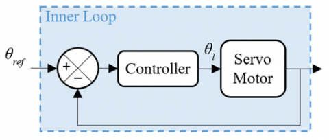
As mentioned in the previous section that the system is asymmetric and decoupled, then one axis is sufficient to study its behavior. The x-axis which is servo2 based unit is chosen to design the controller. Figure 4 depicts the control structure in two loops outer and inner respectively the ball position loop and servo2-based unit loop, which calculates the required voltage to track the load at the appropriate angle.
Figure 4. Control loop structure
Three techniques were chosen in this assessment in term of dynamic range and ability to yield the system to satisfy the design specifications which are found challenge in literature survey, Linear quadratic regulator (LQR) is a popular method for optimal, resilient and robust control of dynamic systems in mechatronics. It minimizes a cost function that weighs control effort against deviation from the target state. The use of a full state feedback and proportional derivative controller to 2-DOF ball balancer model can incorporate the design specification directly to synthetize the feedback gain in the close loop.
3.1 Design specifications
The required parameters of the design controllers are:
1. Settling time $\leq 3$ sec.
2. Percentage Overshoot $P_o \leq 10 \%$.
3. Steady state error $\mathrm{e}_{\mathrm{rr}} \leq 5 \mathrm{~mm}$.
3.1.1 Infinite horizon linear quadratic regulation
Linear quadratic regulator (LQR) uses the linear dynamic continuous or discrete time of a system call linear state space form and the cost function is a quadratic form. LQR is an ideal multivariable feedback control strategy that minimizes the excursion in a system's state trajectories while requiring the least amount of controller effort. An LQR controller's behavior is determined by two parameters: the state and control weighting matrices. These two matrices are the primary design factors that must be chosen by the designer and have a significant impact on the success of the LQR controller synthesis [31]. It is well known that the optimal LQR controller is resilient by nature, robust [32]. LQR is efficient and applied in many robotics system, aerospace system, mechanical and electrical system.
The design of the LQR controller required two criteria on the system states:
1. The controllability
$C=\operatorname{rank}\left[\begin{array}{lllll}\mathrm{B} & \mathrm{AB} & \mathrm{A}^2 \mathrm{~B} & \ldots, \quad \mathrm{A}^{\mathrm{n}-1} \mathrm{~B}\end{array}\right]=\mathrm{n}$ (14)
$C=\operatorname{det}\left(\left[\begin{array}{cc}0 & 1.0873 \\ 1.0873 & 0\end{array}\right]\right)=-1.1822 \neq 0$
If the two rows or columns are not independent and the determinant is different than zero, then the system is controllable.
2. The observability
$\mathrm{O}=\operatorname{Rank}\left[\begin{array}{c}\mathrm{CA} \\ \mathrm{CA}^2 \\ \mathrm{CA}^3 \\ \vdots \\ C A^{\mathrm{n}-1}\end{array}\right]=\mathrm{n}$ (15)
$0=\operatorname{det}\left(\left[\begin{array}{ll}0 & 1 \\ 1 & 0\end{array}\right]\right)=-1 \neq 0$
If the determinant of the observability matrix is different than zero then: The system is said Observable.
Let x be the solution of the system (12) and the cost function be:
$\mathrm{J}(\mathrm{x}, \mathrm{u})=\int_0^{\infty}\left(\mathrm{x}^{\mathrm{T}}(\mathrm{t}) \mathrm{Qx}(\mathrm{t})+\mathrm{u}^{\mathrm{T}}(\mathrm{k}) \mathrm{Ru}(\mathrm{k})\right) d \mathrm{t}$ (16)
Q is a symmetric, positive semidefinite (N Ⅹ N) matrix, and R is symmetric, positive definite (M Ⅹ M) matrix. The matrices Q, and R are tuning parameters for meeting design requirements. Whereas Q penalizes delayed responses and overshoots, R penalizes the input of the system.
Proposition 1: Assume that $\mathrm{Q}$ is 0 and $\mathrm{R}$ is 0 and that (A, $B)$ is stabilizable $(\mathrm{Q}, \mathrm{A})$ is detectable. The ideal $\mathrm{LQR}$ policy is given by the equation $\mathrm{u}(\mathrm{t})=\mathrm{kx}(\mathrm{t})$, where $K=-R^{-1} B^T P$ and $X \geq 0$ is the sole stabilizing solution to the algebraic Riccati equation [32].
In the case of the system (12), the control law is express $u(t)=-R^{-1} B^T P x(t)$, with $P$ satisfied the Algebraic Riccati Eq. (ARE) below:
$\mathrm{PA}+\mathrm{A}^{\mathrm{T}} \mathrm{P}-\mathrm{PBR}^{-1} \mathrm{~B}^{\mathrm{T}} \mathrm{P}+\mathrm{Q}=0$ (17)
Weighting matrix $\mathrm{Q}$ is obtained by trial-and-error within the value of: $Q=\left[\begin{array}{cc}50 & 1 \\ 0 & 0.1\end{array}\right]$ and $\mathrm{R}=1$ with feedback gains $\mathrm{K}=\left[\begin{array}{ll}7.07 & 3.62\end{array}\right]^T$.
3.1.2 PD controller design
The conventional controller PD has a significant range of use in industries [33] because of its simplicity to design but also its easier real implementation. The Figure 5 below shows the structure of the control in a double loop outer and inner loop respectively, the outer loop is the ball position under PD controller and the inner is the servo2 x angular displacement under proportional controller.
Figure 5. Structure loop of PD controller
The model, transfer function of the servo2 based unit and the ball position used in this part of the work is given by the study [34].
$\frac{\theta_l(s)}{V_m(s)}=\frac{K}{s(\tau s+1)}$ (18)
The transfer function that described the ball position is:
$\frac{X_b(s)}{\theta_l(s)}=\frac{K_{b b}}{s^2}$ (19)
By deriving the expression of the desired angular displacement with respect to the reference signal in the ball position control loop, the expression below is gotten:
$\theta_{\mathrm{d}}(\mathrm{s})=\mathrm{K}_{\mathrm{pb}}\left(\mathrm{X}_{\mathrm{r}}(\mathrm{s})-\mathrm{X}_{\mathrm{b}}(\mathrm{s})\right)-\mathrm{K}_{\mathrm{db}} \mathrm{SX} \mathrm{b}(\mathrm{s})$ (20)
Assuming that the inner loop is ideal, which means that the desired angular displacement is equal to the angular computed by the servo2 load.
$\theta_{\mathrm{d}}(\mathrm{s})=\theta_l(s)$ (21)
Replacing Eq. (20) in (19), and then rearranging it, the second order transfer function of the ball position is obtained.
$\frac{X_b(s)}{X_r(s)}=\frac{K_{b b} K_{p b}}{S^2+K_{b b} K_{d b} s+K_{b b} K_{p b}}$ (22)
The gain of the proportional derivative controller was synthesized by comparing the transfer function (22) to (23) shown below, damping ratio and natural frequency were determined from Eqs. (25) and (24).
$F(s)=\frac{w_n{ }^2}{\mathrm{~S}^2+2 \varepsilon \mathrm{W}_{\mathrm{n}} \mathrm{s}+\mathrm{w}_{\mathrm{n}}{ }^2}$ (23)
$t_s=\frac{\left.\ln \sqrt{(1}-\varepsilon^2\right)}{\varepsilon w_n}$ (24)
$P_o=100 \mathrm{e}^{-\frac{\pi \varepsilon}{\sqrt{\left(1-\varepsilon^2\right)}}}$ (25)
3.1.3 Full state feedback design
As state in the subsection 3.1.1 the system is full rank, controllable and observable. The design problem known as control input is:
$\theta_{\mathrm{l}}(\mathrm{t})=-\mathrm{KX}(\mathrm{t})$ (26)
By substituting the control law in the system (12), end up the close loop of the system in the form of $\Delta=(\mathrm{A}-\mathrm{BK})$:
$\left[\begin{array}{l}\dot{\mathrm{x}}_1(\mathrm{t}) \\ \dot{\mathrm{x}}_2(\mathrm{t})\end{array}\right]=\left[\begin{array}{cc}0 & 1 \\ -K K_{-b b} & -K K_{-b b}\end{array}\right]\left[\begin{array}{l}\mathrm{x}_1(\mathrm{t}) \\ \mathrm{x}_2(\mathrm{t})\end{array}\right]$ (27)
The design of feedback gains is obtained by Cayley Hamilton Theorem:
$\Delta^2+\beta_1 \Delta+\beta_2 I=0$ (28)
Determined the close loop characteristics polynomial $\rho(\Delta)$ from the expression above:
$\rho(\Delta)=A B K+B K \Delta+\beta_1 B K$ (29)
$\rho(\Delta)=\left[\begin{array}{ll}\mathrm{B} & \mathrm{AB}\end{array}\right]\left[\begin{array}{c}\beta_1 \mathrm{~K}+\mathrm{K} \Delta \\ \mathrm{K}\end{array}\right]$ (30)
where, $C=\left[\begin{array}{ll}\mathrm{B} & \mathrm{AB}\end{array}\right]$ is the controllabillity matrix non singular.
Multiplying both side the expression (30) by $\left[\begin{array}{ll}0 & 1\end{array}\right] \mathrm{C}^{-1}$ we end up getting the feedbak gains:
$K=\left[\begin{array}{ll}0 & 1\end{array}\right] 0^{-1} \rho(\Delta)$ (31)
The feedback gain found for full sate feedback controller is:
$K=\left[\begin{array}{ll}9.54 & 4.05\end{array}\right]^T$
3.2 Inner loop controller
The inner loop is the servo2 based unit angular position control under the proportional controller. The error from desired angular position computed from the ball position and inner loop is corrected by adjusting empirically the gain Kp which was satisfied with a value of 14. Figure 6 shows the servo2 based unit controller in a closed loop.
Figure 6. Close loop of the servo2
Simulation and real implementation of the three controllers with the help of hardware, 2-DOF ball balancer with two servo2 based unit along x and y axis, a camera attached it, 2X amplifiers, Data acquisition card all Quanser materials and HP laptop. MATLAB/Simulink integrates QUARC software. The Figure 7 shows the materials used during experiment conduction.
Figure 7. Wiring and experiment materials
4.1 Simulation and experiment results
The comparison that has been conducted in this work was mainly focused on the best choice of the model that captured closely the system dynamic on one hand but also the performance of the control technique to achieve the best position tracking of the ball with minimum steady state error, less percentage overshoot, less peak time and settling time in another hand.
The transient and steady-state responses are crucial in characterizing the system's behavior. They also facilitate informed decisions regarding the selection of effective and performant controller. This last yield the system to track the reference but also to have a minimum angular displacement of servo2 x, with minimum energy consumption (Voltage).
The stability of 2-DOF ball balancer system is analysed with Lyapunov criteria, since the $R>0$ and $Q \geq 0, Q=C^T * C$ and the couple $(A, B)$ is controllable and $(A, C)$ is observable, there exists a unique solution to the algebraic Riccati equation and the optimal closed loop system $\dot{x}=(A-B K) x$, where $K=-R^{-1} B^T P$, with the negative real part of the eigenvalues. The Lyapunov s' stability criterion.
$V(x)=x^T P x$ (32)
where, $P>0$ is the solution of the Riccati Eq. (17).
Taken the derivative of the Lyapunov of Eq. (32)
$\dot{V}(x)=2 x^T P \dot{x}$ (33)
$\dot{V}(x)=x^T P(A-B K) x+x^T(A-B K)^T P x<0$ (34)
Eq. (34) has to be demonstrated.
Taking the algebraic Riccati Eq. (17) and manipulating it, the following equation is derived:
$P(A-B K)+(A-B K)^T P=-K^T B^T P-Q$ (35)
Eqs. (33) to (34), can be written as:
$x^T P(A-B K) x+x^T(A-B K)^T P x=-\left(K^T B^T P+\right.Q)$ (36)
With $K>0 ; Q \geq 0 ; B>0 ; P>0$.
$\left(K^T B^T P+Q\right)>0$
$\dot{V}(x)=-x^T\left(K^T B^T P+Q\right) x<0$
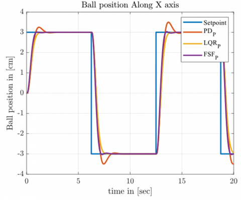
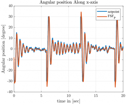
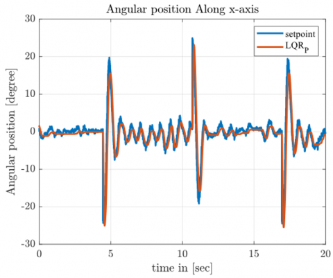
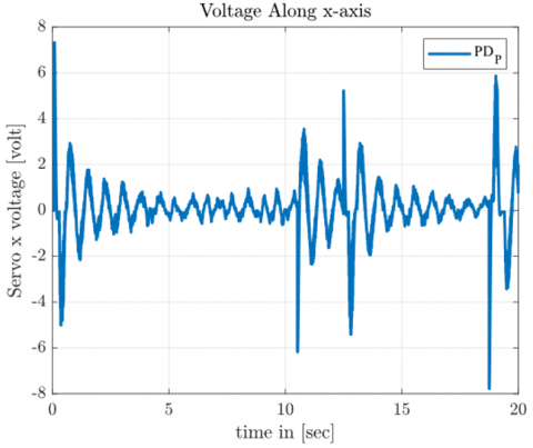
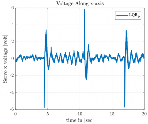
Hence the close loop of LQR in the form of (A-BK) is globally asymptotically stable. The three figures below depicted the simulation results: Figure 8 shows the ball position, Figure 9 shows the angle of the central beam-plate system and Figure 10 shows the voltage consumed by the servo2 based unit along the x-axis. Figure 11 depicted the experiment results of the ball position, Figures 12-14 show the angular position and Figures 15-17 depict the voltages of three controllers respectively PD_P, LQR_P and FSF_P.
Figure 8. Simulation results of LQR, PD and FSF
Figure 9. Angular position of servo motor X
Figure 10. Voltage of servo X
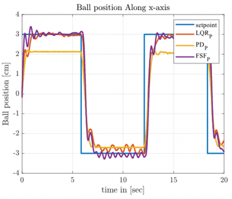
Figure 11. Experiment of ball position with LQR_P, FSF_P and PD_P
Figure 12. Angular position along x axis PDp
Figure 13. Angular position along x axis FSFp
Figure 14. Angular position along x axis LQRp
Figure 15. Voltage of servo X PDp
Figure 16. Voltage of servo X LQRp
Figure 17. Voltage of servo X FSFp
4.2 Simulation and experiment results discussion
The comparison made during Simulation and real Implementation of the three controllers is based on the time domain and steady state error. The reference signal is chosen to be between -3 cm and +3 cm as is pose as challenge in literature survey by many researchers. During this study and analysis, it is found from Tables 1 and 2 that LQR_P has the lowest steady state error and lowest percentage overshoot both from the simulation and experiment respectively 1.15e-10, 0.064 cm and 0, 3.96% compared to PD_P and FSF_P. Full state feedback based proportional has the greater settling time from the experiment of 5.75sec and lowest from the simulation 0.82 sec compared to other controllers. Full state feedback based proportional and proportional derivative based proportional have smallest peak time for simulation and experiment both as show in Tables 1 and 2.
Table 1. Simulation comparative assessment of controllers
|
Controllers |
Settling Time ts (sec) |
Peak Time tp (sec) |
Overshoot % |
Steady State Error (cm) |
|
PD_P |
1.71 |
1.19 |
8.25 |
1.00e-06 |
|
FSF_P |
0.82 |
1.02 |
0.38 |
2.55e-10 |
|
LQR_P |
1.12 |
2.88 |
0 |
1.15e-10 |
Table 2. Experiment comparative assessment of controllers
|
Controllers |
Settling Time ts (sec) |
Peak Time tp (sec) |
Overshoot % |
Steady State Error (cm) |
|
PD_P |
0.70 |
0.55 |
4.76 |
0.88 |
|
FSF_P |
5.75 |
0.85 |
8.02 |
0.39 |
|
LQR_P |
3.83 |
1.97 |
3.96 |
0.064 |
The angular displacement of servo x with respect to PD_P and FSF_P controllers exceeded the bound of 30 degrees, but also the high voltage, between -8 to 8 and -10 to 10 compared to LQR_P with a minimum and maximum angular position of -25 to 25 degrees and a voltage of -6 to 6v. then compare all approaches to our given specifications, only the linear quadratic regulator based proportional satisfied 66.66% with good trajectory tracking and minimum steady state error. Even if the settling time was not satisfied but it ranges. Linear quadratic regulator based proportional have good tracking trajectory compared to the rest of control techniques investigated in this study.
In conclusion, we delved into the model design of a 2-DOF ball balancer system, characterized by its electromechanical nature, under actuation, instability, and pronounced nonlinearity. We rigorously tested three control techniques: LQR_P, FSF_P, and PD_P. These were employed to establish a correlation between the real system and the mathematical model developed herein. Additionally, their performance and efficacy were evaluated through time-domain analysis. Both simulations and experiments were conducted, revealing that the Linear Quadratic Regulator based proportional control (LQR_P) satisfied the steady state error and percentage overshoot even if it is failed on settling time. Although Full State Feedback based proportional (FSF_P) control exhibited commendable performance, it was surpassed by Proportional Derivative based proportional (PD_P) control. FSF_P and PD_P are not optimal control and non-robust controller to uncertainties such as variation of the light and wind. Notably, LQR_P is an optimal, robust controller, integrated with image-based servoing in the feedback system, demonstrated superior effectiveness in trajectory tracking. Tuning the weighting matrices Q and R by optimal control such as PSO, GA etc. to avoid trial and error can be consided as future work.
[1] Tian, Y., Bai, M., Su, J. (2006). A non-linear switching controller for ball and plate system. International Journal of Modelling, Identification and Control, 1(3): 177-182. https://doi.org/10.1504/IJMIC.2006.011940
[2] Ker, C.C., Lin, C.E., Wang, R.T. (2007). Tracking and balance control of ball and plate system. Journal of the Chinese institute of engineers, 30(3): 459-470. https://doi.org/10.1080/02533839.2007.9671274
[3] Mochizuki, S., Ichihara, H. (2013). I-PD controller design based on generalized KYP lemma for ball and plate system. In 2013 European control conference (ECC), Zurich, Switzerland, pp. 2855-2860. https://doi.org/10.23919/ecc.2013.6669269
[4] Sun, S.Q., Li, L. (2012). The study of ball and plate system based on non-linear PID. Applied Mechanics and Materials, 187: 134-137. https://doi.org/10.4028/www.scientific.net/AMM.187.134
[5] Wang, H., Tian, Y., Sui, Z., Zhang, X., Ding, C. (2007). Tracking control of ball and plate system with a double feedback loop structure. In 2007 International Conference on Mechatronics and Automation, Harbin, China, pp. 1114-1119. https://doi.org/10.1109/ICMA.2007.4303704
[6] Shiratori, T., Zanma, T., Liu, K. (2014). Optimal quantization feedback control with variable discrete quantizer. In 2014 IEEE 13th International Workshop on Advanced Motion Control (AMC), Yokohama, Japan, pp. 116-121. https://doi.org/10.1109/AMC.2014.6823267
[7] Subramanian, R.G., Elumalai, V.K., Karuppusamy, S., Canchi, V.K. (2017). Uniform ultimate bounded robust model reference adaptive PID control scheme for visual servoing. Journal of the Franklin Institute, 354(4): 1741-1758. https://doi.org/10.1016/j.jfranklin.2016.12.001
[8] Kaan, C., Başçi, A. (2017). Position control of a ball & beam experimental setup based on sliding mode controller. International Journal of Applied Mathematics Electronics and Computers, 1: 29-35. https://doi.org/10.18100/ijamec.2017SpecialIssue30467
[9] Ma, J., Tao, H., Huang, J. (2021). Observer integrated backstepping control for a ball and plate system. International Journal of Dynamics and Control, 9: 141-148. https://doi.org/10.1007/s40435-020-00629-8
[10] Singh, R., Bhushan, B. (2020). Real-time control of ball balancer using neural integrated fuzzy controller. Artificial Intelligence Review, 53(1): 351-368. https://doi.org/10.1007/s10462-018-9658-7
[11] Pasha, J.F., Mija, S.J. (2019). Discrete Laguerre based MPC for constrained asymptotic stabilization of 4 DOF ball balancer systems. In 2019 IEEE 5th International Conference on Mechatronics System and Robots (ICMSR), Singapore, pp. 76-80. https://doi.org/10.1109/ICMSR.2019.8835465
[12] Singh, R., Bhushan, B. (2021). Improved ant colony optimization for achieving self-balancing and position control for balancer systems. Journal of Ambient Intelligence and Humanized Computing, 12: 8339-8356. https://doi.org/10.1007/s12652-020-02566-y
[13] Singh, R., Bhushan, B. (2022). Adaptive control using stochastic approach for unknown but bounded disturbances and its application in balancing control. Asian Journal of Control, 24(3): 1304-1320. https://doi.org/10.1002/asjc.2586
[14] Zarzycki, K., Ławryńczuk, M. (2021). Fast real-time model predictive control for a ball-on-plate process. Sensors, 21(12): 3959. https://doi.org/10.3390/s21123959
[15] Ali, H.I., Jassim, H.M., Hasan, A.F. (2019). Optimal nonlinear model reference controller design for ball and plate system. Arabian Journal for Science and Engineering, 44(8): 6757-6768. https://doi.org/10.1007/s13369-018-3616-1
[16] Dong, X., Zhang, Z., Tao, J. (2009). Design of fuzzy neural network controller optimized by GA for ball and plate system. In 2009 Sixth International Conference on Fuzzy Systems and Knowledge Discovery, Tianjin, China, pp. 81-85. https://doi.org/10.1109/FSKD.2009.710
[17] Wang, Y., Jin, Q., Zhang, R. (2017). Improved fuzzy PID controller design using predictive functional control structure. ISA Transactions, 71: 354-363. https://doi.org/10.1016/j.isatra.2017.09.005
[18] Mohammadi, A., Ryu, J.C. (2020). Neural network-based PID compensation for nonlinear systems: Ball-on-plate example. International Journal of Dynamics and Control, 8(1): 178-188. https://doi.org/10.1007/s40435-018-0480-5
[19] Wang, H., Tian, Y., Fu, S., Sui, Z. (2008). Nonlinear control for output regulation of ball and plate system. In 2008 27th Chinese Control Conference, Kunming, China, pp. 382-387. https://doi.org/10.1109/CHICC.2008.4605473
[20] Wang, Y., Sun, M., Wang, Z., Liu, Z., Chen, Z. (2014). A novel disturbance-observer based friction compensation scheme for ball and plate system. ISA Transactions, 53(2): 671-678. https://doi.org/10.1016/j.isatra.2013.11.011
[21] Beckerleg, M., Hogg, R. (2016). Evolving a lookup table based motion controller for a ball-plate system with fault tolerant capabilites. In 2016 IEEE 14th International Workshop on Advanced Motion Control (AMC), pp. 257-262. https://doi.org/10.1109/AMC.2016.7496360
[22] Fan, J., Han, M. (2012). Nonliear model predictive control of ball-plate system based on gaussian particle swarm optimization. In 2012 IEEE Congress on Evolutionary Computation, pp. 1-6. https://doi.org/10.1109/CEC.2012.6252950
[23] Okafor, E., Udekwe, D., Ibrahim, Y., Bashir Mu'azu, M., Okafor, E.G. (2021). Heuristic and deep reinforcement learning-based PID control of trajectory tracking in a ball-and-plate system. Journal of Information and Telecommunication, 5(2): 179-196. https://doi.org/10.1080/24751839.2020.1833137
[24] Pattanapong, Y., Deelertpaiboon, C. (2013). Ball and plate position control based on fuzzy logic with adaptive integral control action. In 2013 IEEE International Conference on Mechatronics and Automation, pp. 1513-1517. https://doi.org/10.1109/ICMA.2013.6618138
[25] Bang, H., Lee, Y.S. (2018). Implementation of a ball and plate control system using sliding mode control. IEEE Access, 6: 32401-32408. https://doi.org/10.1109/ACCESS.2018.2838544
[26] Moreno-Armendáriz, M.A., Pérez-Olvera, C.A., Rodríguez, F.O., Rubio, E. (2010). Indirect hierarchical FCMAC control for the ball and plate system. Neurocomputing, 73(13-15): 2454-2463. https://doi.org/10.1016/j.neucom.2010.03.023
[27] Hesar, M.E., Masouleh, M.T., Kalhor, A., Menhaj, M.B., Kashi, N. (2014). Ball tracking with a 2-DOF spherical parallel robot based on visual servoing controllers. In 2014 Second RSI/ISM International Conference on Robotics and Mechatronics (ICRoM), Tehran, Iran, pp. 292-297. https://doi.org/10.1109/ICRoM.2014.6990916
[28] Roy, P., Das, A., Roy, B.K. (2018). Cascaded fractional order sliding mode control for trajectory control of a ball and plate system. Transactions of the Institute of Measurement and Control, 40(3): 701-711. https://doi.org/10.1177/0142331216663826
[29] Pasha, J.F., Mija, S.J. (2019). Asymptotic stabilization and trajectory tracking of 4 DoF ball balancer using LQR. In TENCON 2019-2019 IEEE Region 10 Conference (TENCON), pp. 1411-1415. https://doi.org/10.1109/TENCON.2019.8929327
[30] Kostamo, J., Hyotyniemi, H., Kuosmanen, P. (2005). Ball balancing system: An educational device for demonstrating optimal control. In 2005 International Symposium on Computational Intelligence in Robotics and Automation, Espoo, Finland, pp. 379-384. https://doi.org/10.1109/cira.2005.1554306
[31] Hassani, K., Lee, W.S. (2014). Optimal tuning of linear quadratic regulators using quantum particle swarm optimization. In Proceedings of the International Conference on Control, Dynamic Systems, and Robotics (CDSR’14), Ottawa, Ontario, Canada, pp. 1-8.
[32] Kashyap, M., Lessard, L. (2023). Guaranteed stability margins for decentralized linear quadratic regulators. IEEE Control Systems Letters, 7: 1778-1782. https://doi.org/10.1109/LCSYS.2023.3280868
[33] Adel, T., Abdelkader, C. (2013). A particle swarm Optimization approach for optimum design of PID controller for nonlinear systems. In 2013 International Conference on Electrical Engineering and Software Applications, pp. 1-4. https://doi.org/10.1109/ICEESA.2013.6578478
[34] Motion, R., Plant, S. (2015). Rotary Experiment #17: 2D Ball Balancer. https://nps.edu/documents/105873337/0/56%20-%202D%20Ball%20Balancer%20Control%20-%20Instructor%20Manual.pdf/709c97d2-0fae-426c-9e2a-4b36e8411edf.