Ilyes Dahnoun*![]() | Amor Bourek
| Amor Bourek![]() | Abdelkarim Ammar
| Abdelkarim Ammar![]() | Oussama Belaroussi
| Oussama Belaroussi![]()
© 2024 The authors. This article is published by IIETA and is licensed under the CC BY 4.0 license (http://creativecommons.org/licenses/by/4.0/).
OPEN ACCESS
Improving tracking performance in speed controllers for permanent-magnet synchronous motor (PMSM) drive systems is critical due to internal challenges such as parameter variations, model uncertainty, and external disturbances like load changes. This paper proposes a new method that combines sensorless model predictive control (MPC) with active disturbance rejection control (ADRC), employing an extended state observer (ESO) as a key component of the ADRC. Notably, the proposed ADRC-MPC control integrates the advantages of MPC, such as good time response, high robustness against load variation, and a low effect of parameter variation in comparison to conventional control methods like field-oriented control (FOC). The ADRC-MPC reduces torque and flux ripples and also reduces torque and flux irregularities as well as current harmonics, which presents a major drawback in direct torque control (DTC). The proposed control with finite set model predictive control (FS-MPC) eliminates the PWM modulation and the complexity of continuous control set model predictive control (CCS-MPC). In the outer loop, the ADRC-MPC and the ESO present a very good solution. It presents a lower processing requirement than other controllers, especially the fuzzy logic controller (FLC), and also presents a consistent dynamic behavior across the entire operating range, contrary to the PID. The ADRC with ESO presents a promising solution to these challenges. The effectiveness of the proposed method is demonstrated through numerical simulations using MATLAB/Simulink software and experiments on a 3-kW surface-mounted PMSM drive system. both simulation and experimental results under different conditions show the effectiveness of the proposed approach.
active disturbance rejection control (ADRC), extended state observer (ESO), model predictive control (MPC), model reference adaptive system (MRAS), PMSM
PMSMs have extensive use across diverse sectors such as machine tools, robotics, automotive, healthcare, aviation, and aeronautics [1, 2]. When compared to other kinds of motors, the PMSM has shown exceptional performance in several aspects including high efficiency, absence of excitation windings, compact dimensions, high power and torque density, and a reduced volume [3]. FOC is widely used as the predominant control approach in drives for PMSM due to its exceptional steady-state performance. This approach utilizes coordinate transformation to effectively segregate the stator current into two distinct components: a torque current component and an excitation current component. Furthermore, this methodology incorporates the implementation of pulse width modulation techniques. DTC has a faster dynamic reaction in comparison to FOC. The fundamental concept behind DTC is the selection of the most suitable voltage space vector from a predetermined switching table. This selection is made with the objective of minimising the discrepancy between the stator flux and electromagnetic torque [4]. The accurate calibration of the internal loop is essential in order to provide smooth operation throughout a broad spectrum of speeds. By using DTC, the need for a current loop and the accompanying tuning process is obviated. Furthermore, the use of a preset switching table obviates the need of the PWM block, since it provides the appropriate voltage vector. Consequently, a fast reaction is achieved by a simple structure. Nevertheless, the primary limitations of DTC include substantial variations in torque and flux, alongside undesirable acoustic emissions [5, 6]. PID controllers are commonly utilised in linear time-invariant systems due to their straightforward design, reliable steady-state accuracy, and exceptional stability. These systems often face challenges arising from various factors, including unpredictable external load disturbances, inconsistent internal friction, and the intricate impacts of non-linear magnetic fields [7]. In the study conducted by the authors, the PID controller used in reference [8] was substituted with a Takagi-Sugeno fuzzy logic controller. This modification was made in order to compensate for load uncertainties and enhance the system's reaction time. On the contrary, the use of a substantial quantity of fuzzy sets is needed in order to achieve a high-performance fuzzy controller, resulting in an augmented computational load. In order to address the aforementioned issues and enhance driver dynamic performance, there has been significant interest in the adoption of novel control methodologies this paper present an new approach using ADRC. ADRC is a potential approach for improving the robustness of control systems. This approach excels in actively estimating and rejecting total disturbances, both known and unknown. This approach is very resistant to disturbances as it doesn't require an exact system model, MPC and ADRC. MPC has a higher bandwidth in comparison to the conventional PI controller approach. The present controller has been used in previous studies [9, 10]. The use of ADRC has become more attractive in several industrial sectors, including motion control, power electronics, and robotic systems. This is mostly due to ADRC's capacity to effectively manage uncertainties, exhibit robustness, and provide advantages that are not heavily reliant on the specific plant model [11]. This work proposes model predictive direct torque control using an ADRC-MPC to address issues with huge torque and speed ripples and control system resilience.
The efficacy of the suggested control method is shown via simulation using MATLAB/Simulink and experimental verification through real-time implementation with the dSpace 1104 acquisition card inside the Control Desk environment. The paper is structured in the following manner. The first presentation of the system's model, which includes the motor and load, is conducted using Park's coordinate system (d, q). Section III discusses the mathematical approach of the Load Disturbance Observer (DOB), while section IV presents the model reference adaptive system as an observer of the motor speed. In section V, the simulation results obtained using MATLAB/Simulink are presented, including a comparison between the proposed technique and PID. Subsequently, the ensuing section will delve into the discourse of the experimental findings pertaining to the suggested control technique, namely ADRC-MPC. Ultimately, the conclusion will be presented.
2.1 Motor continuous state-space model and state variables for MPC
In order to enhance the ease of analysis while preserving control performance, some assumptions are made about the electromagnetic interaction between the stator and rotor of a PMSM that are coupled via a magnetic field in an air gap. The following assumptions are:
The disregard of iron saturation in the stator leads to an underestimation of the iron loss, which constitutes a significant component of the overall losses in PMSMs. Hence, achieving highly efficient motors requires a thorough understanding of the motor's iron loss process and meticulous calculations. The iron loss is contingent upon the characteristics of the flux waveform, including its frequency and amplitude. During full load circumstances, the motors experience three different states of the magnetic field: unsaturated, saturated, and locally severely saturated. Varying levels of saturation will impact the magnetization process in silicon steel, resulting in varying degrees of iron loss. This issue has been addressed in reference [12]. The impact of eddy currents and hysteresis is not accounted for in the analysis. Various additional terms for flux density are used to offset the increased hysteresis and eddy current loss resulting from the non-linear behavior of the magnetic chain in the silicon steel sheet and the higher harmonic magnetic field. This issue has been extensively discussed in reference [13]. It is widely assumed that the three phase windings of the stator exhibit symmetrical characteristics [14]. Subsequently, The first step in the development of a MPC framework is the establishment of a discrete-time model for the system. The category of systems that may be represented by a linear model with constraints is particularly well-suited for the implementation of MPC. This is because a significant portion of the optimisation process can be performed offline in such cases. In order to effectively follow the linear model, it is essential to make appropriate decisions about the state variables. $\frac{d x(t)}{d t}=$ $g(x(t), u(t))$ can be used to denote the state space representation for the PMSM, where the input signal is the 2-D voltage vector $u=\left[u_d u_q\right]^T$ and the state vector $x=\left[i_d i_q \omega\right]^T$ [15-18]. In light of this decision, the motor's continuous state-space model is as follows:
$\begin{gathered}\frac{d}{d t}\left[\begin{array}{cc}i_d(t) \\ i_q(t) \\ \omega(t)\end{array}\right] ={\left[\begin{array}{ccc}-\frac{R}{L_d} & \frac{L_q}{L_d} \omega(t) & 0 \\ -\frac{L_d}{L_q} \omega(t) & -\frac{R}{L_q} & -\frac{1}{L_q} \psi_{p m} \\ 0 & \frac{1.5 p^2}{J} \psi_{p m} & -\frac{B m}{J}\end{array}\right]\left[\begin{array}{l}i_d(t) \\ i_q(t) \\ \omega(t)\end{array}\right]} +\left[\begin{array}{ccc}\frac{1}{L_d} & 0 & 0 \\ 0 & \frac{1}{L_q} & 0 \\ 0 & 0 & -\frac{p}{J}\end{array}\right]\left[\begin{array}{l}u_d(t) \\ u_q(t) \\ T_L(t)\end{array}\right]\end{gathered}$ (1)
2.2 Motor model discretization
By using a discrete model of the motor and its drive, one may forecast the current at sampling time k+1 by leveraging the observed position, speed, and currents at sampling time k. The discrete time model obtained by applying forward Euler discretization theory to Eq. (1) is represented as a discrete time model [17].
$x(k+1)=A.x(k)+B. u(k)$ (2)
where, $\omega$ and $J_{e q}$ are, respectively, the electrical angular velocity of the rotor, and the equivalent inertia of the motor and the load.
$\begin{aligned} & {\left[\begin{array}{c}i_d(k+1) \\ i_q(k+1) \\ \omega(k+1)\end{array}\right]} =\left[\begin{array}{ccc}1-\frac{R}{L_d} T & \frac{L_q \omega(k)}{L_d} T & 0 \\ 0 & 1-\frac{R}{L_q} T & -\frac{\left(L_d i_d(k)+\psi_{p m}\right)}{L_q} T \\ 0 & \frac{1.5 p^2 \psi_{p m}}{J} T & 1-\frac{B m}{J} T\end{array}\right] \\ & {\left[\begin{array}{c}i_d(k) \\ i_q(k) \\ \omega(k)\end{array}\right]+\left[\begin{array}{ccc}\frac{1}{L_d} T & 0 & 0 \\ 0 & \frac{1}{L_q} T & 0 \\ 0 & 0 & -\frac{p}{J} T\end{array}\right]\left[\begin{array}{c}u_d(k) \\ u_q(k) \\ T_L(k)\end{array}\right]} \\ & \end{aligned}$ (3)
The variables udand uq denote the d-q axes voltages, while id and iq represent the d-q axes currents. Additionally, $\psi_{p m}$ signifies the permanent magnet flux linkage, and R designates the winding resistance. Given the utilization of a surface permanent magnet synchronous motor (SPMSM) in this study, it is pertinent to note that the cross-axes and straight-axes inductances are equitably matched, denoted as L=Ld=Lq. The formulation outlined in Eq. (1) dictates the current state at the subsequent time step [id(k+1) and iq(k+1)] through the application of the forward Euler discretization scheme, as expounded in references [18, 19]:
$\left\{\begin{array}{c}i_d(k+1)=\left(1-\frac{T R}{L}\right) \cdot i_d(k)+T \omega_e i_q(k) +\frac{T}{L} u_d(k) \\ i_q(k+1)=\left(1-\frac{T R}{L}\right) \cdot i_q(k)-T \omega_e i_d(k)+\frac{T}{L} u_q(k) -\frac{T \omega_e \psi_{p m}}{L}\end{array}\right.$ (4)
2.3 Voltage source inverter
A two-level voltage source inverter (VSI) fed PMSM in this study. The following equation produces the voltage vector:
$V_s=\sqrt{\frac{2}{3}} V_{D C}\left[S_a+S_b e^{j \frac{2 \pi}{3}}+S_c e^{j \frac{4 \pi}{3}}\right]$ (5)
where, $V_{D C}$ denote the $\mathrm{DC}$ link voltage. Control of the inverter is based on logic values $S_i$, where, $S_i=1, T_i$ is ON and $\bar{T}_i$ is OFF. $S_i=0, T_i$ is OFF and $\bar{T}_i$ is ON, $i=a, b, c$.
A total of eight distinct places might potentially arise as a consequence of various combinations of the switching states. The two remaining vectors have a magnitude of zero, whereas the remaining six vectors are active.
2.4 Cost function design
The main objectives of the predictive current control methodology are to effectively follow the torque current reference and limit the magnitude of the current [17]. The above listed goals may be articulated by using a cost function.The cost function used in MPC approach entails the evaluation of projected values in relation to reference values.
$\begin{gathered}g=\left(i_d^p(k+1)\right)^2+\left(i_q^*-i_q^p(k+1)\right)^2+\hat{f}\left(i_d^p(k+1), i_q^p(k+1)\right)\end{gathered}$ (6)
The primary function of the first component is to reduce reactive power, hence enabling smoother operation. The second term refers to the aim of precisely monitoring the electrical current that is accountable for producing torque. The last element in the equation reflects a non-linear function that imposes limitations on the amplitude of the stator currents. The function f is characterised by its complexity, mostly attributed to the incorporation of constraints on the maximum stator current, which rigorously limit the range of acceptable values.
$\hat{f}\left(i_d^p, i_q^p\right) \triangleq\left\{\begin{array}{l}\infty \,\,if \,\left|i_q^p\right|>\hat{i}_q \,\, or \,\left|i_d^p\right|>\hat{i}_d \\ 0 \,\,if \,\left|i_q^p\right|=\hat{i}_q \,\,and\, \left|i_d^p\right|=\hat{i}_d\end{array}\right.$ (7)
The components of the voltage vectors are projected by using the known rotor position for each potential switching configuration throughout the three phases. The determination of the stator current components is thereafter based on many factors, including the predicted voltage vectors, the observed stator currents ($\hat{l}$), the intrinsic features of the machine and the sampling interval (T). The implementation of stator current management is crucial for ensuring the effective execution of safety protocols in order to mitigate overcurrent problems across various operational velocities. Furthermore, the goal function is enhanced by including a variable represented by "n" to decrease the frequency of power switch toggling. The careful examination of inverter dead-time is of utmost importance to mitigate the occurrence of short-circuit problems that may occur during commutation instances. Furthermore, a mechanism is included to provide compensation for the voltage drop that arises as a consequence of the dead-time. The highest attainable value of the objective function has been documented [17].
The disruptions encountered by PMSM systems may be classified as lumped disturbances, including both internal and external influences. There are two primary disruptions in the functioning of a PMSM: external disturbances, which include changes in load and reference signals, and inertial disturbances, which involve changes in parameters and unmodeled dynamics. The system disturbance primarily has three components: (1) load-induced disturbance, (2) speed-induced disturbance, and (3) reference speed-induced disturbance. These disturbances include changes in load torque as well as dynamics that have not been accurately anticipated. Omitting the necessary feedforward compensation control mechanism to counteract these disturbances will negatively affect the performance of the closed-loop system. Before proceeding, it is essential to first conduct an evaluation of the matters in question. The ESO exhibits resemblances to a conventional state observer when combined with a disturbance estimate. In addition, the system not only monitors all states but also provides an assessment of the accumulated disturbances [20].
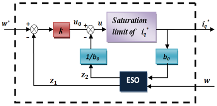
Figure 1. Block diagram of the ESO-based controller
Subsequently, we use ESO approaches to accomplish the job of developing a composite speed-loop controller. The control technique for PMSM using the ESO approach is shown in Figure 1. Take note that the provided current, shown as $i_q^*$, is subject to a constraint in this figure. When establishing a threshold for the absolute value of $i_q^*$, which is often denoted as $i_{\text {qmax }}>0$, it is important to consider saturation. The relationship between $i_q^*$ and $\mathrm{u}$ is hence
$i_q^*=\operatorname{sat}(u)= \begin{cases}u, & |u| \leq i_{qmax } \\ i_{qmax } \cdot \operatorname{sign}(u), & |u|>i_{qmax }\end{cases}$ (8)
The DOB is a widely used state observer that has an extra feature. The ESO has the ability to both rebuild the state and assess external disturbances [16].
$\dot{\omega}=\frac{K_t i_q}{J}-\frac{B \omega}{J}-\frac{T_L}{J}=a(t)+b_0 i_q^*$ (9)
The findings obtained from the surface-mounted PMSM model, which is based on the rotor coordinates (d-q axes), are as follows:
$x_1=\omega, x_2=a(t)$ (10)
The state equation shown below may be obtained by transforming the dynamics of system (9).
$\dot{x_1}=x_2+b_0 i_q^*, \dot{x}_2=c(t)$ (11)
where, $c(t)=\dot{a}(t)$. To generate a linear equivalent single output ESO for the value (11), the following approach may be used.
$\dot{z}_1=z_2-2 p\left(z_1-\omega\right)+b_0 i_q^*$ (12)
$\dot{z}_2=-p^2\left(z_1-\omega\right)$ (13)
In this scenario, p is the necessary ESO double pole, with p being greater than 0. Here, z1(t) denotes an estimation of the speed output, while z2(t) indicates an estimation of the combined disturbances a(t), specifically z1(t) and z2(t) a(t). A composite control rule for the speed loop z is then formulated.
$i_q^*=sat\left(u_0-\frac{z_2}{b_0}\right)$ (14)
$u_0=k\left(\omega^*-z_1\right)$ (15)
Speed sensorless control of electric drives, has become increasingly attractive. This control is of economic interest, improves reliability, decrease the maintenance costs and avoids the fragility and difficulty of installing the mechanical speed sensor. In addition,sensors are not reliable in explosive environment like in chemical industries. The speed must then be reconstructed by estimation. The MRAS technique is well recognised as a reliable and direct approach for sensorless estimation. The performance of the system exhibits reliability and robustness, especially under conditions including regenerative braking or frequent rapid alterations in speed. Based on the concepts of MRAS, the parameters of the adjustable model are modified by a comparison of the outputs generated by the adjustable model and the reference model. The adaptive law incorporates errors [21-23]. Through the use of the adaptive process, it becomes feasible to make estimations about both the speed and position of the rotor.
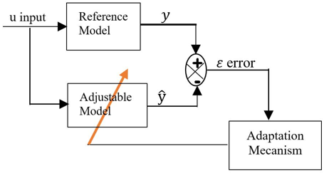
Figure 2 depicts the core constituents of MRAS, which consist of three primary elements: an adjustable model, a reference model, and an adaptation mechanism. Both the reference and modifiable models are excited by the same external input, $y$ and $\hat{y}$ are the state vector of the reference and the adjustable model. In contrast to the reference model, which is expected to be unaffected by the estimating parameter, the adjustable model should be reliant on it. The use of an estimated system to determine stator d-q axis currents and rotor speed is a result of incorporating the inaccuracies associated with these two variables into the adaptation process. The foundational ideas of a reference model and an adaptive model serve as the basis for the MRAS approach [24].
Figure 2. Speed estimation scheme for model reference adaptive system
The mathematical representation of the d-q axis currents of PMSM may be presented as a reference model.
$\left[\begin{array}{l}\dot{i}_d \\ \dot{i}_q\end{array}\right]=\left[\begin{array}{cc}-\frac{R}{L} & \omega_r \\ -\omega_r & -\frac{R}{L}\end{array}\right]\left[\begin{array}{l}i_d \\ i_q\end{array}\right]+\left[\begin{array}{c}\frac{u_d}{L} \\ \frac{u_q-\psi_{p m} \omega_r}{L}\end{array}\right]$ (16)
The mathematical model of PMSM d-q axis currents containing the parameter to be estimated as an adjustable model, according to MRAS, this model is expressed as:
$\left[\begin{array}{l}\hat{i}_d \\ \hat{\dot{i}}_q\end{array}\right]=\left[\begin{array}{cc}-\frac{R}{L} & \widehat{\omega}_r \\ -\widehat{\omega}_r & -\frac{R}{L}\end{array}\right]\left[\begin{array}{l}\hat{i}_d \\ \hat{i}_q\end{array}\right]+\left[\begin{array}{c}\frac{u_d}{L} \\ \frac{u_q-\psi_{p m} \widehat{\omega}_r}{L}\end{array}\right]$ (17)
The formulation of the adaptive mechanism for the MRAS technique will be undertaken subsequent to the advancement of the adjustable and reference models. Under ideal conditions, there is no discrepancy between the two models. Consequently, it is essential to provide a precise definition for the word "state error" as follows:
$\varepsilon_d=i_d-\hat{i}_d$ and $\varepsilon_q=i_q-\hat{i}_q$ (18)
The state error equation of Eq. (16) minus Eq. (17) is as follows:
$\left[\begin{array}{c}\dot{\varepsilon}_d \\ \dot{\varepsilon}_q\end{array}\right]=\left[\begin{array}{cc}-\frac{R}{L} & \widehat{\omega}_r \\ -\widehat{\omega}_r & -\frac{R}{L}\end{array}\right]\left[\begin{array}{l}\varepsilon_d \\ \varepsilon_q\end{array}\right]+\left[\begin{array}{c}i_q \\ -i_d-\frac{\psi_{p m}}{L}\end{array}\right]\left(\omega_r-\widehat{\omega}_r\right)$ (19)
As a result, the PMSM state error model is as follows:
$\dot{\varepsilon}=A \varepsilon+B x$ (20)
Popov stability may be used to build the adaptive law:
$\begin{gathered}\widehat{\omega}=K_i \int\left(-\varepsilon_q i_d-\varepsilon_q \frac{\psi_{p m}}{L}\right) d t +K_p\left(\varepsilon_d i_d-\varepsilon_q i_d-\varepsilon_q \frac{\psi_{p m}}{L}\right)+\widehat{\omega}_r(0)\end{gathered}$ (21)
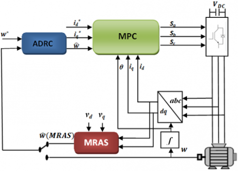
Figure 3 illustrates the global diagram of ADRC-based MPC with speed MRAS estimator.
Figure 3. Comprehensive layout of the MPC incorporating an ADRC and an MRAS speed estimator in a global context
The simulation findings used in this research work with simulation time-step 0.5 (at 0.15 second applied reference speed and at 0.3 second applied Torque load) second are based on the parameter values of the system being investigated as follows:
The characteristics of the PMSM utilized are: Stator Resistance R = 2.3 ohms, Stator inductance L = Ld = Lq = 0.0076 H, Moment of inertia J = 0.0032 Kg.m2, Friction coefficient Bm = 0.0003 Nm/rad/sec, Rotor magnet flux $\psi_{p m}$= 0.4 V/rad/sec, Rated speed N = 1500 rpm, Number of pole pairs P = 4 pairs of poles.
The solver used: Fixed step ode4 (Runge-Kutta) and Fixed step size 1e-5.
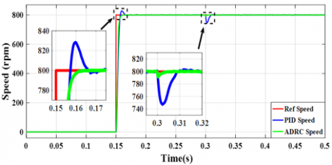
The theoretical frameworks outlined in this study have been examined, simulated, and executed to verify the efficacy of the control method and then assess the system's performance. The simulation findings used in this research work are based on the parameter values of the system being investigated, which are shown in Table A1. The verification of the system's resilience and stability has been conducted using computer simulation. The following results demonstrate the performance analysis conducted on FCS-MPC when combined with the ADRC and MRAS estimator. The first paragraph presents a comparison between the MPC technique and the PID and ADRC methods in the context of the external speed loop. The following subsection provides an account of the outcomes derived from the use of DOB and MRAS for load torque disturbance and rotor speed estimation. From the velocity simulation findings presented in Figure 4, it is discernible that the ADRC algorithm swiftly attains stability at a time instant of 0.16 seconds. In contrast, the PID control algorithm exhibits pronounced oscillatory behavior and significant overshoot. Notably, when subjected to a sudden load disturbance of 19 Newton-meters at 0.3 seconds, the PID control algorithm registers a nadir speed of 750 revolutions per minute (rpm), whereas the ADRC algorithm achieves a superior minimum speed of 794 rpm. Remarkably, the ADRC system promptly returns to a steady-state condition within a mere 0.006 seconds following the load perturbation, whereas the PID control system requires 0.013 seconds to restore its steady-state performance.
Figure 4. Speed Simulation results for the speed response of PID, and ADRC with start-up and load disturbance at operation speed of 800rpm estimation scheme for model reference adaptive
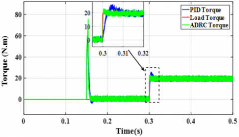
Figure 5 illustrates the outcomes of torque simulations. Notably, during the initial startup phase, it is evident that the PID control algorithm exhibits considerably greater oscillation amplitude and temporal extent compared to the ADRC. Following the abrupt introduction of a 19 N.m load at 0.3 seconds, the PI controller registers a torque amplitude of 24 N.m, whereas the ADRC demonstrates a more modest torque amplitude of 20 N.m. Moreover, it is noteworthy that the ADRC system exhibits a shorter recovery time compared to the PI controller. Furthermore, it is discernible that the torque fluctuation in the PI controller surpasses that of the ADRC system.
Figure 5. Simulation results for Electromagnetic torque with load application of 19 N.m at t=0.3
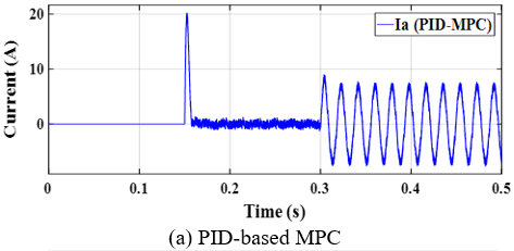
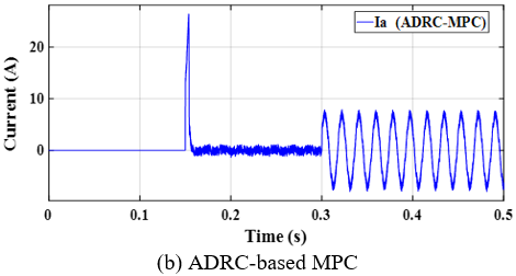
The stator phase current is shown in Figures 6 and 7, along with Total Harmonic Distortion (THD) analysis. Low ripples may be seen in Figure 6's torque response, but the ADRC-MPC in that figure lowers overshoot and responds to load more quickly.
Figure 6.Stator phase current Ia
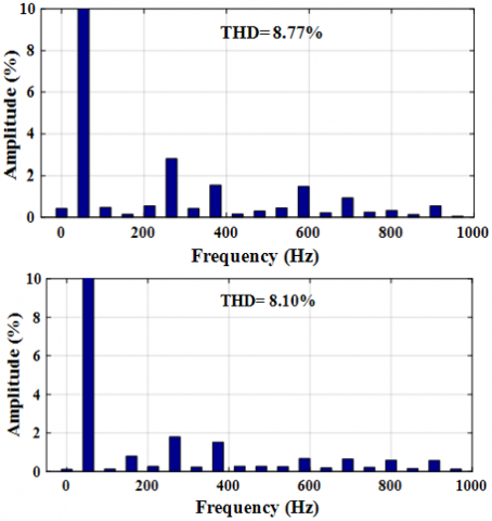
Figure 7. Spectrum of THD for stator phase current Ia
THD is a crucial metric included in these standards to systematically and objectively assess the quality of power systems. Its purpose is to enhance power system quality and minimize distortion levels. THD is a measure of the difference in energy percentage between the fundamental component and the other harmonic components in a signal. In power systems, the fundamental component is often the most significant one, particularly for current, which is important for our system. Figures 6 and 7 depict the current waveform as well as the overall harmonic distortion that it demonstrates. Both figures are shown below. In compared to the PI-MPC, which has a THD of 8.77 percent, the ADRC-based MPC has a THD that is 8.10 percent lower. The disturbance compensation capability is a property that contains adequate regulatory control property and increased robustness against unknown disturbances. It is also known as the power to compensate for disturbances. The current waveform and its overall harmonic distortion are shown in Figures 6 and 7. When compared to PI-MPC (8.77%), the ADRC-based MPC has a lower THD (8.10%), this is known as the disturbance compensation ability.
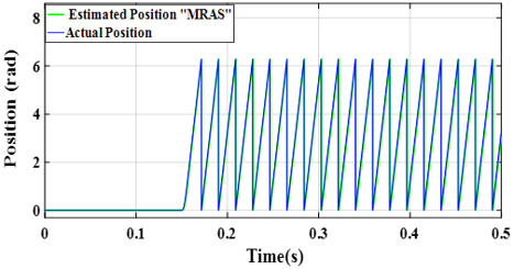
Figure 8 shows cases the rotor's corresponding estimated and actual positions, where each division corresponds to an angular measurement of 2 radians.
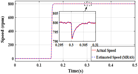
The speed simulation outcomes depicted in Figure 9 demonstrate the progression of both actual speed and MRAS-estimated speed, escalating from 0 to 800 rad/min at 0.15 seconds. Upon the imposition of a load at 0.3 seconds, it becomes evident that ADRC-MPC yields a notably brief tracking duration and transition time to attain the targeted speed. Furthermore, there is a close alignment between the estimated speed and the actual speed, indicating a nearly impeccable concordance.
Figure 8. Waveforms of estimated position and actual position
Figure 9. Waveforms of estimated speed and actual speed
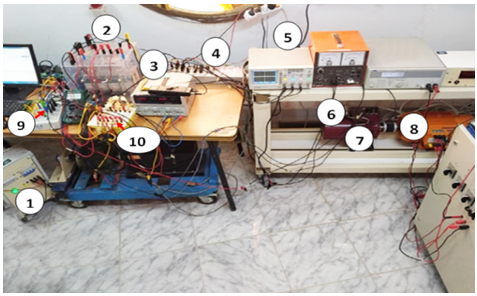
The Figure 10 presents the experimental bench of PMSM drive system.
The PMSM motor The motor utilized is three-phase. with the power of 3 kW. The Table A1 included to the Appendix contains the remaining parameters. For a guide, the simulations utilize the same motor. To illustrate the approach's superiority and efficacy, it was compared to PID-MPC, and the results were obtained under a variety of scenarios, beginning with no load , subsequently supplying a load torque and varying the reference speed, and then removal of the load torque. Figure 11 shows all of the obtained outcomes, which were then sorted as follow the PID-MPC in the top and ADRC-MPC in the Bottom, respectively under start-up and load disturbance conditions.
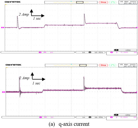
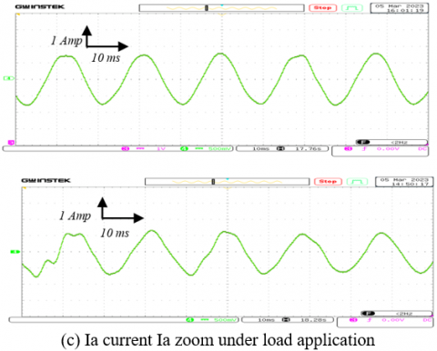
Figure 12 illustrates the results that have been obtained from the same preceding scenario. This figure presents the iq current and phase current Ia. It is organized as follows: PID-MPC in the top and ADRC-MPC in the bottom.
Figure 10. Experimental bench of PMSM drive system
The components of the experimental bench of the platform are given in Figure 10. It is essentially composed of the following components:
1-Autotransformer (0-450 V)
2-Inverter (Semikron power converter with nominal characteristics: 1000 V, 30 A)
3-Power Supply (0 V, 30 V, 0 A, 3 A)
4-dSpace 1104 acquisition card connected to the computer.
5-Oscilloscope
6-Incremental encoder
7-PMSM (3 kW)
8-Load
9-Current mesurment
10-Amplifier(5v-15v)
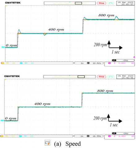
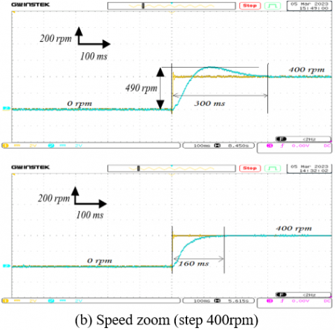
The comparative analysis of the speed performance of PID-MPC and ADRC-MPC is illustrated in Figure 11(a), specifically highlighting their responsiveness across various speed step changes, from startup to load application.
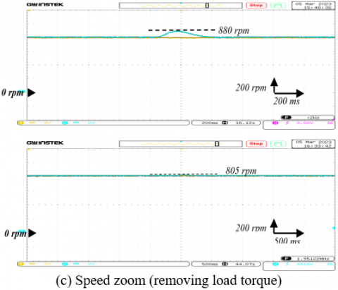
It is evident from the graphical representation that, under all operational scenarios, the dynamic response exhibited by the ADRC-MPC approach surpasses that of the PID-MPC method, as clearly depicted in Figures 11(b) and (c), which show the speed variation and load removal cases, respectively. We can see that there is no obvious overshoot in the case of ADRC-MPC with time response of only 160 ms, as opposed to PID-MPC, which exceeds the reference speed by 90 rpm (490 rpm) with time response of 300 ms,. Also, when we apply the load torque, we see that the speed declines till it hits 380 rpm, which is 20 rpm slower than the reference speed. At the same time, we don't see much of a difference in speed while using ADRC -MPC.In ADRC-MPC, when the load torque is removed at the instant 8.5 seconds, the speed is quickly restored to the reference, The speed measurement barely exceeded the reference speed by 5 rpm, however in the case of PID, we see an 80 rpm (880 rpm) exceedance. These latest findings illustrate the superior robustness of ADRC-MPC over PID-MPC.
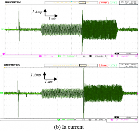
Figure 12 demonstrates the phase current Ia of the PID-MPC and ADRC-MPC, as well as a zoom of the current Ia. The current Ia in Figure 12(c) is sinusoidal, and there is nearly no difference between PID-MPC and ADRC-MPC, proving the efficiency of the suggested approach.
Figure 11. Experimental results for the speed response of PID, ADRC, respectively under start-up and load disturbance conditions
Figure 12. Experimental results for q-axis current and the phase current Ia of PID, ADRC, respectively under start-up and load disturbance conditions
This can also be seen in the zoom-in on Figure 12(b), which is a case of applying the load torque. We observe that the results are very similar between the two techniques, as the form of the current iq is almost identical while the phase current is sufficiently sinusoidal, making PID compensation with ADRC a very good solution considering the advantage it provides in terms of response time and robustness.
In this article, we have accomplished and presented a combination of two modern control technologies, namely MPC and ADRC. The first method has proven its effectiveness in terms of performance, speed of response, and simplicity of principle. As for ADRC, it is a modern technology that we have applied as a speed regulator instead of classic and well-known regulators such as the PID and Fuzzy Logic Regulator (FL). The study was carried out using simulations with Simulink as well as experimental work and comparing it with PID integrated with MPC under different conditions, first with no load, then with applying a load Torque of 19 Nm, and under different speeds (400 rpm and 800 rpm). The results showed that the ADRC technology with MPC outperformed PID-MPC in terms of time response (160 ms for ADRC-MPC rather than 300 ms in PID-MPC), overshoot, and robustness, especially dealing with the change in torque load as shown in the experimental result above. The current form also clearly shows in the simulation result that THD=8.10 in ADRC-MPC and THD=8.77 in PID-MPC. The work has been done by integrating MRAS to eliminate the speed sensor, and it shows good efficiency, which adds to decreasing the system's price and size while enhancing its efficiency.
Table A1. Parameters of the three-phase PMSM used in the simulation in and experimental (SI units)
|
Parameters |
Values |
|
Stator Resistance R |
2.3 ohms |
|
Stator inductance L = Ld = Lq |
0.0076 H |
|
Moment of inertia J |
0.0032 Kg.m2 |
|
Friction coefficient Bm |
0.0003 Nm/rad/sec |
|
Rotor magnet flux $\psi_{p m}$ |
0.4 V/rad/sec |
|
Rated speed N |
1500 rpm |
|
Number of pole pairs P |
4 pairs of pole |
[1] Huang, Y., Huang, W., Chen, S., Liu, Z. (2019). Complementary sliding mode control with adaptive switching gain for PMSM. Transactions of the Institute of Measurement and Control, 41(11): 3199-3205. https://doi.org/10.1177/0142331219826664
[2] Qi, L., Bao, S., Shi, H. (2015). Permanent-magnet synchronous motor velocity control based on second-order integral sliding mode control algorithm. Transactions of the Institute of Measurement and Control, 37(7): 875-882. https://doi.org/10.1177/0142331213495886
[3] Melfi, M.J., Evon, S., McElveen, R. (2009). Induction versus permanent magnet motors. IEEE Industry Applications Magazine, 15(6): 28-35. https://doi.org/10.1109/MIAS.2009.934443
[4] Zhang, Y., Xu, D., Liu, J., Gao, S., Xu, W. (2017). Performance improvement of model-predictive current control of permanent magnet synchronous motor drives. IEEE Transactions on Industry Applications, 53(4): 3683-3695. https://doi.org/10.1109/TIA.2017.2690998
[5] Casadei, D., Profumo, F., Serra, G., Tani, A. (2002). FOC and DTC: Two viable schemes for induction motors torque control. IEEE Transactions on Power Electronics, 17(5): 779-787. https://doi.org/10.1109/TPEL.2002.802183
[6] Zhang, Y., Zhu, J. (2010). Direct torque control of permanent magnet synchronous motor with reduced torque ripple and commutation frequency. IEEE Transactions on Power Electronics, 26(1): 235-248. https://doi.org/10.1109/TPEL.2010.2059047
[7] Jung, J.W., Leu, V.Q., Do, T. D., Kim, E.K., Choi, H.H. (2014). Adaptive PID speed control design for permanent magnet synchronous motor drives. IEEE Transactions on Power Electronics, 30(2): 900-908. https://doi.org/10.1109/TPEL.2014.2311462
[8] Ammar, A., Talbi, B., Ameid, T., Azzoug, Y., Kerrache, A. (2019). Predictive direct torque control with reduced ripples for induction motor drive based on T-S fuzzy speed controller. Asian Journal of Control, 21(4): 2155-2166. https://doi.org/10.1002/asjc.2148
[9] Yeoh, S.S., Yang, T., Tarisciotti, L., Hill, C.I., Bozhko, S., Zanchetta, P. (2017). Permanent-magnet machine-based starter-generator system with modulated model predictive control. IEEE transactions on transportation electrification, 3(4): 878-890. https://doi.org/10.1109/TTE.2017.2731626
[10] Moon, H.T., Kim, H.S., Youn, M.J. (2003). A discrete-time predictive current control for PMSM. IEEE Transactions on Power Electronics, 18(1): 464-472. https://doi.org/10.1109/TPEL.2002.807131
[11] Huang, Y., Xue, W. (2014). Active disturbance rejection control: Methodology and theoretical analysis. ISA Transactions, 53(4): 963-976. https://doi.org/10.1016/j.isatra.2014.03.003
[12] Ding, X., Guo, H., Du, M., Li, B., Liu, G., Zhao, L. (2014). Effect of saturation on iron loss in PMSM. In 2014 17th International Conference on Electrical Machines and Systems, Hangzhou, China, pp. 3356-3360. https://doi.org/10.1109/ICEMS.2014.7014071
[13] Yang, G., Zhang, S., Zhang, C. (2020). Analysis of core loss of permanent magnet synchronous machine for vehicle applications under different operating conditions. Applied Sciences, 10(20): 7232. https://doi.org/10.3390/app10207232
[14] Ogab, C., Hassaine, S., Sbaa, M., Haddouche, K., Bendiabdellah, A. (2021). Sensorless digital control of a permanent magnet synchronous motor. Journal Européen des Systèmes Automatisés, 54(3): 511-517. https://doi.org/10.18280/jesa.540315
[15] Wang, B., Jiao, J., Xue, Z. (2023). Implementation of Continuous control set model predictive control method for PMSM on FPGA. IEEE Access, 11: 12414-12425. https://doi.org/10.1109/ACCESS.2023.3241243
[16] Kakouche, K., Oubelaid, A., Mezani, S., Rekioua, D., Rekioua, T. (2023). Different control techniques of permanent magnet synchronous motor with fuzzy logic for electric vehicles: Analysis, modelling, and comparison. Energies, 16(7): 3116. https://doi.org/10.3390/en16073116
[17] Ahmed, A.A. (2015). Fast-speed drives for permanent magnet synchronous motor based on model predictive control. In 2015 IEEE Vehicle Power and Propulsion Conference, Montreal, QC, Canada, pp. 1-6. https://doi.org/10.1109/VPPC.2015.7352946
[18] Hou, Q., Ding, S. (2021). Finite-time extended state observer-based super-twisting sliding mode controller for PMSM drives with inertia identification. IEEE Transactions on Transportation Electrification, 8(2): 1918-1929. http://doi.org/10.1109/TTE.2021.3123646
[19] Tian, M., Wang, B., Yu, Y., Dong, Q., Xu, D. (2021). Discrete-time repetitive control-based ADRC for current loop disturbances suppression of PMSM drives. IEEE Transactions on Industrial Informatics, 18(5): 3138-3149. http://doi.org/10.1109/TII.2021.3107635
[20] Guo, B.Z., Zhao, Z. L. (2011). Extended state observer for nonlinear systems with uncertainty. IFAC Proceedings Volumes, 44(1): 1855-1860. https://doi.org/10.3182/20110828-6-IT1002.00399
[21] Shweta, B., Sadhana, V. (2022). Model predictive control and higher order sliding mode control for optimized and robust control of PMSM. IFAC-Papers Online, 55(22): 195-200. https://doi.org/10.1016/j.ifacol.2023.03.033
[22] Badini, S.S., Khan, Y.A., Verma, V. (2022). K-MRAS based mechanical sensorless vector controlled PMSM drive. In 2022 2nd International Conference on Emerging Frontiers in Electrical and Electronic Technologies, Patna, India, pp. 1-6. https://doi.org/10.1109/ICEFEET51821.2022.9847763
[23] Kumar, S., Singh, B., Sreejith, R. (2021). MRAS based sensorless PMSM drive with regenerative braking for solar pv-battery powered EV. In 2020 3rd International Conference on Energy, Power and Environment: Towards Clean Energy Technologies, Meghalaya, India, pp. 1-6. https://doi.org/10.1109/ICEPE50861.2021.9404416
[24] Badini, S.S., Verma, V. (2019). A novel MRAS based speed sensorless vector controlled PMSM drive. In 2019 54th International Universities Power Engineering Conference, Bucharest, Romania, pp. 1-6. https://doi.org/10.1109/UPEC.2019.8893607