Lightweight RNN-Based Model for Adaptive Time Series Forecasting with Concept Drift Detection in Smart Homes

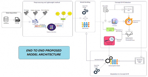
As shown in Figure 2, the proposed methodology is an end-to-end process consisting of several stages. It starts with the collection of time series data and then proceeds to a lightweight pre-processing phase that includes the essential step of feature selection. The subsequent phase involves building the RNN model, with careful attention given to training and hyperparameter tuning using HyperOpt. After generating forecasts using unseen data, a concept drift detection mechanism is introduced, which involves monitoring performance through a sliding error window of recent data. Once concept drift is detected by the model, the model adaptation phase is initiated, and the model is retrained on a retraining window of recent data to adapt to new data patterns if the pattern was not already seen by past tracked models. In the following sections, each phase is discussed in greater detail.

Figure 2. End to end model architecture

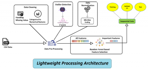
4.1 Lightweight method

Time series data typically has a high volume; hence, model training and retraining can take a lot of time. Thus, making a model lightweight is beneficial. Existing techniques to make a model lightweight include down-sampling, feature selection, segmentation, and stratification. All these techniques have their own advantages and drawbacks. However, out of them, feature selection is what we found to be most impactful on the quality of forecasting. Feature selection is a technique to choose only those features from the data that have a high influence on the target feature. In other words, it discards redundant and useless features from the data before it is fed to the model. This allows the model to learn from the selected quality data and thus potentially improve the forecasting quality.

3.png

Figure 3. Lightweight model architecture

As shown in Figure 3, for the proposed model, we used a random forest-based feature selection technique to make the model lightweight.

4.1.1 Random forest based feature selection

Random forest-based feature selection is a popular technique used to select relevant features from data. The method works by constructing multiple decision trees based on a randomly selected subset of data and features. The algorithm assigns an importance score to each feature based on how well the feature separates the target variable. Features with higher importance are deemed more valuable. This process is carried out multiple times, and the average importance of each feature across the entire random forest is calculated and used to finally decide which features are going to be selected. By default, the algorithm selects those features with a higher feature importance than the average feature importance across all the features. The final selected features are fed to the forecasting model as input.

The computation of importance is measured by the metric Mean Squared Error (MSE), MSE is calculated as follows,

$M S E=\frac{1}{N} \sum_{i=1}^N\left(y_i-\mu\right)^2$            (1)

where, y is the value of target, N is the number of instances and u is the mean value of the target over all the data instances.

For all the nodes of the trees in the Random Forest the MSE is calculated. Then the importance of each of the nodes is computed as follows.

${Imp}_j=W_j C_j-W_{l j} C_{l j}-W_{r j} C_{r j}$                           (2)

where, Imp, stands for the importance of node j. W stands for weighted number of samples reaching node j. C is the MSE at node j, j and rj subscripts stand for left and right child after the split at node j respectively.

The importance of each individual feature is then calculated as follows.

$F I_i=\frac{\sum_{j:  { node } j { splits on feature } i} {Imp}_j}{\sum_{k \in  { all nodes }} {Imp}_k}$             (3)

where, FI_i stands for feature importance of i^th feature and Imp_j is the importance of node_j. The feature importance is normalized in the range of 0 to 1. The feature importance is normalized in the range of 0 to 1 by dividing the feature importance values by the sum of all feature importance.

NormFI $_i=\frac{F I_i}{\sum_{j \in  { all features }} F I_j}$               (4)

The average feature importance of each feature across all the trees in the Random forest is the final feature importance of the features,

$R F_{-} F I_i=\frac{\sum_{j \in  { all trees }}  { NormFI } j_j}{T}$                   (5)

where, RF_FI_i is the feature importance of feature i for the entire random forest, NormFI_j is the normalized feature importance at the j^th tree and T is the total number of decision trees in the forest.

By utilizing this feature selection process, the forecasting model gets only relevant and important features as input and not unwanted, noisy features, this helps improve the quality of the forecast and makes the model lightweight in nature.

4.2 Recurrent neural networks as base model

The base model algorithm is RNN. As shown in Figure 4, Recurrent neural networks are a kind of neural network that are capable of handling sequential data where the input data is a sequence of vectors.

4.png

Figure 4. RNN algorithm flow

It can be text, speech, or time-series data. Unlike traditional neural networks that process each input piece of data independently, RNNs maintain an internal memory state that allows them to process sequences of arbitrary length. In simple words, RNNs can predict future values based on both current and past values, i.e., they have memory.

The RNN architecture consists of input X, hidden state h, and output Y. There are weights associated with each of them, namely, input weights Wx, recurrent or hidden layer weights Wh, and Output weights Wy, whereas bh and by are the biases corresponding to the hidden layer and output layer, respectively. At each time step 1, RNN takes the input vector Xt and the hidden state h(t-1) of the previous time step. The network then computes a new hidden state representation ht as a function of the current input and previous hidden state and generates an output Yt based on the new hidden state. Overall, RNNs and their more advanced versions like Long-Short-Term Memory (LSTM) and Gated Recurrent Unit (GRU) are powerful tools for time series forecasting and have been used successfully in a wide range of applications.

Mathematically, at each timestep, the computation of hidden state h and output Y is based on formulas as follows:

h_t=ƒ(W_x*X_t+W_h*h_t-1+b_n)              (6)

Y₁=f(Wy*h_t+b_y)                    (7)

where, ƒ denotes the activation function, which is used to apply non-linear transformations to the data, which helps with training the neural networks. We used the TensorFlow Keras framework to build the RNN model in our study. RNN, like any neural network model, has a lot of hyperparameters to be set before training it. The complete information on the different hyperparameters of a RNN is provided in Table 1 as follows:

Table 1. Hyper-parameters of RNN

We train the model on a set of training data, and then to tune the hyperparameter, we use the Bayesian optimization algorithm. Bayesian optimization is a machine learning technique for tuning the hyperparameters of a given model. The idea behind it is to iteratively build a probability model of the objective function (RMSE of validation data). It then makes intelligent choices about where to sample the hyperparameter space next. Within predetermined parameters, the hyperparameter search space was defined. During optimisation, 50 trials were carried out in order to iteratively improve the performance of the model. By using the probability estimates of the model, Bayesian optimization can balance the exploration of new regions of the search space with the exploitation of promising regions that have already been sampled.

HyperOpt is a Python library that provides an implementation of Bayesian optimization for hyperparameter tuning. To use HyperOpt for hyperparameter tuning, the user defines a search space of possible hyperparameter values and an objective function (such as validation RMSE). HyperOpt then samples from the given search space, evaluates the objective function, and updates the probabilistic model. This process continues for a given number of trials.

Finally, after hyperparameter tuning, we get the final trained model with the best possible hyperparameters, ready to predict on the unseen data.

4.3 Concept drift detection

To address the issue of concept drift, As shown in Figure 5, the proposed model monitors its performance over a window of recent data. The window is called Error Window W and holds the latest w data points from the data stream. The model's performance (Accuracy for classification and RMSE or other regression metrics) is measured against the error window W. A defined error threshold is set beforehand based on the model's performance on the training data itself, and when the model's performance crosses the threshold, concept drift is detected, indicating a significant change in the data pattern. Once drift is detected, the model needs to be updated to adapt to the new data pattern and improve its performance. Because of its susceptibility to changes in prediction errors, RMSE was selected as the method for detecting concept drift. When used, it guarantees efficient model performance monitoring, identifying patterns in data deviations and triggering timely adjustments for increased predicting accuracy. So, assuming RMSE as the error metric, the concept drift detection algorithm is as follows:

Concept Drift Detection (ground_truth, pred, W, Th):

ground truth: Actual values

pred: predicted values

W: error window of size w

Th: Performance threshold

START

Running_error: RMSE over the latest window W, $\sqrt{\frac{1}{w} \sum_{i=1}^w\left(\text { pred }_i-\text { ground_ruth }_i\right)^2}$; If (Running_error > Th):

Concept drift is detected;

Else:

Get Next model prediction;

Get next ground_truth from data stream;

Update the error window W;

Check for concept drift again;

END

5.png

Figure 5. Concept drift detection method architecture

In this section, we present a detailed analysis of the performance metrics and provide insights into the strengths of the proposed model. We start by describing the experimental setup and the evaluation criteria used in this study Next, we showcase the time and memory consumption analysis of the proposed model, followed by discussion on concept drift detection and adaptation to the drift. We show how feature selection is important for achieving better results. We also compare the performance of the proposed model with a recent research work DSTP-RNN [9] on the SML2010 dataset to show that the proposed model outperforms it comprehensively.

6.1 Pre-processing and feature selection of data

Pre-processing is a necessary step to prepare the data in a way that can be fed to the model training phase. At first, we combined the data and time columns and set them as indexes for visualization purposes Since the SML 2010 dataset did not have missing values and all the features were numerical, additional steps to impute missing values or categorical feature encoding were not required.

We applied the random forest-based feature selection technique to the prepared data with a 70:30 split, 100 estimators, and a random seed of 0 for reproducibility, and the results were provided in Table 4.

Table 4. Results of random forest based feature selection

We checked for outlier in the dataset using Z score criteria (23) but the data does not contain any outliers.

6.2 Train-test split

To compare the results of the proposed model with those of the DSTP-RNN model, we set the train-test split the same as in that paper. The first 2000 instances are selected as the training set, and the last 763 data instances are selected as a holdout test set. During the training, 10% of the training set is used as a validation set for tuning the hyperparameters of the model. The RMSE is chosen as the evaluation metric for the experiments. For the purpose of evaluating the model, the choice to divide the data into training and test sets is essential. It makes evaluating the model's ability to generalise to new data possible. However, the robustness of the model may be limited by the use of just 763 data points for testing. Its performance in a variety of contexts would be better validated with a broader test set, reducing the possibility of overfitting to the particular holdout data.

6.3 Model specifications

A Recurrent Neural Network is used as the base model due to its effectiveness in time series forecasting and ability to find complex data patterns. The HyperOpt library is used for tuning the hyperparameters using the Bayesian Optimization technique. The final RNN model used for the SML 2010 dataset has one hidden layer with 12 units. The lag sequence parameter was chosen to be 12. An Adam optimizer with a learning rate of 0.001 is used for the training. The activation functions for the hidden and output layers are tanh and linear, respectively. A batch size of 256 is selected with 1500 epochs. L1 regularization of the value 0.0001 is used in the hidden layer to counter any possible overfitting. The model is trained to forecast the next 30 future values of the time series at every step.

6.4 Memory and time consumption analysis

To show the lightweight nature of the proposed model, we measured the time and memory consumption of the model in the training phase with and without the feature selection step. The results show that the feature selection step essentially helps the model run faster and requires less runtime memory. All the experiments were conducted on a machine with an 11th Gen Intel (R) Core (TM) i5-processor with a clock speed of 2.60 GHz, 16 GB of RAM, and 4 Core(s). The results are provided in Table 5 and Table 6.

Table 5. Memory consumption by the dataset with and without feature selection

Table 6. Time consumption for training by the dataset with and without feature selection

From the above results, we can see that the same RNN model takes more time and memory when all the features of the dataset are used compared to when only the important features selected by the Random Forest based feature selection algorithm are used. We see a huge 86.7% reduction in memory consumption, which can save a lot of memory as the time series data tends to have a high volume. Also, the reduction in time consumption is 16.2%, which, by intuition, we can say will increase significantly when the volume of the data increases.

6.5 Model performance with and without feature selection analysis

To show that feature selection helps the model learn from important relevant features and not get confused with redundant noisy features, we compared the results of the proposed model with and without feature selection with identical settings of hyperparameters. The result is provided in Table 7.

Table 7. Model performance on test dataset with and without Feature Selection

Hence, we get about an 83.8% improvement in RMSE. The reason behind that could be that the features that were dropped using the Random forest-based feature selection algorithm were noisy and did not contribute much new information to modelling the target feature. Hence, dropping those features helps the model perform better.

6.6 Concept drift detection and adaptation analysis

As discussed, the proposed model detects concept drift by monitoring the model's performance over the defined error window. Whenever the model performance RMSE goes above a set threshold, concept drift is detected. The threshold is set based on the model performance on the training set itself, i.e., the training RMSE as provided in Table 8.

Table 8. Training RMSE on the dataset

To have some flexibility in the drift detection, we set the RMSE threshold at 120% of the training RMSE as provided in Table 9.

Table 9. Performance threshold for the dataset

The error window size is chosen as follows based on intuition and trials as shown in Table 10.

Table 10. Error window size for the dataset

Because the SML 2010 dataset does not have any concept drift, we injected artificial drift into the test data to see how the proposed model detects it. We injected incremental drift of a magnitude of half the mean of the target from the 200th instance onwards. The test data before and after drift injection is as follows:

As the model detects concept drift, the immediate next action should be to retrain the model so that it can adapt to the new concepts in the data stream. We define a retraining window R that holds the most recent R data points from the data stream. The retraining uses only the data within window R. During the retraining to tune some of the hyper-parameters, we employed HyperOpt again. We split the retraining window 70:30 and use the last 30% as validation data for the tuning. Once tuning is done and the best-performing hyperparameters are found, we finally retrain the model for the entire retraining window using the best set of hyperparameters. To avoid too frequent retraining, we specify a minimum gap between two retraining equal to the size of the error window. Also after every drift detection we check if any of the past 10 saved models produce performance metric better than the threshold set. If yes, the best performing past model replaces the current model and there is no need for retraining for that particular concept drift detection instance. The retraining window size is selected as follows and is provided in Table 11.

The selection of 256 batches and 1500 epochs was determined by computational performance as well as empirical findings. Through experimentation, these parameters were found, striking a balance between computational resources and model convergence. The model's performance and resource usage on the specified hardware are optimized while effective training is ensured by the chosen settings. Next, to see how retraining helps with concept drift adaptation. We measured the model performance in terms of RMSE, with and without retraining on the drift injected test data of the SML 2010 dataset and the comparison is provided in Table 12.

Table 11. Retraining window size for the datasets

Table 12. Performance measure RMSE of the proposed model before and after drift addition, with and without drift detection and retraining