Farid Oudjama*![]() | Abdelmadjid Boumediene
| Abdelmadjid Boumediene![]() | Khayreddine Saidi
| Khayreddine Saidi![]() | Mohammed Messirdi
| Mohammed Messirdi![]()
© 2023 IIETA. This article is published by IIETA and is licensed under the CC BY 4.0 license (http://creativecommons.org/licenses/by/4.0/).
OPEN ACCESS
Permanent magnet synchronous motor-powered electric vehicles control is the subject of various research work. However, their global dynamic models are nonlinear and coupled. Therefore, to achieve efficient operation, an effective control system is crucial. In this study, we propose and compare linear H-Infinity and Galerkin approximation approach for Nonlinear H-Infinity control strategies to improve the durability and performance of post-driven speed in electric vehicles. In the case of linear systems, the linear H-Infinity controller is found by solving the algebraic equation known as the Riccati equation. On the other hand, the control problem based nonlinear H-Infinity poses challenges because it involves solving a nonlinear partial differential equation known as name of the Hamilton-Jacobi-Isaacs equation, which is difficult or even impossible to solve by using analytical methods. In these situations, the Galerkin approximation approach provides an approximation to the Hamilton-Jacobi equation solution. In order to evaluate the performance of Galerkin approximation approach and linear H-Infinity controllers, electric vehicle feedback simulations will be conducted, taking into account different constraints. The goal is to ensure efficient operation in different situations. The results demonstrate that the Galerkin approximation Approach for nonlinear H-Infinity controller reveals a similar performance and durability as the H-Infinity controller, and stands out for its ability to optimize the control system performance of the EV, providing a faster response, reducing undesirable ripples, and enhancing overall stability and precision. Generally, this comparative study brings to light the effectiveness of linear and Galerkin approximations for H-Infinity control in permanent magnet synchronous motor-powered electric vehicles. The results contribute to the advancement of control strategies and provide valuable information for the conception and employment of efficient electric vehicle control systems.
electric vehicle, permanent magnet synchronous motor, linear H-Infinity control, Algebraic Riccati equation, nonlinear H-Infinity control, Hamilton-Jacobi-Isaacs equation, the Galerkin approximation approach
An electric vehicle (EV) is, by definition, any vehicle that is propelled by an engine that runs entirely on electrical energy [1, 2]. All participants in the advanced automotive sector view electric vehicles as one of the greenest and most environmentally friendly forms of transportation. Given that the road transportation sector contributes more to atmospheric pollution than manufacturing does, it could potentially be a solution to this grave pollution scenario. However, electric vehicles are still in the experimental stage and are being modified or improved, despite substantial research on powertrains and batteries [1, 2].
Researchers can now create driver assistance systems that automate specific tasks by adding new safety devices that increase the stability of electric vehicles, where systems must act on the electric vehicle's controllability so that it reacts more quickly to user requests to drive, thanks to advancements in automation, computing, telecommunications, and tool miniaturization.
Unfortunately, despite advances in modern control theory and methods, there is no universally optimal solution for controlling electric vehicles. The complexity of the problem and the varying requirements of different applications make it difficult to determine a best control strategy. Various factors such as vehicle dynamics, drivetrain characteristics, operating conditions and control objectives contribute to complicating matters. Therefore, trade-offs between different control methods are often necessary to achieve the desired performance and meet specific requirements.
In order to obtain excellent dynamic performance, many researchers have researched the design of electric vehicles powered by permanent magnet synchronous motors (PMSM) during the past several years. The literature is currently available and covers a wide range of control schemes. These include classical control laws [2, 3], more advanced algorithms such as nonlinear control [4, 5], fuzzy logic control [6-9], sliding mode control [10-13], backstepping control [14-16], and H∞ control [17, 18]. Each of these strategies offers its own benefits and has been explored in various studies to optimize the performance of electric vehicles.
Unfortunately, despite advances in modern control theory and methods, there is no universally optimal solution for controlling electric vehicles. The complexity of the problem and the varying requirements of different applications make it difficult to determine a best control strategy. Various factors such as vehicle dynamics, drivetrain characteristics, operating conditions and control objectives contribute to complicating matters. Therefore, trade-offs between different control methods are often necessary to achieve the desired performance and meet specific requirements. Researchers continue to explore and develop new control techniques to further improve the control of electric vehicles.
The problem treated in this article aim to find a globally optimal control solution for an EV powered by a PMSM, taking into account the complexity of vehicle dynamics, transmission characteristics, operating conditions, and diverse control objectives. It provides a fresh perspective by comparing linear and Galerkin approximation approaches for nonlinear H-Infinity controllers, offering valuable insights for the development of more effective control methods in the field.
It is well known that the solution to the algebraic Riccati equation determines how to solve the linear H-Infinity control problem [19-23]. It is necessary to solve the Hamilton-Jacobi-Bellman equation for the nonlinear H-Infinity controller [24, 25]. However, finding a trustworthy and precise approximation to the solution of this partial differential equation is a challenging task, nevertheless. One such approximation technique is the Galerkin approximation. The generalized Hamilton-Jacobi-Bellman equation is derived by first reducing the Hamilton-Jacobi-Bellman equation to an infinite sequence of linear partial differential equations in order to obtain the approximation. The second stage is to utilize Galerkin's method to approximate the solutions of these linear equations. When both of these steps are combined, a control algorithm is created that converges to the best solution when the order of the approximation and the number of iterations approaches infinity [26-28].
Once the introductory part is completed, this work is structured as follows. Section 2 presents the electric vehicle that is the subject of the study, and then a state-space representation modeling follows. Section 3 discusses linear and nonlinear H-Infinity control design and Galerkin approximation approaches. The design strategy is examined in Section 4 along with its application to electric vehicles. To evaluate the effectiveness of the controller developed in this paper, an implementation and numerical simulation of the designed controller are illustrated in Section 5. The conclusions of this study are presented in Section 6.
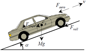
According to Figure 1, an EV system dynamics primarily consists of two components: vehicle dynamics and motor system dynamics. A transmission unit, which also contains the transmission system, connects the engine system to the electric vehicle system. In a real electric vehicle, the driver sends command signals as an acceleration or deceleration via his accelerator/brake pedals to the drive system controller. A PMSM motor is used for propulsion of the considered electric vehicle system, and a gear unit with a gear system inside of it connects a PMSM motor system to the EV system. Therefore, one can control the PMSM motor's speed to control the actual EV system.
2.1 Modeling of vehicle dynamics
Gravitational, wind, rolling resistance, and inertial forces are some of the forces that the vehicle's electric engine must overcome. Figures 1 and 2 respectively illustrate the electric vehicle configuration and a representation of the forces acting on the vehicle, where these forces can also be seen.
Figure 1. The EV's configuration
Figure 2. Forces exerted on a vehicle
The sum of all forces that act is the total resulting force and results from [29-33]:
$F=F_{\text {gravity }}+F_{\text {aerod }}+F_{\text {rolling }}+M \frac{d V_{E V}}{d t}$ (1)
Given that $F_{\text {gravity }}$ is the comprises gravitational force, $F_{\text {aerod }}$ is the aerodynamic resistance force, $F_{\text {rolling }}$ is the rolling resistance force, $M$ is the product of mass and the derivative of the linear speed is $\frac{d V_{E V}}{d t}$.
where:
The expression of the gravitational force is given by:
$F_{\text {gravity }}=M g \sin (\alpha)$ (2)
As a function of vehicle speed $V_{E V}$, the aerodynamic resistance force is expressed as:
$F_{\text {aerod }}=\frac{1}{2} \rho A_f C_D V_{E V}{ }^2$ (3)
The primary cause of the rolling resistance force is the friction between the tires of the vehicle and the road, which can be represented as:
$F_{\text {rolling }}=M g f_r \cos (\alpha)$ (4)
The resulting force $F_{\text {resulting }}$ causes the drive motor's counter torque. The following relation governs the torque:
$T_L=F_{\text {resulting }} \times \frac{r_{\text {tire }}}{G_{\text {qear }}}$ (5)
where, the EV tire radius is noted by $r_{\text {tire }}, T_L$ represent the torque that the driving motor produces, and finally $G_{\text {gear }}$ is the gear ratio.
2.2 PMSM model
For drives, induction motors, permanent magnet synchronous motors, and switching reluctance motors are frequently used. For the "best" choice, compromises between price, mass, volume, reliability, efficiency, maintenance, and other factors must be considered, much like with many other components. However, the high power density and great efficiency of PMSM make it the preferred option. The rotor d-q reference defines a permanent magnet synchronous motor, and the following equations can describe it [34, 35]:
$\left\{\begin{array}{l}\frac{d i_d}{d t}=-\frac{R}{L} i_d+P \Omega_m i_q+\frac{1}{L} u_d \\ \frac{d i_q}{d t}=-\frac{R}{L} i_q-P \Omega_m i_d-\frac{P \Phi}{L} \Omega_m+\frac{1}{L} u_q \\ \frac{d \Omega_m}{d t}=\frac{3 P \Phi}{2 J} i_q-\frac{B}{J} \Omega_m+\frac{T_L}{J}\end{array}\right.$ (6)
Within Eq. (6), $u_d, u_q$ and $i_d, i_q$ are respectively the stator voltages and currents in the $\mathrm{d}$-q reference frame; $L$ is the inductance in the d-q reference frame, $R$ represent the stator resistance, $P$ is the pole pairs, $\Phi$ is the permanent magnet flux, $J$ the motor inertia moment, $B$ is the coefficient of viscous friction and $T_L$ is the load torque.
2.3 The EV's overall dynamic model
The below equations yield the linear speed $V_{E V}$ and traction power:
$V_{E V}=\frac{r_{\text {tire }}}{G_{\text {gear }}} \Omega_m$ (7)
$P_f=V_{E V} F_R$ (8)
So combing the vehicle dynamic model, the linear speed $V_{E V}$ and the model of PMSM, The entire EV system's dynamics can be expressed as:
$\left\{\begin{array}{c}\dot{x}_1=-\frac{R}{L} x_1+\frac{P G_{\text {gear }}}{r_{\text {tire }}} x_2 x_3+\frac{1}{L} u_d \\ \dot{x}_2=-\frac{R}{L} x_2-\frac{P G_{\text {gear }}}{r_{\text {tire }}} x_1 x_3-\frac{P \Phi G_{\text {gear }}}{L r_{\text {tire }}} x_3+\frac{1}{L} u_q \\ \dot{x}_3=\frac{1}{J_{E V}}\left[\frac{3 P \Phi G_{\text {gear }}}{2} x_2-\frac{B G_{\text {gear }}}{r_{\text {tire }}} x_3-\frac{r_{\text {tire }}}{G}\left(\begin{array}{c}M g \sin (\alpha)+M g f_r \cos (\alpha)+ \\ \frac{r_{\text {tire }}{ }^2}{2 G_{\text {gear }}{ }^2} \rho A_f C_D x_3{ }^2\end{array}\right)\right]\end{array}\right.$ (9)
With: $J_{E V}=\frac{G_{g_{\text {gear }}}{ }^2+M r_{\text {tire }}{ }^2}{r_{\text {tire }} G_{\text {gear }}}$ which represent the total inertia of the electric vehicle, considering the both of the inertia motor and the other component inertia.
In this case, $x$ denotes the state vector and can have the following forms: $x=\left[x_1, x_2, x_3\right]^T=\left[i_d, i_q, V_{E V}\right\rceil^T$; the control input, denoted by $u$, is provided by $u_d$ and $u_q$.
3.1 The H-Infinity linear controller
The linear H∞ controller aims to find a corrector that achieves internal system stabilization while minimizing the H∞ norm of the transfer matrix connecting the regulated outputs to exogenous inputs (disturbances), ensuring effective rejection of the latter. This linear H∞ control problem is considered suboptimal, as the predefined minimum target needs to be attained.
By taking into account the following affine nonlinear continuous-time dynamical system:
$\begin{aligned} \dot{x} & =f(x)+g(x) u+k(x) w \\ z & =\left[\begin{array}{c}h(x) \\ u\end{array}\right]\end{aligned}$ (10)
where, $x \in \mathfrak{R}^n$ is the state variables vector of the system, $u \in$ $\mathfrak{R}^m$ is the control inputs vector, $w \in \mathfrak{R}^q$ is the exogenous inputs vector, and the exogenous outputs vector noted $z \in \mathfrak{R}^s$ characterize the control objective. The mappings $f(x)$, $g(x), k(x)$ and $h(x)$ are presumed to be nonlinear smooth functions and, for simplicity, $f(0)=h(0)=0$.
The following is a representation of the linearized model of the nonlinear continuous-time dynamical system stated in (10):
$\left\{\begin{array}{l}\dot{x}(\mathrm{t})=A x(t)+B_u u(t)+B_w w(t) \\ y=C x(t)\end{array}\right.$ (11)
where:
$A=\left.\frac{\partial f(x)}{\partial x}\right|_{x=0}, B_u=g(0), B_w=k(0), C=\left.\frac{\partial h(x)}{\partial x}\right|_{x=0}$
We can obtain these matrices by Taylor series expansion, around x=0 and considering only the first terms.
A controller exists, if and only if a real, symmetric, positive-definite matrix X satisfying the following Ricatti equation exists [19-23]:
$Z A+A^T Z+Z\left(B_2 B_2^T-\gamma^{-2} B_1 B_1^T\right) Z+C_1^T C_1=0$ (12)
Moreover, the state-feedback controller is formed as: $u(x)=K x(t)$.
3.2 The nonlinear H-Infinity controller
Unlike the linear case, solving the nonlinear H∞ problem proves to be highly challenging, even analytically impossible. In such a scenario, the problem boils down to solving the partial differential equations known as Hamilton-Jaccobi-Isaac equations.
The aim of the nonlinear H∞ control problem is to find a controller $u=u(x, t)$ which can stabilize the system (10) and have L2 gain $\leq \gamma$ from the exogenous input ω to the control output z [24, 25]. To sum up:
$\int_0^{\infty}\|\mathrm{z}\|_2^2 d t=\gamma^2 \int_0^{\infty}\|\mathrm{w}\|_2^2 d t$ (13)
When (13) is verified, a system is also known as a dissipative system with a supply rate
$s(z, w)=\frac{1}{2} \gamma^2\|w\|_2^2-\frac{1}{2}\|\mathrm{z}\|_2^2$ (14)
The interpretation of Eq. (13) is to minimize the ratio of the energy of the exogenous inputs w to the energy of the regulated output z.
By considering the nonlinear system equation in (10) and a real parameter γ>0. Suppose that the Hamilton-Jacobi-Isaacs inequality provided by Eq. (15) has a smooth positive definite solution V(x)>0.
$\begin{gathered}H(x)=\frac{\partial V}{\partial x}(x) f(x)+\frac{1}{2} h^T(x) h(x)-\frac{1}{2} \frac{\partial V}{\partial x}(x)\left(g(x) g^T(x)-\frac{1}{\gamma^2} k(x)\right) \frac{\partial^T V}{\partial x}(x)<0\end{gathered}$ (15)
Then, the closed-loop system using Eq. (16)'s feedback
$u(x)=-\frac{1}{2} g^T(x) \frac{\partial V}{\partial x}(x)$ (16)
Has a locally L2 gain (from w to z) less or equal to γ and is asymptotically stable at the origin. Moreover, Eq. (17) provides the worst-case disturbance.
$w(x)=\frac{1}{\gamma^2} k^T(x) \frac{\partial V}{\partial x}(x)$ (17)
Solving such nonlinear Eq. (15) using analytical techniques is very difficult and sometimes impossible. Hence, we refer to numerical methods. We apply a Galerkin Approximation Approach to approximate this equation to get the following algorithm (Algorithm 1) [26-28].
Starting with the initial stabilization control law, we update the perturbations w(i,j) in the inner loop until we find the optimal approach for the maximizing player. The outer loop then updates the control; the worst-case perturbations of the new control are computed repeatedly until the minimizing player optimal strategy is attained.
Algorithm 1. Galerkin approximation algorithm
Input: N a positive integer, ε a small positive real number
Input: $u^{(0)}(x)$ an initial stabilizing control law, Ω stability region
Input: $\begin{aligned} & X_1, X_2\left(u^{(0)}(x)\right), Y_1, Y_2\left(u^{(0)}(x)\right),\left\{G_i\right\}_{j=0}^{\infty},\left\{K_i\right\}_{j=0}^{\infty}, i= 0, \ldots N\end{aligned}$
Input: $\Phi(x)$ the basis functions
1 set $\gamma$
2 set $c^{old_1}, c^{old_2}$;
3 for $i=0$ to $\infty$ do
4 $\operatorname{set} \omega^{(i, 0)}=0$
5 if $i==0$ then
6 $X^{(i)}=X_1+X_2\left(u^{(0)}(x)\right)$
7 $Y^{(i)}=Y_1+Y_2\left(u^{(0)}(x)\right)$
8 else
9 $X^{(i)}=X_1-\frac{1}{2} \sum_{k=1}^N c_k^{(i-1, \infty)} G_k$
10 $Y^{(i)}=Y_1-\frac{1}{4} \sum_{k=1}^N c_k^{(i-1, \infty)} G_k c_k^{(i-1, \infty)}$
11 end
12 for $j=0$ to $\infty \mathrm{do}$
13 if $j==0$ then
14 $X=X^{(i)} Y=Y^{(i)}$
15 else
16 $X^{(i)}=X_1-\frac{1}{2 \gamma^2} \sum_{k=1}^N c_k^{(i, j-1)} G_k$
17 $Y^{(i)}=Y_1-\frac{1}{4 \gamma^2} \sum_{k=1}^N c_k^{(i, j-1)} G_k c_k^{(i, j-1)}$
18 end
19 solve for $V(i, j)$ from: $c^{(i, j)}=X^{-1} Y$
20 if $\left\|c^{(i, j)}-c^{\text {old }}\right\| \leq \varepsilon$ then
21 $j=\infty$
22 else
23 $c^{o l d_1}=c^{(i, j)}$
24 end
25 end
26 if $\left\|c^{(i, \infty)}-c^{old_2}\right\| \leq \varepsilon$ then
27 $i=\infty$
28 else
29 $c^{old_2}=c^{(i, \infty)}$
30 update the disturbance:
31 $w(i, j+1)=\frac{1}{2 \gamma^2} k^T(x) \nabla \Phi^T c^{(\infty, \infty)}$
32 end
33 update the control:
34 $u(i+1)=\frac{1}{2} g_2^T(x) \nabla \Phi^T c^{(\infty, \infty)}$
35 end
36 if there is convergence of c, then reduce γ and go back to step 3
The H∞ control design approach presented in this paper reveals the intricacies involved in both linear and nonlinear scenarios. The linear controller addresses system stabilization and disturbance rejection, while the nonlinear controller aims to achieve stability and minimize energy ratios using a numerical Galerkin approximation algorithm. The iterative nature of the algorithm highlights the complex steps required to find an optimal control strategy for the given dynamical system.
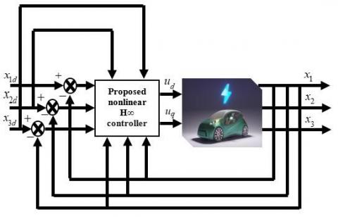
The applications of linear H∞ and Galerkin approximation approaches for nonlinear H∞ controllers in an EV powered by a PMSM given in (9) is described in this section. The control aim is to create a controller for an EV that is asymptotically stable and allows the d-axis current and EV speed to follow the reference signals. Figure 3 illustrates the overall scheme of the suggested controller.
Figure 3. The global EV driving system Block diagram
It is critical to convert the original nonlinear model provided in Eq. (9) into the associated error dynamics in order to develop the H-Infinity controllers for an Electric Vehicle Driven by the Permanent Magnet Synchronous Motor. The desired q-axis current, the speed error, the d-axis current error, and the q-axis current error can all be defined as [34, 35]:
$x_{e 1}=x_1-x_{1 d}, x_{e 2}=x_2-x_{2 d}, x_{e 3}=x_3-x_{3 d}$ (18)
$\begin{gathered}x_{2_{-} d}=\frac{2 J_{E V}}{3 P \Phi G_{\text {gear }}} \dot{x}_{3 \_d}+\frac{r_{\text {tire }}{ }^3 \rho A_f C_D}{3 J_{E V} P \Phi G_{\text {gear }}{ }^4} x_{3_{-} d}^2+ \frac{2 B G_{\text {gear }}}{3 P \Phi G_{\text {gear }} r_{\text {tire }}} x_{3_{-} d}+\frac{r_{\text {tire }}}{3 J_{E V} P \Phi G_{\text {gear }}{ }^2}(M g \sin (\alpha)+ \left.M g f_r \cos (\alpha)\right)\end{gathered}$ (19)
where, $x_{3_{-} d}$ is the desired speed, $x e_3$ is the speed error, $x e_1$ and $x e_2$ are, respectively, current errors.
$x_{1 \_d}$ and $x_{2 \_d}$ are the desired q-axis and d-axis currents respectively.
The control signals $u_{d_{-} s}$ and $u_{q_{-} s}$ can then be decomposed into the stabilizing and compensating terms listed below:
$u_d=u_{d_{-} s}+u_{d_{-} c}, u_q=u_{q_{-} s}-u_{q_{-} c}$ (20)
where, $u_{d_{-} c}$ and $u_{q_{-} c}$ are the d -axis compensating and stabilizing control terms, $u_{q_{-} c}$ and $u_{q_{-} s}$ are the q-axis compensating and stabilizing control terms, respectively.
$u_{d_{-} c}$ and $u_{q_{-} c}$, compensating control terms, are described as follows:
$u_{d_{-} c}=-\frac{L P G_{\text {gear }}}{r_{\text {tire }}} x_{2_{-} d} x_{3_{-} d}$ (21)
$u_{q_{-} c}=-\frac{L P G_{\text {gear }}}{r_{\text {tire }}} x_2 x_3$ (22)
The suggested linear and nonlinear H∞ controller is shown schematically in Figure 4.
Figure 4. The suggested linear and nonlinear H∞ controller schematic diagram
The following error dynamics can be used to express the vehicle dynamic model (18) to (22):
$\left\{\begin{array}{c}\dot{x}_{\mathrm{e} 1}=-\frac{R}{L} x_{e 1}+\frac{1}{L} u_{d_{-} s} \\ \dot{x}_{\mathrm{e} 2}=-\frac{R}{L} x_{e 2}-\frac{P \Phi G_{\text {gear }}}{L r_{\text {tire }}} x_{e 3}+\frac{1}{L} u_{q_{-} s} \\ \dot{x}_{\mathrm{e} 3}=\frac{1}{J_{E V}}\left[\frac{3 P \Phi G_{\text {gear }}}{2} x_{e 2}-\frac{\rho A_f C_D r_{\text {tire }}{ }^3}{2 G_{\text {gear }}{ }^3} x_{e 3}^2-\left(\begin{array}{c}\frac{B G_{\text {gear }}}{r_{\text {tire }}}+ \\ \frac{\rho A_f C_D r_{\text {tire }}{ }^3}{G_{\text {gear }}{ }^3} x_{3_{-} d}\end{array}\right) x_{e 3}\right]\end{array}\right.$ (23)
4.1 H∞ linear controller design
A linear system model is required for the Linear H-Infinity control design process. Therefore, in order to linearize the nonlinear Eq. (9) around its equilibrium point, Taylor's series expansion is used. The EV's linear state-space model is obtained as follows:
$\left\{\begin{array}{l}\dot{x}(t)=A_{x e} x(t)+B_{u_{-} s} u(t)+B_{w_{-} x e} w(t) \\ y=C_{x e} x(t)\end{array}\right.$ (24)
where, the state vector $x_e$ takes the forms of $x_e=$ $\left[x_{e 1}, x_{e 2}, x_{e 3}\right]^T ; u_{-} s$ represent the control input; $w_{-} x e$ represent the disturbance input of the system. The matrices $A_{x e}, B_{u_{-} s}, B_{w_{-} x e}$ and $C_{x e}$ of the state space model have the following definitions:
$\begin{gathered}A_{x e}=\left[\begin{array}{ccc}-\frac{R}{L} & 0 & 0 \\ 0 & -\frac{R}{L} & -\frac{P \Phi G_{g e a r}}{L r_{\text {tire }}} \\ 0 & \frac{1}{J_{E V}} \frac{3 P \Phi G_{g e a r}}{2} x_{e 2} & -\frac{1}{J_{E V}}\left(\begin{array}{c}\frac{B G_{\text {gear }}}{r_{\text {tire }}}+ \\ \frac{\rho A_f C_D r_{\text {tire }}{ }^3}{G_{\text {gear }}{ }^3} x_{3_d}\end{array}\right)\end{array}\right], \\ B_{u_{-} s}=\left[\begin{array}{l}\frac{1}{L} \\ \frac{1}{L} \\ 0\end{array}\right], B_{w_{-} x e}=\left[\begin{array}{l}1 \\ 1 \\ 0\end{array}\right], C_{x e}=\left[\begin{array}{lll}1 & 0 & 1\end{array}\right]\end{gathered}$ (25)
By resolving the associated Riccati equation, the following stabilizing state feedback control is obtained:
$\begin{aligned} & u_{d_{-} s L}\left(x_e\right)=-0.6897 x_{e 1}-0.6897 x_{e 2}+5.8621 x_{e 3} \\ & u_{q_{-} s L}\left(x_e\right)=-0.6897 x_{e 1}-0.6897 x_{e 2}+2.4138 x_{e 3}\end{aligned}$
4.2 H∞ nonlinear controller design
The successive Galerkin approximation technique for the Hamilton-Jacobi Isaacs equation was employed to develop a nonlinear H-Infinity controller for the EV powered by a PMSM system. We employed the initializing parameters, which are: the stability region Ω, the basic functions $\Phi(x)$ and an initial stabilizing linear $H \infty$ control $u^{(0)}(e)$.
The choice of the domain Ω is guided by the following conditions:
The system $\dot{x}=f(x)+g(x) u^{(0)}(x)$ must be asymptotically stable.
The domain Ω must be closed, continuous, and encompass the equilibrium point of the system.
In this paper, we used:
$\begin{gathered}\Omega=[1.2,1.2]^3 \\ \Phi=\left[x_{e 1}^2, x_{e 2}^2, x_{e 3}^2, x_{e 1} x_{e 2}, x_{e 1} x_{e 3}, x_{e 2} x_{e 3}\right] \\ u^{(0)}(e)=\left[u_{d_{-} s 0}\left(x_e\right), u_{q_{-} s 0}\left(x_e\right)\right]\end{gathered}$
where,
$\begin{aligned} & u_{d_{-} s 0}\left(x_e\right)=-0.6897 x_{e 1}-0.6897 x_{e 2}+5.8621 x_{e 3} \\ & u_{q_{-} s 0}\left(x_e\right)=-0.6897 x_{e 1}-0.6897 x_{e 2}+2.4138 x_{e 3}\end{aligned}$
γ takes an initial value of 520, its reduced value which ensures the algorithm convergence is chosen equal to 53. To find a suboptimal γ: Choose an initial control $u^{(0)}(x)$ and set γ. If the nonlinear H∞ problem is solvable, decrease γ and set $u^{(0)}(e)=u^{\infty}(e)$ (where $u^{\infty}(e)$ is the resulting control), then repeat step 1 (Algorithm 1). Otherwise, proceed to "Input: $u^{(0)}(x)$ an initial stabilizing control law, $\Omega$ stability region while increasing γ. The nonlinear H-Infinity control law that was obtained is given by:
$\begin{gathered}u_{d_{-} s_{-} N L}\left(x_e\right)=-0.9917 x_{e 1}-1.3104 e-18 x_{e 2}+2.3701 e-17 x_{e 3} \\ u_{q_{-} s_{-} N L}\left(x_e\right)=-1.3104 e-18 x_{e 1}-0.9917 x_{e 2}-0.0191 x_{e 3}\end{gathered}$
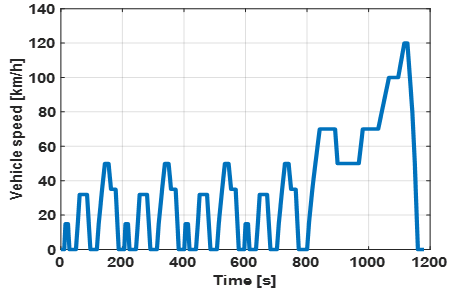
With the aim of evaluating the effectiveness of the EV powered by a PMSM, and to test the dynamic performance of linear H-Infinity control and Galerkin approximation approach for nonlinear H-Infinity control techniques. In this work, we adopt the NEDC (New European Driving Cycle) which is a standardized testing method developed by the European Union. It assesses vehicle fuel efficiency and emissions through a simulated driving profile that includes urban and extra-urban conditions. The cycle's structured approach, consisting of repeated driving phases, provides valuable data for comparing the environmental performance of different vehicles in controlled conditions. The NEDC is shown in Figure 5.
Figure 5. The new European driving cycle
The EV system's dynamic performances were compared using Matlab/Simulink. The tests are carried out under similar initial conditions to guarantee a fair and accurate comparison of the results using PMSM and EV parameters, which are shown in Tables 1 and 2 [36].
Table 1. Electrical parameters of the chosen PMSM
|
The Parameter |
Symbol |
Value |
Unit |
|
d-axis Inductances |
$L_{\mathrm{d}}$ |
0.29 |
mH |
|
q-axis Inductances |
$L_{\mathrm{q}}$ |
0.29 |
mH |
|
Flux linkage |
$\Phi$ |
0.071 |
wb |
|
Stator-winding resistance |
$R$ |
0.0083 |
Ω |
|
Number of poles |
P |
8 |
|
|
Moment of inertia |
J |
0.089 |
Kg.m2 |
|
Viscous friction coefficient |
B |
0.005 |
Nm/rad/s |
Table 2. The vehicle's specifications utilized in the simulation
|
The Parameter |
Symbol |
Value |
Unit |
|
Vehicle mass |
M |
1450 |
Kg |
|
Frontal area of the vehicle |
$A_f$ |
2.711 |
m2 |
|
Wheel radius |
$r_{\text {tire }}$ |
0.29 |
m |
|
Coefficient of aerodynamic drag |
$C_D$ |
0.29 |
|
|
Air density |
$\rho$ |
1.204 |
Kg/m3 |
|
Rolling resistance coefficient |
$f_r$ |
0.013 |
|
|
Total inertia |
|
5.209 |
Kg.m2 |
|
Total gear ratio |
$G_{\text {gear }}$ |
8.75 |
|
Figure 6. Electric vehicle speed under different control with NEDC driving cycle
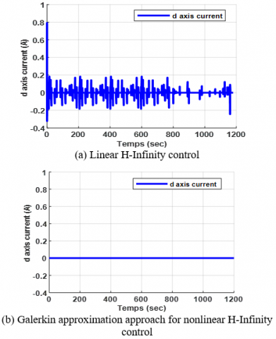
Figure 7. PMSM d-axis current with NEDC driving cycle under different control technique
Figure 6 illustrates the EV speed when the NEDC driving cycle is applied while using various control strategies. It is clearly visible that the vehicle’s speed tracking abilities are satisfactory; the vehicle reaches the reference speed with fast tracking performance, without any overshoot and zero steady state error.
Figure 7 depicts the response of the PMSM d-axis current by using the both control methods. It can be observed that the d-axis current responses rapidly follow the reference d-axis current for the duration of all low or high speed trajectories. The two approaches presented remarkable performance of tracking. Nevertheless, significant d-axis current ripples are observed in the case of linear H-Infinity control while the approach based on Galerkin approximation for nonlinear H-Infinity control strategies present unobservable ripples. That ripples in the d-axis current, particularly noticeable with the linear H-Infinity control approach, indicate a potential instability leading to undesirable variations in the motor's behaviour, there by affecting overall vehicle performance. These results show that the Galerkin approximation approach for nonlinear H-Infinity method gives better performance for the EV system during the NEDC cycle.
Figures 8 and 9 show q-axis current responses and electromagnetic torque of PMSM in the electric vehicle system using various control strategies. The q-axis current component is proportional to the torque component required, giving in dynamic response an excellent performance. To reach the different stages of the speed reference, the PMSM motor develop the necessary electromagnetic torque. It can be noticed that during all high- or low-speed trajectories, the torque responses closely match the varied speed values. These results demonstrate the effectiveness of the H-Infinity technique in the PMSM control systems.
Figure 8. PMSM q-axis current with NEDC driving cycle under different control technique
Figure 9. PMSM electromagnetic torque with NEDC driving cycle under different control technique
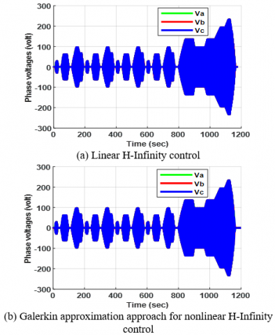
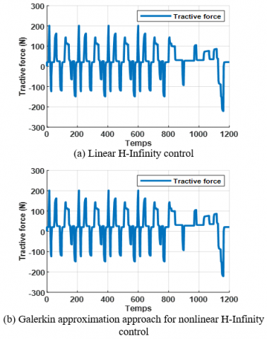
The phase voltages, phase currents, Tractive force, stator voltage components and traction power during the period of operation under the NEDC driving cycle for the linear H-Infinity and Galerkin approximation approach for nonlinear H-Infinity strategies are shown in Figures 10-13, respectively. It can be noticed that the phase voltages and phase currents are perfectly sinusoidal, their behavior as well as the frequency adapt as a result of the speed variation. The dynamic variation of tractive force and traction power corresponds to the changes of speed; the behavior of the tractive force is the same as that of the electromagnetic torques and traction power is shown as positive while power recovered during regenerative braking is negative. The shape of the stator voltage components depend on the reference speed.
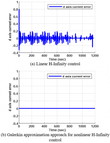
Figures 14 and 15 illustrate the speed tracking error and d axis current error in the H-Infinity and the nonlinear H-Infinity control strategies with Galerkin approximation approach, for several values of speed. It is obviously observed that the Galerkin approximation approach for nonlinear H-Infinity control technique significantly reduces the speed tracking error and d axis current error compared to the linear H-Infinity technique. Significant errors in these parameters can result in unstable driving and subpar motor performance. However, the Galerkin approach for nonlinear H-Infinity control strategies demonstrates a notable reduction in these errors compared to the linear H-Infinity approach. This improvement implies increased accuracy in speed and d-axis current tracking, contributing to enhanced system responsiveness and a smoother driving experience. Figure 16 illustrates the propulsion power of an electric vehicle during the NEDC cycle, showing positive power during acceleration and negative energy recovery during braking, suggesting energy efficiency in the vehicle's operation. These results validate the efficiency of the Galerkin approximation approach for nonlinear H-Infinity control technique for reducing tracking error and d axis current error in the control of the electric vehicle.
Figure 10. PMSM phase voltages waveform with NEDC driving cycle under different control technique
Figure 11. PMSM phase currents waveform with NEDC driving cycle under different control technique
Figure 12. Tractive force with NEDC driving cycle under different control technique
Figure 13. PMSM stator voltage components with NEDC driving cycle under different control technique
Figure 14. The speed tracking error with NEDC driving cycle under different control technique
Figure 15. D-axis current error with NEDC driving cycle under different control technique
Figure 16. Traction power with NEDC driving cycle under different control technique
In summary, the tests carried out through this section confirm that the Galerkin Approximation Approach for Nonlinear H-Infinity control technique significantly reduces the speed tracking error and d axis current error while also enhancing the quality of the d axis current. This approach also provides a faster dynamic response.
This work investigated an analysis in detail and a comparative study of two-control technique for an Electric Vehicle Powered by a Permanent Magnet Synchronous Motor. These two control strategies are the Linear H-Infinity and Galerkin approximation approach for Nonlinear H-Infinity, all designed and developed to meet vehicle needs. The simulation results were validated using numerical simulations in MATLAB/Simulink. The obtained results show that the Galerkin Approximation Approach for Nonlinear H-Infinity is the most efficient control strategy used to control the permanent magnet synchronous motor in an electric vehicle.
Comparing this strategy to the linear H-Infinity technique, it reduced the speed tracking error, decreased the PMSM's d axis current error, and gave a faster transient response. Therefore, the Galerkin Approximation Approaches for Nonlinear H-Infinity technique is a powerful candidate for electric vehicles powered by permanent magnet synchronous motor.
In upcoming work, we plan to investigate the solution to the Hamilton-Jacobi-Isaacs inequality equation arising in the Nonlinear H-Infinity problem with the assistance of an artificial intelligence technique (Reinforcement Learning).
The DG RSDT (Direction Générale de la Recherche Scientifique et du Développement Technologique) supported this work.
|
EV |
Electric Vehicle |
|
PMSM |
Permanent Magnet Synchronous Motor |
|
NEDC |
New European Driving Cycle |
[1] Schaltz, E., Soylu, S. (2011). Electrical vehicle design and modeling. Electric Vehicles-Modelling and Simulations, 1: 1-24. http://doi.org/10.5772/20271
[2] Mi, C., Masrur, M.A. (2017). Hybrid Electric Vehicles: Principles and Applications with Practical Perspectives. John Wiley & Sons.
[3] Salem, F.A. (2013). Modeling and control solutions for electric vehicles. European Scientific Journal, 9(15): 221-240.
[4] El Majdoub, K., Giri, F., Ouadi, H., Chaoui, F.Z. (2014). Nonlinear cascade strategy for longitudinal control of electric vehicle. Journal of Dynamic Systems, Measurement, and Control, 136(1): 011005. https://doi.org/10.1115/1.4024782
[5] Huang, Q., Huang, Z., Zhou, H. (2009). Nonlinear optimal and robust speed control for a light-weighted all-electric vehicle. IET Control Theory & Applications, 3(4): 437-444. https://doi.org/10.1049/iet-cta.2007.0367
[6] Makrygiorgou, J.J., Alexandridis, A.T. (2017). Fuzzy logic control of electric vehicles: Design and analysis concepts. In 2017 Twelfth International Conference on Ecological Vehicles and Renewable Energies (EVER), Monte Carlo, Monaco, pp. 1-6. https://doi.org/10.1109/EVER.2017.7935881
[7] Al-Jazaeri, A.O., Samaranayake, L., Longo, S., Auger, D.J. (2014). Fuzzy logic control for energy saving in autonomous electric vehicles. In 2014 IEEE International Electric Vehicle Conference (IEVC), Florence, Italy, pp. 1-6. https://doi.org/10.1109/IEVC.2014.7056100
[8] Tahami, F., Farhangi, S., Kazemi, R. (2004). A fuzzy logic direct yaw-moment control system for all-wheel-drive electric vehicles. Vehicle System Dynamics, 41(3): 203-221. https://doi.org/10.1076/vesd.41.3.203.26510
[9] Poornesh, K., Mahalakshmi, R., Jayadeep, S.R.V., Gunavardhan, R.N. (2022). Speed control of BLDC motor using fuzzy logic algorithm for low cost electric vehicle. In International Conference on Innovations in Science and Technology for Sustainable Development (ICISTSD), Kollam, India, pp. 313-318, https://doi.org/10.1109/ICISTSD55159.2022.10010397.
[10] Haddoun, A., Benbouzid, M., Diallo, D., Abdessemed, R., Ghouili, J., Srairi, K. (2006). Sliding mode control of EV electric differential system. In ICEM'06, Chania, Greece.
[11] Gair, S., Cruden, A., McDonald, J., Hredzak, B. (2004). Electronic differential with sliding mode controller for a direct wheel drive electric vehicle. In Proceedings of the IEEE International Conference on Mechatronics, Istanbul, Turkey, pp. 98-103. https://doi.org/10.1109/ICMECH.2004.1364419
[12] Mecifi, M., Boumediene, A., Boubekeur, D. (2021). Fuzzy sliding mode control for trajectory tracking of an electric powered wheelchair. AIMS Electronics and Electrical Engineering, 5(2): 176-193. https://doi.org/10.3934/electreng.2021010
[13] Saidi, K., Boumediene, A., Massoum, S. (2020). An optimal PSO-based sliding-mode control scheme for the robot manipulator. Elektrotehniski Vestnik, 87(1/2): 53-59.
[14] Roubache, T., Chaouch, S., Naït-Saïd, M.S. (2016). Backstepping design for fault detection and FTC of an induction motor drives-based EVs. automatika, 57(3): 736-748. https://doi.org/10.7305/automatika.2017.02.1733
[15] Bensalem, Y., Abbassi, A., Abbassi, R., Jerbi, H., Alturki, M., Albaker, A., Abdelkrim, M.N. (2022). Speed tracking control design of a five-phase PMSM-based electric vehicle: A backstepping active fault-tolerant approach. Electrical Engineering, 104(4): 2155-2171. https://doi.org/10.1007/s00202-021-01467-3
[16] Siffat, S.A., Ahmad, I., Ur Rahman, A., Islam, Y. (2020). Robust integral backstepping control for unified model of hybrid electric vehicles. IEEE Access, 8: 49038-49052. https://doi.org/10.1109/ACCESS.2020.2978258
[17] Zhang, C.W. (2010). Experiment of H∞ driving control system for electric vehicle. Applied Mechanics and Materials, 20: 215-219. https://doi.org/10.4028/www.scientific.net/AMM.20-23.215
[18] Boukhnifer, M., Chaibet, A., Ouddah, N., Monmasson, E. (2017). Speed robust design of switched reluctance motor for electric vehicle system. Advances in Mechanical Engineering, 9(11): 1687814017733440. https://doi.org/10.1177/1687814017733
[19] Khalil, I.S., Doyle, J.C., Glover, K. (1996). Robust and Optimal Control. Prentice Hall.
[20] Doyle, J., Glover, K., Khargonekar, P., Francis, B. (1988). State-space solutions to standard H2 and H∞ control problems. American Control Conference, Atlanta, GA, USA, pp. 1691-1696. https://doi.org/10.23919/ACC.1988.4789992
[21] Duc, G., Font, S. (1999). Commande H Infini et μ-Analyse des Outils Pour la Robustesse. Hermes Sciences Publications, Paris.
[22] Glover, K., Doyle, J.C. (1988). State-space formulae for all stabilizing controllers that satisfy an H∞-norm bound and relations to relations to risk sensitivity. Systems & Control Letters, 11(3): 167-172. https://doi.org/10.1016/0167-6911(88)90055-2
[23] Skogestad, S., Postlethwaite, I. (2005). Multivariable Feedback Control: Analysis and Design. John Wiley & Sons.
[24] Van Der Schaft, A.J. (1992). L2-gain analysis of nonlinear systems and nonlinear state feedback H∞ control. IEEE Transactions on Automatic Control, 37(6): 770-784. https://doi.org/10.1109/9.256331
[25] Van der Schaft, A. (2000). L2-Gain and Passivity Techniques in Nonlinear Control. Berlin, Heidelberg: Springer Berlin Heidelberg.
[26] Beard, R.W., Saridis, G.N., Wen, J.T. (1998). Approximate solutions to the time-invariant Hamilton–Jacobi–Bellman equation. Journal of Optimization theory and Applications, 96: 589-626. https://doi.org/10.1023/A:1022664528457
[27] Beard, R.W., Saridis, G.N., Wen, J.T. (1997). Galerkin approximations of the generalized Hamilton-Jacobi-Bellman equation. Automatica, 33(12): 2159-2177. https://doi.org/10.1016/S0005-1098(97)00128-3
[28] Bea, R.W. (1998). Successive Galerkin approximation algorithms for nonlinear optimal and robust control. International Journal of Control, 71(5): 717-743. https://doi.org/10.1080/002071798221542
[29] Guzzella, L., Sciarretta, A. (2013). Vehicle Propulsion Systems: Introduction to Modeling and Optimization. Springer-Verlag Berlin Heidelberg. https://doi.org/10.1007/978-3-642-35913-2
[30] Adegbohun, F., Von Jouanne, A., Phillips, B., Agamloh, E., Yokochi, A. (2021). High performance electric vehicle powertrain modeling, simulation and validation. Energies, 14(5): 1493. https://doi.org/10.3390/en14051493
[31] Husain, I. (2021). Electric and Hybrid Vehicles: Design Fundamentals. 3rd ed. Boca Raton: CRC Press. https://doi.org/10.1201/9780429490927
[32] Genta, G. (1997). Motor vehicle dynamics: Modeling and simulation. Series on Advances in Mathematics for Applied Sciences, Vol. 43. World Scientific.
[33] Attia, M., Zaamouche, F., Houam, A., Daouadi, R. (2022). Stability control modeling and simulation strategy for an electric vehicle using two separate wheel drives. European Journal of Electrical Engineering, 24(5-6): 239-245. https://doi.org/10.18280/ejee.245-602
[34] Do, T.D., Choi, H.H., Jung, J.W. (2011). SDRE-based near optimal control system design for PM synchronous motor. IEEE Transactions on Industrial Electronics, 59(11): 4063-4074. https://doi.org/10.1109/TIE.2011.2174540
[35] Do, T.D., Choi, H.H., Jung, J.W. (2015). θ-D approximation technique for nonlinear optimal speed control design of surface-mounted PMSM drives. IEEE/ASME Transactions on Mechatronics, 20(4): 1822-1831. https://doi.org/10.1109/TMECH.2014.2356138
[36] Oudjama, F., Boumediene, A., Saidi, K., Boubekeur, D. (2023). Robust speed control in nonlinear electric vehicles using H-infinity control and the LMI approach. Journal of Intelligent Systems and Control, 2(3): 170-182. https://doi.org/10.56578/jisc020305