Chinedu A. K. Ezugwu*![]() | Ojo S. I. Fayomi
| Ojo S. I. Fayomi![]() | Morakinyo K. Onifade
| Morakinyo K. Onifade![]() | Adeyinka O. M. Adeoye
| Adeyinka O. M. Adeoye![]() | Imhade P. Okokpujie
| Imhade P. Okokpujie![]()
© 2023 IIETA. This article is published by IIETA and is licensed under the CC BY 4.0 license (http://creativecommons.org/licenses/by/4.0/).
OPEN ACCESS
Machining is fundamentally a process of material removal. Therefore, machining productivity can be conceptualized as the rapid elimination of a substantial machining allowance, implying a reduction in machining time. This research has yielded a computational model predicated on beam deflection, factoring in the influence of workpiece flexibility on cutting forces, and its repercussions on the material removal rate and precision. The model facilitates the calculation of actual turning productivity. The methodology incorporated modeling the static response of the flexible workpiece to the thrust component of cutting forces. The impacts of flexibility on the beam model responses concerning the material removal rate, and deviations from the desired shape and size were scrutinized. A computational approach, experimentally corroborated, was applied. This approach necessitates cutting force coefficients, which were ascertained through cutting tests and pseudo-inverse regression analysis. The experimental setup for the cutting test incorporated a locally constructed dynamometer for measuring cutting forces, displays on both an LCD and a computer monitor for recording cutting force readings, a cutting tool, and a workpiece. Judging by the coefficients of determination, R2 values of 0.97, 0.89, and 0.93 of the regression calibrating the force coefficients for the tangential, feed, and radial directions-which are used to gauge the accuracy of the determined force coefficient and are typically one or close to one-the derived force coefficients demonstrate high reliability. The developed model is projected to yield significant industrial-economic benefits by curtailing the costs of finishing operations on the CNC lathe machine, owing to the provision of a chronological path to follow while working on a flexible workpiece.
beam model, cutting force, force coefficients, machining accuracy, material removal rate, workpiece flexibility, turning
Machining is a material removal process. In light of this, it is important to think of machining productivity as the quick removal of a large amount of machining allowance, which suggests a shorter machining time. The machining process has since advanced from conventional methods to the present-day where a computer is used to numerically control the machining activities which is adjudged as the core of manufacturing industries [1, 2]. The influence of machining parameters of turning process on the material removal rate under dry cutting conditions was considered [3, 4]. Workpiece of ±30° filament wound glass fibre reinforced polymers (GFRP) was of great interest in the work with cutting tool coated with tungsten carbide inserts. Regression analysis and factorial experimental design were employed to develop a second-order empirical model at a confidence interval of 95% for the material removal rate of the machining process. The empirical model was used to generate contour plots of the material removal rate for different machining conditions in the form of iso-value of roughness for diverse values of material removal rate. The optimization of the Material Removal Rate with turning process of EN24 steel were presented [5]. Independent adjustments of the cutting process parameters were the basis for the optimization. The rate of metal removal was optimized on the larger-the-better basis. In the works [6, 7], the effects of the cutting process parameters on material removal rate in turning of C34000 were presented as a solitary response optimization problem solved by using Taguchi technique. Twenty-seven experimental runs were performed focusing on L’27 orthogonal array with the aim of optimizing the objective functions within the experimental domain formed. The work led to the determination of the optimum choices of process parameters for the optimization of MRR and experimental confirmation of the optimal choices was implemented. In order to identify pertinent energy efficiency and productivity KPIs of machining processes, Hacksteiner et al. [8] used an approach based on a real-time analysis of sensor data and machine control data. This work obtained the energetic efficiency and the primary processing time by comparing the energetic model of the load-free condition with the machining power consumption. To validate the developed approach, a CNC turning and milling centers were used to automatically calculate some KPIs, SCADA software reads, processes, and records sensor data along with pertinent machine control data. Eberspächer et al. [9] considered approaches which monitored power consumptions and to reduce the power consumption. This work considered a machine control data read via OPC UA and additional sensor data which were considered as an input for the consumption simulation models to make available the detailed power consumption and distribution data for the machine operators. Hu et al. [10], developed a special on-line system for energy efficiency monitoring of machine tools. This approach relied on the spindle power measurement based on power balance calculations. New approach that focused on optimizing the machining process for face milling of Stainless steel 316 under various cooling and lubrication strategies was developed by Abbas et al. [11]. The suggested strategy takes into account three process designs (balanced, cost, and quality-oriented designs). Using a vector regression model, experimental runs were designed which later became an objective function for the particle swarm optimization algorithm. This study advised using MQL and faster cutting speeds in all designs. While it was considered that higher feed rates were favoured in a quality-oriented design over a cost-oriented one. This analysis uses this method to create many designs, each biased toward one of the replies, in addition to offering an adaptive design. Bagaber and Yusoff [12] in their research used response surface method (RSM) and desirability function for stainless steel 316 turning optimization. The tools used were carbide coated and were deployed in various dry machining conditions to aid in minimizing power consumption, machined surface roughness and tool wear. Also, using a regression model, with an R2 less than 0.88, the three responses were modeled. This work only considered a case having equal weight while the compound desirability function was then formulated. In addition, this work selected a solution with a desirability function of 0.887 for the final optimum solution. Thus, the work reported a reduction in the tool wear, energy consumption and the machined surface roughness by 4.71, 14.94 and 13.89%, respectively. Abbas et al. [13] investigated the precision hard turning of AISI 4340 alloy steel using wiper nose and common round nose inserts. It tries to identify the best process variables for reducing surface roughness and increasing productivity at the same time and gives readers a closer look at earlier studies. Surface roughness at different cutting speeds, depths of cut, and feed rates is treated as the target function in the mathematical models created by the authors. The optimal turning parameters were determined using three reliable multi-objective methods: the multi-objective genetic algorithm (MOGA), the multi-objective Pareto search algorithm (MOPSA), and the multi-objective emperor penguin colony algorithm (MOEPCA). Two turning scenarios were employed to assess the effectiveness of the optimization methods. In these, a gun barrel's combustion chamber was machined at a high rate of production, initially with an average roughness (Ra) of 0.4 m and thereafter with 0.8 m. This work shows that MOPSA is the best appropriate option for the wiper insert scenario and that MOEPCA results are the best for the traditional insert in order to concurrently achieve good surface quality and productivity in precision hard turning of AISI 4340 alloy steel. Also, the results of the Pareto front plot demonstrate that the wiper insert may achieve good productivity and Ra values of 0.4 and 0.8. However, the conventional insert proved unable to achieve the required 0.4 m Ra; instead, Ra=0.454 m was observed globally, demonstrating the wiper's superiority to the conventional insert. Yan and Li [14] also carried out optimization for a milling process. This work considered three different responses which are; surface roughness, material removal rate and cost. Relying on grey relation analysis (GRA), trade-off in turning parameters (speed, feed, and depth of cut) was managed. This work proposed that weights assignment should be based on the sensitivity of each of the response to the turning parameters. Thus, this work selected weights of 0.33, 0.23, and 0.43 for the surface roughness, material removal rate and cost. They reported that the proposed approach was effective in terms of cost and suggested that the conventional one was preferred when considering surface roughness. Although, they noted that both approaches showed similar material rate removals. Chandrasekhar and Prasad [15] carried out optimization for micro-drilling operation. Employing Entropy-VIKOR method in their approach, weights were selected based on the disorder degree which was coined from Shannon entropy method. The challenges were reduced to a single objective using the weights of the VIKOR approach, and the best solution was thought to have the highest VIKOR rank. Only the weights from the entropy approaches were considered in their procedure. A machining assessment model that focused on five parameters-energy, safety, cost, environmental impact, health, and waste management-was developed by Hegab et al. [16] in their study. To account for different requirements and intentions, the model assigned weights. Three case studies from their literature were used in this work to test the proposed paradigm. This method helped to make optimal predictions that are compatible with the optimums reported in the original experimental work since equal weights were given to all of the analyzed cases. In order to forecast the productivity of the sinter machine using the composition of the agglomerate's constituent elements as model inputs, Mallic et al. [17] employed machine learning and data analytics techniques. An integrated steel plant provided them with industrial productivity statistics for the sinter machines. According to this study, the proposed ANN model was significantly compatible with the productivity of the sinter machine as tested. The sensitivity analysis further revealed that the proportions of MgO and CaO present in flux and sinter, respectively, have a substantial impact, but the presence of iron (Fe) and SiO2 in iron ore fines and sinter has a positive effect on sinter machine productivity. Wei et al. [18] in their work reported a different approach for high power and high-speed density laser-assisted turning (LAT) of an Al-SiC MMC (Al2124+17 vol% 0.3 μm SiC). They opined that this approach greatly improve productivity by allowing parts to be removed from the surface of the locally heated parts to be removed timely while avoiding transfer of excess heat from the surface to the main body. They further reported a smaller laser beam diameter of 0.7 mm as compared to the nose radius of the turning insert of 0.8 mm which was noted to aid the removal of the excess heat generated from the laser radiation from the chips. Results show a laser power density of 3.38 × 10⁶ W/cm2 was used which they noted to be twice higher than those reported in previous LAT research. In addition, a cutting speed of 565 m/min produced over 2.7–140 times increase in productivity compared with previously reported values, and the surface quality was substantially improved in addition to reduced tool wear. Understanding the performance of three distinct industrial-grade CBN cutting inserts during hard turning of AISI 4320 case-carburized steel was the main goal of the work by Niaki et al. [19]. Although all the CBN inserts were found to have the same shape, they all had various edge preparation and coating techniques. While the surface integrity of the machined item was described based on the surface roughness, layer depths, micro-hardness, and residual stresses, this work quantified the tool performances by measuring the cutting forces and tool wear at frequent intervals. Finally, their findings showed that the cutting-edge stability of tested inserts influences tool life, cutting force stability, and the development of compressive residual stresses on the surface of the turned workpiece. Moreover, Camposeco-Negrete and de Dios Calderón-Nájera [20] used multi-objective optimization to increase the productivity, energy efficiency, and surface quality of turning AISI 6061 T6 aluminum. Power consumption and surface roughness were optimized simultaneously by Sangwan and Kant [21]. Surface roughness, however, is a fixed characteristic rather than a variable in the machining process (predefined range by designers). Surface roughness that is less than the intended value is typically acceptable but not necessary [22]. In the work Khan et al. [23], turning experiments were explored to analyze the productivity and machining efficiency in the machining sustainability of Ti-6Al-4V alloy. In the experiment, cutting time was considered fixed while the cutting speed kept high in the hybrid CryoMQL (HCM) method. Comparative results were recorded in all the experiments performed in different cooling techniques. Further results on the comparison between the methods showed that the HCM method performed better than dry and MQL method. This work opined that the proposed method would provide longer tool life, lower energy consumption and higher productivity. Also, proposed technology can enhance high productivity and save cost in metal processing industry to get. Pang et al. [24] investigated end milling process on hybrid composite of hallo site nanotubes and carried out the optimization process of the parameters by using Taguchi method. The input factors considered in this work includes; feed, speed and depth of cut. The input factors were mentioned to help study the cutting force and surface finish. Ribeiro et al. [25] in their work on optimization of surface roughness considered axial and radial depths as part of their input parameters list. Using ANOVA and orthogonal arrays to study the parameters influences observed that radial and axial depth plays a significant role in the improved finishing on milling.
This research aims to develop a computational model that takes into account the impact of workpiece flexibility on cutting forces, as well as how these factors affect the rate of material removal and machining precision so as to reduce the cost of working on flexible workpiece while maintaining the integrity of the end product. The focus was on the limitation to material removal rate due to the consideration of the flexibility of slender workpieces machined by turning process. Therefore, the cutting force component causing workpiece deflection in the thrust direction is of interest in this work thus was modelled. The emphasis was on the cases of CNC lathe operations where the workpieces was modelled as rotating fixed-pinned beams due to fixed supports at the chucks and pinned supports at the tailstock centres. The cases of CNC lathe operations where the workpieces were modelled as rotating fixed-free (cantilevered) beams due to fixed supports at the chucks and unsupported end on the other sides of the workpieces was not considered in this work. The technique involves simulating the flexible workpiece's static reaction to the thrust component of cutting forces. The impacts of flexibility on the beam models' responses to the rate of material removal and the degree of divergence from the planned size and shape were investigated. The method was computational and empirically tested. With the help of this model, the actual turning productivity may be calculated thereby reducing the costs of finishing operation of the CNC lathe machine because a chronological path to follow while working on flexible workpiece has been provided.
Machining productivity is quantified in terms of machining time, material removal rate, and machining economics. Basically, the complete machining time or total time for machining (Tm), is the addition of all the three separate unrelated components of time that directly relate with the process of machining.
The time components are listed below;
Arithmetically, the complete Time for Machining (Tm) may be expressed as:
$\mathrm{T}_{\mathrm{m}}=\mathrm{T}_{\mathrm{ct}}+\mathrm{T}_{\mathrm{i}}+\mathrm{T}_{\mathrm{c}}$ (1)
Let s be the rate of feed (mm/rev), Lc be the complete cut length (mm), and Ω be the speed of the spindle (rpm), then proposed cutting time may be articulated as:
$\mathrm{T}_{\mathrm{c}}=\frac{L_c}{\Omega \cdot s}$ (2)
Conventionally, at the point when the workpiece or the cutting instrument is in pivot, speed of the spindle and speed of cut ( Vc ) are interchangeable. This is on the grounds that it is expected that there is no loss of speed from the spindle speed or the workpiece's speed for the cutting speed. Nonetheless, cutting speed likewise relies upon the measurement of the job/cutter (D). Based on this, we can communicate the cutting speed as a function of diameter as below:
$V_c=\frac{\pi D \Omega}{1000}$ (3)
Then,
$\mathrm{Tc}=\frac{L_s}{\Omega . s}=\frac{L}{\left(\frac{1000 V_c}{\pi D}\right) s}=\frac{\pi D L}{1000 V_c s}$ (4)
The Expression for Taylor’s Tool Life is
$\mathrm{V}_{\mathrm{S}}(\mathrm{TL})^{\mathrm{n}}=\mathrm{C}$ (5)
$\mathrm{TL}=\left(\frac{C}{V_c}\right)^{1 / n}$ (6)
Meanwhile complete machining adjustment time (Tct) likewise relies upon the extent of adjustments desires, so device life will impact this time component. In this way, in the event that TCT be the time needed for single instrument changing, complete machining adjustment time (Tct) for the whole machining activity of $T_{c t}$ length can be communicated as below:
$T_{c t}=\frac{T_c}{T L} * T C T$ (7)
Therefore, the complete machining time or total time for machining may be articulated as below:
$\mathrm{T}_{\mathrm{m}}=\mathrm{T}_{\mathrm{ct}}+\mathrm{T}_{\mathrm{i}}+\mathrm{T}_{\mathrm{c}}$ (8)
$\mathrm{Tm}=\mathrm{Tc}+\frac{T_C}{T L} * T C T+\mathrm{T}_{\mathrm{i}}$ (9)
$\mathrm{Tm}=\frac{\pi D L}{\left(1000 V_c\right) s}+\left\{\frac{\frac{\pi D L}{\left(1000 V_C\right) s}}{\left(\frac{C}{V_c}\right)^{1 / n}} \times T C T\right\}+\mathrm{T}_{\mathrm{i}}$ (10)
$\mathrm{T}_{\mathrm{m}}=\frac{\pi D L}{\left(1000 V_c\right) s}+T C T \frac{\pi D L}{1000 s C^{1 / n}} V_c^{\frac{1-n}{n}}+T_i$ (11)
The actual machining time is of interest in this work. In several works, the actual machining time is considered a predictor of surface integrity and material removal rate rather than an objective. Qehaja et al. [26] considered surface roughness (Ra) as a response to machining parameters, such as depth of cut, nose radius, true rake angle, cutting speed, machining time, feed rate, side cutting edge angle. Exploiting response surface methodology focused on three-level factorial design, they instituted an empirical model for surface roughness in terms of the machining parameters like the tool geometry, machining time, nose radius, and feed rate in the course of dry turning process. Their statistical analysis showed that machining time is a significant factor.
Figure 1. The cutting force system
In Figure 1 is shown the cutting force $R$. The force $F_c$ is the tangential cutting force component while force $N_c$ is the feed cutting force component. The force $F_{s p}$ is the shear force component on the shear plane while force $N_{s p}$ is the normal force component on the shear plane. The force $F_{r f}$ is the frictional force component on the rake face of the tool while force $N_{r f}$ is the normal force component on the rake face. The important angles are also indicated as $\alpha$ for rake angle, $\varphi$ for shear angle and $\beta$ is the friction angle. The following equations, which are obvious from the geometry of Figure 1 , hold for the forces [27, 28].
$F_{s p}=F_c \cos \varphi-N_c \sin \varphi$ (12)
$N_{s p}=F_c \sin \varphi+N_c \cos \varphi$ (13)
$r_{c h}=\frac{h}{h_{c h}}=\frac{\sin \varphi}{\cos (\varphi-\alpha)}$ (14)
$\varphi=\tan ^{-1}\left(\frac{r_{c h} \cos \alpha}{1-r_{c h} \sin \alpha}\right)$ (15)
$F_{r f}=F_c \sin \alpha+N_c \cos \alpha$ (16)
$N_{r f}=F_c \cos \alpha-N_c \sin \alpha$ (17)
$\beta=\alpha+\tan ^{-1}\left(\frac{N_c}{F_c}\right)$ (18)
$V_{c h}=r_{c h} V_t$ (19)
where $r_{c h}$ is called chip compression ratio which is the thickness of metal before cutting to the thickness of metal after cutting and it is always less than one in the form defined, h is the undeformed chip thickness, $h_{c h}$ is the chip thickness which is the measurement of the material's thickness taken immediately before it is machined, perpendicular to the cutting edge and $h_{c h}$ is the chip velocity on the rake face. The speed of the chip as it travels along the tool face and in relation to the tool is known as chip velocity. From the above equations and the geometry of the cutting force system, it can be seen that
$N_{s p}=\frac{h w}{\sin \varphi} \sigma_{s p}=\frac{N_c}{\sin \phi} \sin (\varphi+\phi)$ (20)
where $\sigma_{s p}$ is the yield normal stress of the material and $w$ is the depth of cut. Therefore, the feed force component becomes
$N_c=\left[\sigma_{s p} \frac{\sin \phi}{\sin \varphi \sin (\varphi+\phi)}\,\,\right] h w$ (21)
Noting that $\phi=\beta-\alpha$, then
$N_c=\left[\sigma_{s p} \frac{\sin (\beta-\alpha)}{\sin \varphi \sin (\varphi+\beta-\alpha)}\,\,\right] h w$ (22)
Also, from the above equations and the geometry of the cutting force system, it can be seen that
$F_{s p}=\frac{h w}{\sin \varphi} \tau_{s p}=\frac{N_c}{\sin \phi} \cos (\varphi+\phi)$ (23)
where $\tau_{s p}$ is the yield shear stress of the material. Yield stress is the lowest stress at which a solid will permanently deform or flow into a different shape without significantly increasing the load or external force. Therefore, the feed force component can also be written as
$N_c=\left[\tau_{s p} \frac{\sin \phi}{\sin \varphi \cos (\varphi+\phi)}\,\,\right] h w$ (24
This is the same as
$N_c=\left\lceil\tau_{s p} \frac{\sin (\beta-\alpha)}{\sin \varphi \cos (\varphi+\beta-\alpha)}\,\,\right\rceil h w$ (25)
Since the two expressions for Nc are equivalent then
$\frac{\sigma_{s p}}{\sin (\varphi+\beta-\alpha)}=\frac{\tau_{s p}}{\cos (\varphi+\beta-\alpha)}$ (26)
giving the relationship between the two yield stresses as
$\sigma_{s p}=\tau_{s p} \tan (\varphi+\beta-\alpha)$ (27)
For same workpiece-tool pair $r_{c h}$ can be considered fixed meaning that $\varphi$ can also be considered fixed. The ratio $\frac{N_c}{F_c}$ is normally considered fixed for same workpiece-tool pair meaning that $\beta$ can be considered fixed and the yield stresses are fixed material properties. The deduction is therefore that the feed force component $N_c$ is proportional to the undeformed chip cross-section $h w$ where the constant of proportionality is either given as
$K_f=\sigma_{s p} \frac{\sin (\beta-\alpha)}{\sin \varphi \sin (\varphi+\beta-\alpha)}$ (28)
Or
$K_f=\tau_{s p} \frac{\sin (\beta-\alpha)}{\sin \varphi \cos (\varphi+\beta-\alpha)}$ (29)
Similar analyses give
$F_c=\left[\sigma_{s p} \frac{\cos (\beta-\alpha)}{\sin \varphi \sin (\varphi+\beta-\alpha)}\,\,\right] h w$ (30)
$F_c=\left[\tau_{s p} \frac{\cos (\beta-\alpha)}{\sin \varphi \cos (\varphi+\beta-\alpha)}\,\,\right] h w$ (31)
$K_t=\sigma_{s p} \frac{\cos (\beta-\alpha)}{\sin \varphi \sin (\varphi+\beta-\alpha)}$ (32)
$K_t=\tau_{s p} \frac{\cos (\beta-\alpha)}{\sin \varphi \cos (\varphi+\beta-\alpha)}$ (33)
where it is seen that
$K_f=K_t \tan (\beta-\alpha)$ (34)
The maximum shear stress theories of Krystof, Ernst and Merchant, and Stabler give [29, 30]
$\varphi=\frac{\pi}{4}-\beta+\alpha$ (35)
$\varphi=\frac{\pi}{4}-\frac{(\beta-\alpha)}{2}$ (36)
$\varphi=\frac{\pi}{4}-\beta+\frac{\alpha}{2}$ (37)
These equations are useful for the determination of the friction angle. Qiu [28] has reported that the thrust force which is radial in the case of turning can be given as
$F_{t h}=K_{t h} h w$ (38)
where the thrust force coefficient $K_{t h}$ is given as
$K_{t h}=K_t \tan (\beta-\alpha)$ (39)
This translates to the two equations
$K_{t h}=\sigma_{s p} \frac{\sin (\beta-\alpha)}{\sin \varphi \sin (\varphi+\beta-\alpha)}$ (40)
$K_{t h}=\tau_{s p} \frac{\sin (\beta-\alpha)}{\sin \varphi \cos (\varphi+\beta-\alpha)}$ (41)
During machining, there is a rubbing of the machined surface on the flank edge of the tool. The rubbing force is proportional to the depth of cut, therefore, the measured forces are more appropriately given as
$F_{c, s u m}=K_t h w+K_{t, e} w$ (42)
$N_{c, s u m}=K_f h w+K_{f, e} w$ (43)
$F_{t h, s u m}=K_{t h} h w+K_{t h, e} w$ (44)
where the edge force coefficients; $K_{t, e}, K_{f, e}$ and $K_{t h, e}$ are the edge rubbing force coefficients which are measured experimentally. The coefficients are normally read-off the graph of force against chip thickness as intercept per depth of cut. Also, Qiu [28] reported that the edge thrust force which is radial in the case of turning can be given as
$K_{t h, e}=K_{t, e} \tan (\beta-\alpha)$ (45)
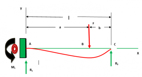
Figure 2. The fixed-pinned beam deflection model of a slender workpiece supported by the chuck and the tailstock centre
The methods involve modelling the static response of the flexible workpiece to the thrust component of cutting forces. The separate cases considering the workpiece as a cantilever and fixed-pinned beams was modelled and the effects of the responses of the beam-models on the material removal rate, and the extent of deviation from the intended shape and size was studied. The equations for the deflections of the fixed-pinned beam as depicted in Figure 2 (which is the appropriate model for a flexible workpiece supported by the chuck and the tailstock centre are [31, 32]. With the knowlede of the equations in section three (3), the needed computational model was derived.
$R_1=\frac{F b}{2 l^3}\left(3 l^2-b^2\right)=V_{A B}$ (46)
$R_2=\frac{F a^2}{2 l^3}(3 l-a)=-V_{B C}$ (47)
$M_1=\frac{F b}{2 l^2}\left(b^2-l^2\right)$ (48)
$M_{A B}=\frac{F b}{2 l^3}\left(b^2 l-l^3-x\left(3 l^2-b^2\right)\right)$ (49)
$M_{B C}=\frac{F a^2}{2 l^3}\left(3 l^2-3 l x-a l+a x\right)$ (50)
$y_{A B}=\frac{F b x^2}{12 E I l^3}\left(3 l\left(b^2-l^2\right)+x\left(3 l^2-b^2\right)\right)$ (51)
$y_{B C}=y_{A B}-\frac{F(x-a)^3}{6 E I}$ (52)
The equations for the deflections of the cantilever beam as depicted in Figure 3 which is the appropriate model for a slender workpiece supported by the chuck alone are [31, 32].
Figure 3. The cantilever beam deflection model of a slender workpiece supported by the chuck alone
$R_1=V=F$ (53)
$M_1=-F a$ (54)
$M_{A B}=F(x-a)$ (55)
$M_{B C}=0$ (56)
$y_{A B}=\frac{F x^2}{6 F I}(x-3 a)$ (57)
$y_{B C}=\frac{F a^2}{6 E I}(a-3 x)$ (58)
These equations were then transformed to represent the machining problem under consideration. Using these equations, this research unravelled the influence of workpiece flexibility on cutting forces and the effects on material removal rate and accuracy.
The determination of the cutting force coefficients requires a variation of the factors $v$ while keeping $w$ and $\Omega$ constant. The corresponding values of $h$ were calculated from $v$ and $\Omega$ where $h=60 v \cos \vartheta / \Omega$. In determining the cutting force coefficients, the effects of flexibility were excluded by using nonflexible workpiece and tool.
If the adopted experimental plan requires n runs, then the set of equations become
$\begin{gathered}F_{t h, s u m, 1}=K_{t h} w h_1+K_{t h, e} w \\ F_{t h, s u m, 2}=K_{t h} w h_2+K_{t h, e} w \\ \vdots \\ F_{t h, s u m, n}=K_{t h} w h_n+K_{t h, e} w\end{gathered}$ (59)
The linear system of equations can be put in matrix form as
$\mathbf{y}=w \mathbf{X c}$ (60)
The coefficients therefore become
$\mathbf{c}=\frac{1}{w}\left\{\mathbf{X}^{\mathrm{T}} \mathbf{X}\right\}^{-1} \mathbf{X}^{\mathrm{T}} \mathbf{y}$ (61)
where $\mathbf{c}$ is a 2 by 1 matrix of coefficients given as any of the three equations for the tangential, feed and thrust components.
$\mathbf{c}_{F_{c, s u m}}=\left\{\begin{array}{c}K_t \\ K_{t, e}\end{array}\right\}$ (62)
$\mathbf{c}_{N_{c, s u m}}=\left\{\begin{array}{c}K_f \\ K_{f, e}\end{array}\right\}$ (63)
$\mathbf{c}_{F_{t h, s u m}}=\left\{\begin{array}{c}K_{t h} \\ K_{t h, e}\end{array}\right\}$ (64)
$\mathbf{X}$ is an $n$ by 2 matrix of the factors given as
$\mathbf{X}=\left\{\begin{array}{cc}h_1 & 1 \\ h_2 & 1 \\ \vdots & \vdots \\ h_n & 1\end{array}\right\}$ (65)
$\mathbf{y}$ is an $n$ by 1 matrix of responses given as any of the three equations for the tangential, feed, and thrust components.
$\mathbf{y}_{F_{c, \text { sum }}}=\left\{\begin{array}{c}F_{c, \text { sum }, 1} \\ F_{c, \text { sum }, 2} \\ \vdots \\ F_{c, \text { sum }, n}\end{array}\right\}$ (66)
$\mathbf{y}_{N_{c, \text { sum }}}=\left\{\begin{array}{c}N_{c, \text { sum }, 1} \\ N_{c, \text { sum }, 2} \\ \vdots \\ N_{c, \text { sum } n}\end{array}\right\}$ (67)
$\mathbf{y}_{F_{\text {th }, \text { sum }}}=\left\{\begin{array}{c}F_{\text {th,sum }, 1} \\ F_{t h, \text { sum }, 2} \\ \vdots \\ F_{\text {th }, \text { sum } n}\end{array}\right\}$ (68)
The graphical plots and various error indices like the coefficient of determination $\mathrm{R}^2$, root mean square error RMSE, Mean biased error MBE, Mean absolute biased error MABE, Mean percentage error MPE as expressed below was used to evaluate the adequacy of the calibrated force coefficients.
$\mathrm{R}^2=1-\frac{\sum_{i=1}^n\left(T_i-y_i\right)^2}{\sum_{i=1}^n\left(T_i-\bar{y}\right)^2}$ (69)
$\operatorname{RMSE}=\left(\frac{1}{n} \sum_{i=1}^n\left(y_i-T_i\right)^2\right)^{0.5}$ (70)
$\mathrm{MBE}=\frac{1}{n} \sum_{i=1}^n\left(y_i-T_i\right)$ (71)
$\mathrm{MABE}=\frac{1}{n} \sum_{i=1}^n\left|\left(y_i-T_i\right)\right|$ (72)
$\mathrm{MPE}=\frac{1}{n} \sum_{i=1}^n\left(\frac{y_i-T_i}{T_i}\right) 100$ (73)
In the equations, y represents the predicted values while T represents the experimental values.
The methodology established above was used in determining the cutting force coefficients. The setup shown in Figure 4 was used. The setup is made up of a locally constructed dynamometer for measuring cutting forces, displays on both LCD and computer monitor, a cutting tool, and a workpiece. The Experimental matrix for determination of force coefficients was then completed as shown in Table 1. The entries are averages of the sampled values.
Figure 4. Experimental setup for determining force coefficients
Table 1. Experimental cutting force components values
|
Feed Speed $v[\mathrm{~m} / \mathrm{s}]$ |
Feed $h[\mathrm{~m} / \mathrm{rev}]$ |
Tangential Force $F_{c, \text { sum }}[\mathrm{N}]$ |
Feed Force $N_{c, \text { sum }}[\mathrm{N}]$ |
Thrust Force $F_{t h, s u m}[\mathrm{~N}]$ |
|
0.001 |
0.0002 |
56.84 |
36.93 |
17.19 |
|
0.002 |
0.0004 |
68.15 |
42.19 |
21.31 |
|
0.003 |
0.0006 |
87.36 |
65.17 |
26.12 |
|
0.004 |
0.0008 |
120.91 |
67.91 |
45.70 |
|
0.005 |
0.001 |
146.38 |
72.07 |
53.05 |
Using Eq. (61), the vector of coefficients for the tangential, feed and thrust cutting force components are $K_{t h}=4.5245 \times 10^8 \mathrm{Nm}^{-2}$ and $K_{\text {the }}=0.0005 \times 10^8 \mathrm{Nm}^{-1}$.
$\begin{gathered}\mathbf{c}_{F_{c, \text { sum }}}=\left\{\begin{array}{c}K_t \\ K_{t, e}\end{array}\right\}=\left\{\begin{array}{l}2.32 \times 10^8 \mathrm{Nm}^{-2} \\ 5.27 \times 10^4 \mathrm{Nm}^{-1}\end{array}\right\} \\ \mathbf{c}_{N_{c, \text { sum }}}=\left\{\begin{array}{c}K_f \\ K_{f, e}\end{array}\right\}=\left\{\begin{array}{l}9.60 \times 10^7 \mathrm{Nm}^{-2} \\ 5.61 \times 10^4 \mathrm{Nm}^{-1}\end{array}\right\} \\ \mathbf{c}_{F_{\text {th sum }}}=\left\{\begin{array}{c}K_{t h} \\ K_{\text {th }, e}\end{array}\right\}=\left\{\begin{array}{l}9.61 \times 10^7 \mathrm{Nm}^{-2} \\ 7.68 \times 10^3 \mathrm{Nm}^{-1}\end{array}\right\}\end{gathered}$
The graphical plots of the regression results using pseudo inverse method are shown in Figure 5 and the goodness off fit indices, which were calculated using Eq. (69) to (73) and adjudged as acceptable, are given in Table 2. Normally the in determination of an acceptable goodness of fit, the R2 value must be one or close to one which is in this case, hence, it is adjudged as acceptable.
(a) Tangential cutting force
(b) Feed cutting force
(c) Thrust cutting force
Figure 5. The graphical plots of the regression results
Table 2. The goodness off fit indices of the regression
|
Goodness of Fit Index |
Tangential Force |
Feed Force |
Radial Force |
|
R2 |
0.97 |
0.89 |
0.93 |
|
RMSE |
5.79 |
4.76 |
3.82 |
|
MBE |
-0.00 |
-0.00 |
-0.00 |
|
MABE |
5.26 |
3.91 |
3.32 |
|
MPE |
-0.11 |
0.92 |
0.38 |
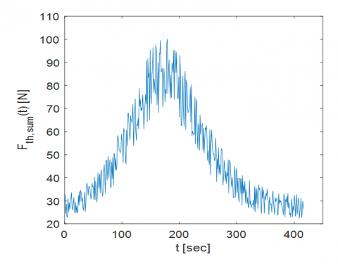
Figure 6. Instantaneous thrust force $F_{\text {th,sum }}(t)$ sampled every second for MODEL1
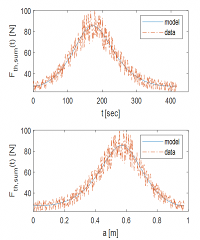
Figure 7. A modelled and sampled instantaneous thrust force $F_{t h, s u m}(t)$ with time $t$ and location $a$ from the fixed enc (chuck) for MODEL1 of the aluminium workpiece sample with length is $l=973 \mathrm{~mm}$ and the diameter is $D=20 \mathrm{~mm}$
The thrust force coefficients from above are $K_{t h}=$ $9.61 \times 10^7 \mathrm{Nm}^{-2}$ and $K_{t h, e}=7.68 \times 10^3 \mathrm{Nm}^{-1}$ for the combination of high-speed steel cutting tool and aluminium workpiece material used. The parameters $w=$ $0.5 \mathrm{~mm}$ and $\Omega=280 \mathrm{rpm}$ were used for the cutting tests. The aluminium workpiece length is $l=973 \mathrm{~mm}$, the diameter is $D=20 \mathrm{~mm}$ and with measured tensile modulus of $E=71.3$ $\mathrm{GPa}$, density $\rho=2832 \mathrm{kgm}^{-3}$ was assumed. The feed is $f=$ $h=0.5 \mathrm{~mm} / \mathrm{rev}$. The feed rate is therefore $v=f \frac{\Omega}{60}=$ $0.0023 \mathrm{~ms}^{-1}$. The thrust force $F_{\text {th,sum }}$ sensed by the dynamometer was sampled every second as shown in Figure 6. It is seen that $F_{t h, s u m}(t)$ minimizes close to the supports where the reactive loading of the tool by the deformed workpiece is minimum. The value of $F_{t h, s u m}(t)$ increased from $15(\mathrm{~N})$ to a maximum value of $100(\mathrm{~N})$ when the time $(\mathrm{t})$ is $200 \mathrm{sec}$ and then starts decreasing to $13(\mathrm{~N})$ when the time $(\mathrm{t})$ is $400 \mathrm{sec}$. This is more obvious in Figure 7 where both the measured and the modelled thrust forces are plotted on the same axes. From Figure 7, it can be seen that $F_{\text {th sum }}(t)$ increased from $15(\mathrm{~N})$ to a maximum value of $80(\mathrm{~N})$ and then starts declining to $13(\mathrm{~N})$ when the time (t) is $400 \mathrm{sec}$. Also, the location at which the instantaneous thrust force maximizes can be clearly read from the graph $(0.6 \mathrm{~m})$. For another sample, the aluminium workpiece length is $l=360 \mathrm{~mm}$ and the diameter is $D=15 \mathrm{~mm}$. The sampled thrust force and the predicted force are shown in Figure 8. This Figure 8 below shows a similar behaviour as the Figures 6 and 7 above for both predicted and experimental values of the cutting force. The graphs show that the developed model was able to capture the behaviour of the workpiece noting that higher cutting forces lower the accuracy of the machining process and the machined part.
Figure 8. A modelled and sampled instantaneous thrust force $F_{t h, s u m}(t)$ with time $t$ and location $a$ from the fixed end (chuck) for MODEL1 of the aluminium workpiece sample with length is $l=360 \mathrm{~mm}$ and the diameter is $D=15 \mathrm{~mm}$.
In general, there is a trade-off between cutting force and MRR. Increasing the material removal rate often requires higher cutting forces, but it can be achieved by optimizing cutting parameters, tooling, and machine setup to strike a balance between these factors. Machinists and engineers use various strategies and calculations to find the optimal combination of parameters for a specific machining operation to maximize MRR while keeping cutting forces within acceptable limits. High cutting forces might result in the workpiece flexing or deforming when machining thin or delicate workpieces. Accuracy issues with the finished part may be caused by this distortion. Using support structures, lowering cutting forces, or choosing other machining techniques are all approaches to reduce workpiece deformation. In machining research and process optimization, estimating cutting force coefficients using experimental techniques and regression models is a typical strategy. There are, however, a number of drawbacks to this approach:
The realization of a set product quality within the restrictions of available resources-equipment, money, and time-can be characterized as the general manufacturing challenge. Unfortunately, it is difficult to guarantee that these requirements will be reached for some product quality parameters, such as flexibility.
In this work, the effects of workpiece flexibility on cutting performance in turning operations was modelled. The model allows the computation of the actual turning productivity. The method involved modelling the static response of the flexible workpiece to the thrust component of cutting forces. The effects of flexibility on the responses of the beam-models on the material removal rate, and the extent of deviation from the intended shape and size were studied. A computational approach verified experimentally was used. The computational approach requires cutting force coefficients, and the coefficients were determined using cutting tests and pseudo inverse regression analysis. The experimental setup for the cutting test is made up of a locally constructed dynamometer for measuring cutting forces, displays on both LCD and computer monitor for taking the readings of the cutting forces, a cutting tool, and a workpiece. The determined force coefficients are highly reliable judging from the coefficients of determination, R2 values of 0.97, 0.89 and 0.93 of the regression calibrating the force coefficients for the tangential, feed, and radial directions which is used to measure the accuracy of the determined force coefficient and it is normally one or close to one as seen here. Effort should be made in future to investigate a case of CNC lathe operations where the workpieces could be modelled as rotating fixed-free (cantilevered) beam due to fixed support at the chuck and unsupported end on the other side of the workpieces as way of improving both accuracy and productivity. The developed computational model can be further worked on to make it simple and versatile for actual industrial application. It is recommended that researchers should improve the machining ability of slender parts through high-performance machining strategies such as cryogenic minimum quantity lubrication (CMQL) machining and Additive Manufacturing by exploration of application of the second order least squares approximated full-discretization method of Song et al. [33], for needed stability analysis and develop comprehensive prediction models that consider the structure deflections of cutting tool/workpiece and the chatter instability simultaneously.
I wish to acknowledge and thank all the authors for their individual contribution to the success of this research. I also want to appreciate the management of The Bells University of Technology for her supports since this research began till date and for providing conducive environment for research and researchers to thrive.
|
Tct |
Complete machine adjusting time, s |
|
Ti |
Controlling or inactive time, s |
|
Tc |
Real machining time, s |
|
TCT |
Time needed for a single changing, s |
|
Tm |
Total time for machining, s |
|
Lc |
Complete cut length, mm |
|
s |
Rate of feed, mm.rev-1 |
|
Ω |
Spindle speed, rpm |
|
$V_c$ |
Speed of cu of cut, m.s-2 |
|
D |
Diameter of job, mm |
|
$T L$ |
Taylor’s Tool Life |
|
Fc |
Tangential cutting force component, N |
|
Nc |
Feed cutting force component, N |
|
Fth |
Thrust cutting force component, N |
|
Fsp |
Shear force component on the shear plane |
|
Nsp |
Normal force component on the shear plane |
|
Frf |
Frictional force component of the rake face |
|
Nrf |
Normal force component of the rake face |
|
rch |
Chip thickness ratio |
|
h |
Undeformed chip thickness (mm) |
|
hch |
Chip thickness, mm |
|
Vch |
Chip velocity on the rake face, m.s-2 |
|
Vt |
Tangential velocity, m.s-2 |
|
w |
Depth of cut, mm |
|
$\sigma_{s p}$ |
Yield normal stress of the material, N.mm-2 |
|
$\tau_{s p}$ |
Yield shear stress of the material, N.mm-2 |
|
Kf |
Feed cutting force coefficient, N.mm-2 |
|
Kt |
Tangential cutting force coefficient, N.mm-2 |
|
Kth |
Thrust cutting force coefficient, N.mm-2 |
|
Kf, e |
Feed edge force coefficient, N.mm-1 |
|
Kt, e |
Tangential edge force coefficient, N.mm-1 |
|
Kth, e |
Thrust edge force coefficient, N.mm-1 |
|
E |
Young’s Modulus, N.mm-2 |
|
I |
Moment of inertia, mm-4 |
|
l |
Length of the workpiece, mm |
|
y |
Beam deflection, mm |
|
F |
The applied load on the beam, N |
|
M1 |
Bending moment at point A, Nm |
|
MAB |
Bending moment at point AB, Nm |
|
MBC |
Bending moment at point BC, Nm |
|
yAB |
Deflection along AB, mm |
|
YBC |
Deflection along BC, mm |
|
R1 |
Reaction at support A, N |
|
R2 |
Reaction at support C, N |
|
$\rho$ |
Density of the workpiece, kg.m-3 |
|
x |
Distance from point A to the point of interest along the length of the workpiece, mm |
|
w(a) |
Actual depth of cut, mm |
|
a |
Distance of the load from fixed end A, mm |
|
b |
Distance of the load from end C, mm |
|
ϑ |
Non-zero approach angle, deg. |
|
w(t) |
Instantaneous depth of cut, mm |
|
MRR |
Material removal rate, kg.m-3 |
|
Dmax |
Maximum diameter of the workpiece, mm |
|
$\bar{D}$ |
Average diameter of the workpiece, mm |
|
m |
Total amount of material removed, kg |
|
t |
Time, s |
|
y(t) |
Instantaneous deflection, mm |
|
yi |
Predicted values |
|
Ti |
Experimental values |
|
R2 |
Coefficient of determination |
|
RMSE |
Root mean square error |
|
MBE |
Mean biased error |
|
MABE |
Mean absolute biased error |
|
MPA |
Mean percentage error |
|
Greek symbols |
|
|
a |
Rake angel, deg. |
|
b |
Friction angle, deg. |
|
$\varphi$ |
Shear angle, deg. |
[1] Yang, Z., Zhu, D., Chen, C., Tian, H., Guo, J., Li, S. (2018). Reliability modelling of CNC machine tools based on the improved maximum likelihood estimation method. Mathematical Problems in Engineering, 2018: Article ID 4260508. https://doi.org/10.1155/2018/4260508
[2] Caggiano, A. (2018). Machining of fibre reinforced plastic composite materials. Materials, 11(3): 442. https://doi.org/10.3390/ma11030442
[3] Kini, M.V., Chincholkar, A.M. (2010). Effect of machining parameters on surface roughness and material removal rate in finish turning of±30 glass fibre reinforced polymer pipes. Materials & Design, 31(7): 3590-3598. https://doi.org/10.1016/j.matdes.2010.01.013
[4] Senesathit, S., Deng, S., Zhang, S., Mohammed, Y., Al Rubaei, A., Yuan, X., Duan, J. (2019). Study and investigate effects of cutting surface in CNC milling process for Aluminum based on Taguchi design method. International Journal of Engineering Research & Technology, 8(12): 288-295. https://doi.org/10.17577/ijertv8is120186
[5] Krishankant, J.T., Bector, M., Kumar, R. (2012). Application of Taguchi method for optimizing turning process by the effects of machining parameters. International Journal of Engineering and Advanced Technology, 2(1): 263-274.
[6] Chen, J.P., Gu, L., He, G.J. (2020). A review on conventional and nonconventional machining of SiC particle-reinforced aluminium matrix composites. Advances in Manufacturing, 8: 279-315. https://doi.org/10.1007/s40436-020-00313-2
[7] Hassan, K., Kumar, A., Garg, M.P. (2012). Experimental investigation of material removal rate in CNC turning using Taguchi method. International Journal of Engineering Research and Applications, 2(2): 1581-1590.
[8] Hacksteiner, M., Duer, F., Ayatollahi, I., Bleicher, F. (2017). Automatic assessment of machine tool energy efficiency and productivity. Procedia CIRP, 62: 317-322. https://doi.org/10.1016/j.procir.2016.06.034
[9] Eberspächer, P., Schraml, P., Schlechtendahl, J., Verl, A., Abele, E. (2014). A model-and signal-based power consumption monitoring concept for energetic optimization of machine tools. Procedia CIRP, 15: 44-49. https://doi.org/10.1016/j.procir.2014.06.020
[10] Hu, S., Liu, F., He, Y., Hu, T. (2012). An on-line approach for energy efficiency monitoring of machine tools. Journal of Cleaner Production, 27: 133-140. https://doi.org/10.1016/j.jclepro.2012.01.013
[11] Abbas, A.T., Abubakr, M., Hassan, M.A., Luqman, M., Soliman, M.S., Hegab, H. (2020). An adaptive design for cost, quality and productivity-oriented sustainable machining of stainless steel 316. Journal of Materials Research and Technology, 9(6): 14568-14581. https://doi.org/10.1016/j.jmrt.2020.10.056
[12] Bagaber, S.A., Yusoff, A.R. (2017). Multi-objective optimization of cutting parameters to minimize power consumption in dry turning of stainless steel 316. Journal of Cleaner Production, 157: 30-46. https://doi.org/10.1016/j.jclepro.2017.03.231
[13] Abbas, A.T., Al-Abduljabbar, A.A., Alnaser, I.A., Aly, M.F., Abdelgaliel, I.H., Elkaseer, A. (2022). A closer look at precision hard turning of AISI4340: Multi-objective optimization for simultaneous low surface roughness and high productivity. Materials, 15(6): 2106. https://doi.org/10.3390/ma15062106
[14] Yan, J., Li, L. (2013). Multi-objective optimization of milling parameters–the trade-offs between energy, production rate and cutting quality. Journal of Cleaner Production, 52: 462-471. https://doi.org/10.1016/j.jclepro.2013.02.030
[15] Chandrasekhar, S., Prasad, N.B.V. (2020). Multi-response optimization of electrochemical machining parameters in the micro-drilling of AA6061-TiB2in situ composites using the Entropy–VIKOR method. Proceedings of the Institution of Mechanical Engineers, Part B: Journal of Engineering Manufacture, 234(10): 1311-1322. https://doi.org/10.1177/0954405420911539
[16] Hegab, H., Darras, B., Kishawy, H. (2018). Towards sustainability assessment of machining processes. Journal of Cleaner Production, 170: 694-703. https://doi.org/10.1016/j.jclepro.2017.09.197
[17] Mallick, A., Dhara, S., Rath, S. (2021). Application of machine learning algorithms for prediction of sinter machine productivity. Machine Learning with Applications, 6: 100186. https://doi.org/10.1016/j.mlwa.2021.100186
[18] Wei, C., Guo, W., Pratomo, E.S., Li, Q., Wang, D., Whitehead, D., Li, L. (2020). High speed, high power density laser-assisted machining of Al-SiC metal matrix composite with significant increase in productivity and surface quality. Journal of Materials Processing Technology, 285: 116784. https://doi.org/10.1016/j.jmatprotec.2020.116784
[19] Niaki, F.A., Haines, E., Dreussi, R., Weyer, G. (2020). Machinability and surface integrity characterization in hard turning of AISI 4320 bearing steel using different CBN inserts. Procedia Manufacturing, 48: 598–605. https://doi.org/10.1016/j.promfg.2020.05.087
[20] Camposeco-Negrete, C., de Dios Calderón-Nájera, J. (2019). Optimization of energy consumption and surface roughness in slot milling of AISI 6061 T6 using the response surface method. The International Journal of Advanced Manufacturing Technology, 103(9–12): 4063-4069. https://doi.org/10.1007/s00170-019-03848-2
[21] Sangwan, K.S., Kant, G. (2017). Optimization of machining parameters for improving energy efficiency using integrated response surface methodology and genetic algorithm approach. Procedia CIRP, 61: 517-522. https://doi.org/10.1016/j.procir.2016.11.162
[22] Pusavec, F., Deshpande, A., Yang, S., M’Saoubi, R., Kopac, J., Dillon, O.W., Jawahir, I. (2015). Sustainable machining of high temperature Nickel alloy–Inconel 718: part 2–chip breakability and optimization. Journal of Cleaner Production, 87: 941–952. https://doi.org/10.1016/j.jclepro.2014.10.085
[23] Khan, A.M., He, N., Li, L., Zhao, W., Jamil, M. (2020). Analysis of productivity and machining efficiency in sustainable machining of titanium alloy. Procedia Manufacturing, 43: 111–118. https://doi.org/10.1016/j.promfg.2020.02.122
[24] Pang, J., Ansari, M., Zaroog, O.S., Ali, M.H., Sapuan, S. (2014). Taguchi design optimization of machining parameters on the CNC end milling process of halloysite nanotube with aluminium reinforced epoxy matrix (HNT/Al/Ep) hybrid composite. HBRC Journal, 10(2): 138-144. https://doi.org/10.1016/j.hbrcj.2013.09.007
[25] Ribeiro, J.E., César, M.B., Lopes, H. (2017). Optimization of machining parameters to improve the surface quality. Procedia Structural Integrity, 5: 355-362. https://doi.org/10.1016/j.prostr.2017.07.182
[26] Qehaja, N., Jakupi, K., Bunjaku, A., Bruçi, M., Osmani, H. (2015). Effect of machining parameters and machining time on surface roughness in dry turning process. Procedia Engineering, 100: 135–140. https://doi.org/10.1016/j.proeng.2015.01.351
[27] Shaw, M.C., Cookson, J.O. (2005). Metal Cutting Principles (Vol. 2, No. 3). New York: Oxford University Press.
[28] Qiu, J. (2018). Modeling of cutting force coefficients in cylindrical turning process based on power measurement. International Journal of Advanced Manufacturing Technology, 99(9-12): 2283-2293. https://doi.org/10.1007/s00170-018-2610-9
[29] Bandapalli, C., Sutaria, B.M., Bhatt, D.V., Singh, K.K. (2017). Experimental investigation and estimation of surface roughness using ANN, GMDH & MRA models in high speed micro end milling of titanium alloy (Grade-5). Materials Today: Proceedings, 4(2): 1019-1028. https://doi.org/10.1016/j.matpr.2017.01.115
[30] Altintas, Y. (2012). Manufacturing Automation (2nd ed.) New York: Cambridge University Press. https://doi.org/10.1017/CBO9780511843723
[31] Cianetti, F., Morettini, G., Palmieri, M., Zucca, G. (2019). Virtual qualification of aircraft parts: test simulation or acceptable evidence? Procedia Structural Integrity, 24: 526-540. https://doi.org/10.1016/j.prostr.2020.02.047
[32] Budynas, R.G., Nisbett, J.K. (2011). Shigle’s Mechanical Engineering Design (Ninth Edition). New York: McGraw-Hill.
[33] Song, C., Peng, Z., Zhao, D., Jin, X. (2023). A whole discretization method for milling stability prediction considering the discrete vibration velocities. Journal of Sound and Vibration, 553: 117687. https://doi.org/10.1016/j.jsv.2023.117687