Inchirah Sari-Ali* | Bachir Chikh-Bled | Omolayo M. Ikumapayi | Zahira Dib | Giulio Lorenzini | Younes Menni
© 2022 IIETA. This article is published by IIETA and is licensed under the CC BY 4.0 license (http://creativecommons.org/licenses/by/4.0/).
OPEN ACCESS
Any alternating electric power supply is always characterized by three reference quantities, which are voltage, electric power and frequency. The generators of power stations are synchronous machines. The present work is based on the modelling of the synchronous machine for a study of the stability of the electricity transmission network. The example considered is a thermal power station of the national network. i.e., Algiers port power station. We have developed a computer program based on MATLAB to simulate the calculations of our multi-variable system. The study presented in this article examines the static stability of a thermal power plant. To make this study a reality, it is necessary to model the synchronous machine. We present the three models of the synchronous machine by emphasizing the role of the shock absorbers and the smoothness of the model with three windings. This work is supported by a spectral analysis based on the eigenvalues of the system.
modelling, synchronous machine, static stability, shock absorbers, electrical network
Electric energy is a key element of daily life in our civilization. All over the world, electricity has found many applications, in various fields of life, in industry, agriculture, transport and household uses. Synchronous machines occupy an important place in industrial equipment. They now represent an important part of the market for electromechanical energy converters and cover a very wide power range. They are widely used as a reciprocating or high power electric motor [1]. Most of the energy available in power grids comes from thermal and hydroelectric power stations. They use synchronous generators to convert mechanical energy from a turbine into electrical energy. Thermal power plants use turbo-generators driven by steam turbines, while hydro-generators in hydraulic plants are driven by the force of water.
The modeling of synchronous generators has been the subject of several research studies for several decades. With the development of computer science, work on their modeling has increased with a view to their simulation in dynamic operation. This requires precise knowledge, for each operating point, of the electrical, magnetic and mechanical parameters [2]. The calculation of the dynamic behavior of synchronous machines is currently done almost exclusively on the basis of Park's two axis theory [3]. The model of the synchronous machine is based on the laws of electrical circuits, known as Kirchhoff's laws. This type of model is often used for the description of the behavior of the machine during transient operation and in machine control. In spite of the simplification carried out by the transformation of Park, the study and the analysis of the synchronous machine remain rather difficult. To this end, the representation of the electromagnetic coupling of the two axes d and q by equivalent diagrams of inductors and resistances is of great interest for the analysis of the operation of the machine [4-6] and for the identification parameters [7, 8]. Important studies have been done recently in the scope of improving stability in different modalities [9-20] as shown in Table 1.
In our work, we are interested in mathematical modeling and techniques for offline identification of parameters of wound rotor synchronous machines with and without dampers and the simulation of their operation. The phenomenon of synchronous machine stability has received great attention in the past and will receive increasing attention in the future.
This phenomenon is aimed at the operation and planning of the electricity network. There are two types of stability, stability with respect to small disturbances and transient in the opposite case [21]. The example treated is that of the "Algiers-port" power plant of the national network.
The synchronous machine consists of a moving part: the rotor and a fixed part: the stator. The two parts are made up of two main elements. One is called ferromagnetic and it is used to conduct the magnetic flux and withstand the forces, while the other is called a winding and is made of copper or aluminum conductors. These conductors form a coil. All of the coils are magnetically coupled.
In motor operation, the stator windings are supplied by a three-phase pulsating voltage system w=p.Ω. They then create a rotating field at the Ω pulsation. The field created by the inductor, fixed with respect to the rotor (driven by a rotational speed Ω) rotates in synchronism with the field created by the armature. These two fields interact. The torque thus created drives the machine at speed w.
Table 1. The synchronous machine's modeling
|
Author (s) |
Contribution |
|
Weiss et al. [9] |
For networks with synchronous generators, a stability theorem has been developed. |
|
Sekizaki et al. [10] |
A single-phase synchronous inverter was developed and integrated into a single-phase microgrid to improve frequency stability. |
|
Eltamaly et al. [11] |
For optimal voltage regulation, use adaptive static synchronous compensation techniques with the transmission system. |
|
Dahiya [12] |
Stability increase of the doubly fed induction generator integrated system using a superconducting magnetic energy storage connected static compensator. |
|
Shivratri et al. [13] |
Machines with a fast current loop that are virtual synchronous. |
|
Masood et al. [14] |
Strengthening of the system in the presence of strong winds. |
|
Grdenić et al. [15] |
Assessment of the impact of AC network modeling on AC systems with VSC HVDC converters' small-signal stability. |
|
Dashti et al. [16] |
In electrical energy distribution networks, a study of fault prediction and localisation methods is presented. |
|
Shahriar et al. [17] |
Low-frequency oscillations in electric networks can be dampened in real time using a neurogenetic technique. |
|
Ghasemi-Marzbali [18] |
A coordinated technique for the stability of multi-machine power systems. |
|
Villa-Acevedo et al. [19] |
The use of a kernel extreme learning machine approach to monitor long-term voltage stability in power system areas. |
|
Øyvang et al. [20] |
For transient power system research, models of synchronous generators with excitation systems. |
3.1 Synchronous machine modeling
The synchronous machine is an alternating current machine in which the frequency of the induced voltage generated and the speed are in a constant ratio [22].
The model that we distinguish is based on the following simplifying assumptions [2]:
·Spatial distribution of sinusoidal magnetomotive forces.
·Magnetic circuit is unsaturated.
·Notch effects are neglected.
·Negligible ferromagnetic losses.
·The influence of temperature on the characteristics is not taken into account.
Modeling is an important step in the analysis and design of systems. With these assumptions, the different electrical circuits satisfy the following fundamental electrical equation:
According to the generalized Ohm law, the voltage of a circuit with resistance R crossed by a flow $\phi$ is written:
$U_i=R I+\frac{d \phi}{d t}$ (1)
In a machine the voltage equation for winding J is written [22]:
$U_j=R_j I_j+\frac{d \phi_j}{d t}=R_j I_j+\frac{d}{d t} \Sigma \phi_{j p}$ (2)
The system of voltage equations of the synchronous machine obtained by applying relation (1) to the different circuits is given by (3) [23]:
Stator equations in phase quantities:
$U_a=R_s I_b+\frac{d \phi_a}{d t}$
$U_b=R_s I_b+\frac{d \phi_b}{d t}$
$U_c=R_s I_c+\frac{d \phi_c}{d t}$ (3)
Equations of rotor voltages in phase quantities:
$U_f=R_f I_f+\frac{d \phi_f}{d t}$
$0=R_d I_d+\frac{d \phi_d}{d t}$
$0=R_q I_q+\frac{d \phi_q}{d t}$ (4)
with, Uabc is the instantaneous voltages of stator phases a, b and c, Uf the DC rotor excitation voltage, Iabc the instantaneous currents of stator phases a, b and c, If the rotor excitation current, $\phi_{a b c}$ the total fluxes through the stator phases a, b, and c, $\phi_f$ the flux through the rotor circuit, RS the is the resistance per stator phase and, Rf is the rotor resistance (inductor).
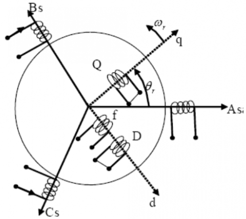
3.2 Schematical representation of the machine
It is given as shown in Figure 1, with:
A, B, C: stator windings.
F: inductor winding.
D: damper winding along the direct axis.
Q: damper winding along the quadratic axis.
d: stator winding along the direct axis.
q: stator winding along the quadratic axis.
Figure 1. Synchronous machine: PARK model [24]
3.3 Park transformation
To simplify the calculations, a change of variable called transformation of PARK is carried out. This transformation consists in replacing the fixed stator windings (a, b, c) by two fictitious windings (d, q) integral with the rotor. For all three vectors of currents, voltages and stator flux, we obtain [25]:
$\left[U_s\right]=[P(\theta)]\left[U_P\right]$
$\left[I_s\right]=[P(\theta)]\left[I_P\right]$
$\left[\phi_s\right]=\left[P(\theta)\left[\phi_P\right]\right.$ (5)
with the matrix [P (θ)] which is given by the following expression [25]:
$[P(\theta)]=\sqrt{\frac{2}{3}}\left[\begin{array}{ccc}\cos \theta & \cos \left(\theta-\frac{2 \pi}{3}\right) & \cos \left(\theta-\frac{2 \pi}{3}\right) \\ \sin \theta & \sin \left(\theta-\frac{2 \pi}{3}\right) & \sin \left(\theta-\frac{2 \pi}{3}\right) \\ \frac{1}{\sqrt{2}} & \frac{1}{\sqrt{2}} & \frac{1}{\sqrt{2}}\end{array}\right]$ (6)
[P(θ)]: Standardized matrix which preserves the power. By substituting Eq. (4) in Eq. (3), we obtain for the stator the following equations:
$U_d=-\frac{d \phi_d}{d t}-\phi_q \frac{d \theta}{d t}-R_s I_d$
$U_q=-\frac{d \phi_q}{d t}+\phi_d \frac{d \theta}{d t}-R_s I_q$
$U_0=-\frac{d \phi_0}{d t}-R_s I_0$ (7)
where, $\phi_d:$ the total flux through the coil equivalent to the stator placed on the direct axis d. $\phi_q:$ the total flux through the coil equivalent to stator placed in quadratic q. $\phi_0:$ the total flux relating to the homopolar component.
Assuming that the assembly is in star coupling, the zero sequence component $V_0\left(I_0, \phi_0\right)$ confused with the neutral, the system of equation becomes:
$U_d=-\frac{d \phi_d}{d t}-\phi_q \frac{d \theta}{d t}$
$U_q=-\frac{d \phi_q}{d t}+\phi_d \frac{d \theta}{d t}$ (8)
Such that Ud, Uq are voltages along the direct axis and in quadrature. These two equations must be completed by the following equations:
a) The excitation voltage
$U_f=\frac{d \phi_f}{d t}+R_f I_f$ (9)
b) The tensions of the dampers following the direct axis and in quadrature are given by the following expressions:
$0=\frac{d \phi_d}{d t}-R_d I_d$
$0=\frac{d \phi_q}{d t}-R_q I_q$ (10)
3.4 Mechanical equation
The movement of the rotor is given by the equation of the rotating masses:
$C=w R^2 \alpha / g=\frac{J d w}{d t}$ (11)
where, C is the acceleration torque acting on the rotor, J=wR2 the moment of inertia of the rotating masses, g the acceleration of gravity, and α is the angular acceleration.
The equation of the difference between the rotor and the synchronous reference is given by:
$\delta=w_s t+w_m$ (12)
The equation of rotating masses becomes:
$J d w / d t=C_m-C_e$ (13)
Cm and Ce are respectively the mechanical torque of the machine and the resistive electrical torque transmitted to the armature of the machine. The latter is given by:
$C_e=\frac{3}{2}\left(\phi_d i_d-\phi_q i_q\right)$ (14)
4.1 Non-linear system of the three models of the machine
Electrical and mechanical equations:
4.1.1 Single winding model
$\frac{d E^{\prime}}{d t}=\frac{1}{T_{d_0}^{\prime}}\left[e f d-E_q^{\prime}-\left(x_d-x_d^{\prime}\right) i_d\right]$
$\frac{d \omega}{d t}=\frac{1}{T_a}\left(P_m-P_e\right)$
$\frac{d \delta}{d t}=\omega_0(\omega-1)$ (15)
4.1.2 Two winding model
$\begin{aligned} \frac{d E^{\prime}}{d t} & =\frac{1}{T_{d_0}^{\prime}}\left[e f d-E_q^{\prime}-\left(x_d-x_d^{\prime}\right) i_d\right] \\ \frac{d \omega}{d t} & =\frac{1}{T_a}\left(P_m-P_e\right) \\ \frac{d \delta}{d t} & =\omega_0(\omega-1)\end{aligned}$ (16)
4.1.3 Three winding model
$\frac{d E_q^{\prime}}{d t}=\frac{x_d^{\prime \prime}-x_a}{x_d^{\prime}-x_a} \frac{1}{T_{d_0}^{\prime}}(e f d-e i f)$
$\frac{d E_q^{\prime \prime}}{d t}=\frac{d E_q^{\prime}}{d t}+\frac{d E_Q^{\prime}}{d t}$
$\frac{d E_d^{\prime \prime}}{d t}=\frac{1}{T_{q_0}^{\prime \prime}} E i_Q$
$\frac{d \omega}{d t}=\frac{1}{T_a}\left(P_m-P_e\right)$
$\frac{d \delta}{d t}=\omega_0(\omega-1)$ (17)
4.2 Linear system of infinite machine-network models
The linearization of the infinite machine-network model around an operating point X0=[Pe, Qe, ω, Vr] leads us to a linear system given by the formula [26-28]:
$\dot{X}=a x+b u$
$Y=c x+d u$ (18)
with, x is the groups the state variables, u the regroup the command variables, Y the groups the output variables, a and b represent the linearization coefficients.
4.2.1 Model with one winding
Represents the model of the machine without damper winding [23]:
$\dot{\Delta E_q^{\prime}}=\frac{1}{T_{d_0}^{\prime}} \Delta e f d-\frac{1}{K_3 T_{d_0}^{\prime}} \Delta E_q^{\prime}-\frac{K_4}{T_{d_0}^{\prime}} \dot{\Delta \delta}$
$\dot{\Delta \omega}=\frac{1}{T_a}\left(\Delta P_m-\Delta P_e\right)$
$\dot{\Delta \delta}=\omega_0 \Delta \omega$ (19)
4.2.2 Model with two windings
Represents the model of the machine with a damping winding [23]:
$\dot{\Delta E_q^{\prime}}=\frac{1}{T_{d_0}^{\prime}} \Delta e f d-\frac{1}{K_3 T_{d_0}^{\prime}} \Delta E_q^{\prime}-\frac{K_4}{T_{d_0}^{\prime}} \dot{\Delta \delta}$
$\dot{\Delta E_d^{\prime \prime}}=-\frac{1}{T_{q_0}^{\prime \prime}} R_4 \Delta E_d^{\prime \prime}-\frac{K_5}{T_{q_0}^{\prime \prime}} \dot{\Delta \delta}$
$\dot{\Delta \omega}=\frac{1}{T_a}\left(\Delta P_m-\Delta P_e\right)$
$\dot{\Delta \delta}=\omega_0 \Delta \omega$ (20)
4.2.3 Three winding model
It shows the machine model with 2 damping windings [23]:
$\dot{\Delta E}_q^{\prime}=\frac{1}{T_{d_0}^{\prime}}\left[S_1 \Delta e f d-S_2 \Delta E_q^{\prime}+S_3 \Delta E_q^{\prime \prime}+S_4 \Delta E_d^{\prime \prime}+S_5 \dot{\Delta \delta}\right]$
$\dot{\Delta E}_d^{\prime \prime}=\frac{S_1}{T_{d_0}^{{\prime}}} \Delta {efd}-\left(\frac{S_2}{T_{d_0}^{\prime}}+\frac{S_8}{T_{d_0}^{\prime \prime}}\right) {\Delta E}_q^{\prime}+\left(\frac{S_4}{T_{d_0}^{\prime}}+\frac{S_9}{T_{d_0}^{\prime \prime}}\right)+\left(\frac{S_3}{T_{d_0}^{\prime}}-\frac{1}{T_{d_0}^{\prime \prime}}\right) \Delta E_q^{\prime \prime}+\left(\frac{S_5}{T_{d_0}^{\prime}}+\frac{S_{10}}{T_{d_0}^{\prime \prime}}\right) \Delta \delta$
$\dot{\Delta E}_d^{\prime \prime}=\frac{1}{T_{q_0}^{\prime \prime}}\left(\Delta E_d^{\prime \prime}+S_6 \Delta \delta-S_7 \Delta E_q^{\prime \prime}\right)$
$\dot{\Delta} \omega=\frac{1}{T_a}\left(\Delta P_m-\Delta P_e\right)$
$\dot{{\Delta} \delta}=\omega_0 \Delta \omega$ (21)
For the simulation of the linear model of the synchronous machine connected to an infinite network, we consider the constant inputs equal to their nominal values, and we based ourselves on the use of the MATLAB which facilitates the simulation calculations of our multivariate system.
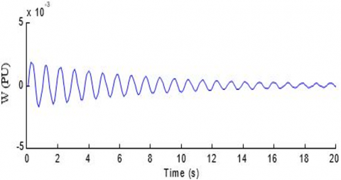
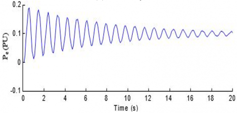
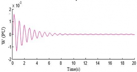
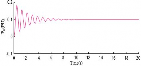
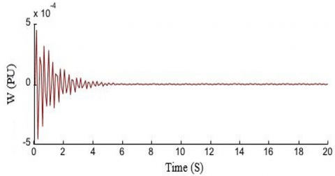
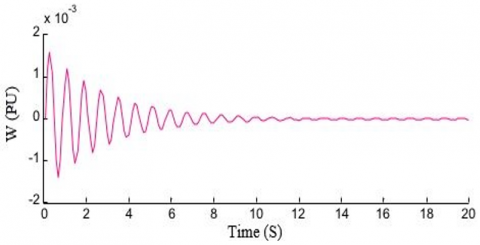
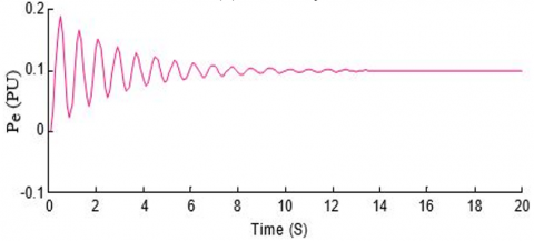
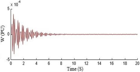
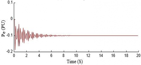
From the initial conditions [y, x]=Lsim (A, B, C, u, x, T) provides the outputs and states of the system in the form of a matrix. We simulated the three models of the synchronous machine connected to an infinite network. For a nominal speed, the results are given by the Figures 2-4. The curves shown in Figures 2-7 represent the simulation results of the synchronous machine connected to the infinite network.
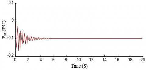
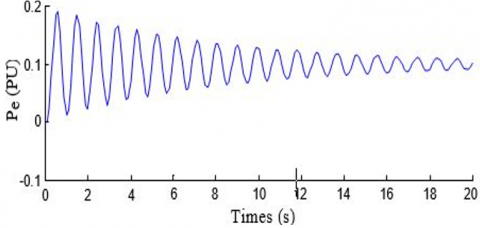
For two types of tests, i.e. nominal speed; sudden increase in load (Xe=0.7P.u). Note that for a given speed and electric power, the three-winding model is thinner compared to the other two models for the two tests. However, the dynamic responses of the system evolve as follows:
·For the three-winding model, the electrical quantities stabilize after a period of 5 seconds at nominal speed and after 8 seconds for the sudden increase in load.
·For the two-winding model, the electrical quantities stabilize after a period of 10 seconds at nominal speed and after 12 seconds for the sudden increase in load.
·The electrical quantities of the single winding model oscillate with low damping for both types of tests.
A physical process must have certain performances with respect to a disturbance, one can quote the stability of the system making it possible to avoid the influence of these disturbances on its operation. Our study is based on the static stability of the electrical network which is necessary for low disturbances (imbalance between production and consumption).
(a) Velocity
(b) Electric power
Figure 2. Simulation of the first type [Single winding model] for nominal operation
(a) Velocity
(b) Electric power
Figure 3. Simulation of the second type [Two-winding model] for nominal operation
(a) Velocity
(b) Electric power
Figure 4. Simulation of the third type [three winding model] for nominal operation
(a) Velocity
(b) Electric power
Figure 5. Simulation of the first type [Single winding model] for a disturbance Xe=0.7 Pu
(a) Velocity
(b) Electric power
Figure 6. Simulation of the second type [two-winding model] for a disturbance Xe=0.7 Pu
(a) Velocity
(b) Electric power
Figure 7. Simulation of the third type [three-winding model] for a disturbance Xe=0.7 Pu
There are two types of stabilities:
· External stability: the necessary and sufficient condition for this type of stability is given by the following expression [21]:
$\int_0^{\infty}|h(t)| d t<M<\infty \quad M \in R$ (22)
The system is in external stability if all the poles of the transfer function are located in the left half plane.
· Internal stability (exponential stability):
The realization of the linear or exponential system is stable if the solution x (t) is of the following form [21, 22]:
$x(t)=A x(t) \quad x\left(t_0\right)=x_0 \quad t \geq t_0$
$x(t) \rightarrow 0$
$t \rightarrow \infty$ (23)
$R_e\left(\lambda_i(A)\right)<0 \Rightarrow \int_0^{\infty}|h(t)| d t<M<\infty$ (24)
So the realization is stable if and only if Re (λi (A)) < 0 such that λi (A) are eigenvalues of the matrix A.
This part includes the study of static stability by a spectral analysis based on the real part of the eigenvalues. The computation of the eigenvalues of the matrix A provides a direct criterion of static stability.
The real part of an eigenvalue measures the damping of the corresponding model. If the imaginary part exists, it represents the image of the oscillation frequency of the associated eigen model.
To analyze the static stability, a perturbation is carried out on the parameters Xe, Pe, Qe for the three models.
After execution of the program, the results obtained are grouped together in the following Table 2.
Table 2. Analysis of the eigenvalues of the matrix A for the three models
|
Own values |
Xe |
Pe |
Qe |
Results |
Models |
||
|
0.56 -0.47 +2.10 j -0.47 -2.10 j |
1.5 |
1.5 |
-0.75 |
Unstable System |
One Winding |
||
|
-0.0049 -0.62 +10j -0.62 -10j |
0.01 |
Stable System |
|||||
|
-11.74 2.14 -24577 -15.90 |
1.2 |
1.2 |
-1.5 |
Unstable System |
Two Windings |
||
|
-16.54 -0.20 +3.11j -0.20 -3.11j -23.55 |
0.55 |
Stable System |
|||||
|
0.32 +54.74j 0.32 -54.74j -16.41 -1.23 -5.38 |
1.5 |
1.5 |
-1.75 |
Unstable System |
Three Windings |
||
|
-0.66 +24.23j -0.66 -24.23j -15.07 -1.13 -5.43 |
0.55 |
Stable System |
|||||
The decrease in line reactance after disturbance is of considerable help in maintaining the static stability of the network.
For the simulated disturbance, the modes of the spectrum show that the system is unstable, this case corresponds to limit operating regimes where the real part of the roots passes through zero.
To this end, the line impedance has been reduced, which is a factor influencing the stability of the system.
This reduction makes it possible to:
Make the real part of the eigenvalues negative, Xe=0.01 for the one winding model, Xe=0.55 for the two winding model, Xe=0.55 for the three winding model.
Stabilizes the quantities (speed, electric power) at their nominal values.
We have shown the validity of damping windings on the behavior of a synchronous machine connected to a powerful network through a power transmission line.
To this end, our study requires the modeling of the three models of the synchronous machine. The approach adopted consists in linearizing all the equations around an operating point.
The study of static stability is developed by a spectral analysis based on the eigenvalues of the system, concluding that the network voltage and the line reactance play a primary role in the stability of the operating regime.
The results obtained by the three models made it possible to show the smoothness of the model with three windings.
[1] Badraoui, M., Bereksi Reguig, M. (2016). Etude et modélisation du moteur synchrone simple et double étoile avec application de la commande backstepping à la machine synchrone. Mémoire de Master, Université de Tlemcen.
[2] Radjeai, H. (2018). Contribution à l'amélioration des modèles mathématiques des machines synchrones. Doctoral dissertation.
[3] Park, R.H. (1929). Two-reaction theory of synchronous machines generalized method of analysis-part I. Transactions of the American Institute of Electrical Engineers, 48(3): 716-727. https://doi.org/10.1109/T-AIEE.1929.5055275
[4] Niewierowicz, T., Escarela-Perez, R., Campero-Littlewood, E. (2005). Frequency-dependent equivalent circuit for the representation of synchronous machines. IEE Proceedings-Electric Power Applications, 152(3): 723-730. https://doi.org/10.1049/ip-epa:20045214
[5] Slemon, G.R., Awad, M.L. (1999). On equivalent circuit modeling for synchronous machines. IEEE Transactions on Energy Conversion, 14(4): 982-988. https://doi.org/10.1109/60.815017
[6] Wamkeue, R., Kamwa, I., Dai-Do, X. (1999). Short-circuit test based maximum likelihood estimation of stability model of large generators. IEEE Transactions on Energy Conversion, 14(2): 167-174. https://doi.org/10.1109/60.766977
[7] Jin, Y., El-Serafi, A.M. (1990). A'three transfer functions' approach for the standstill frequency response test of synchronous machines. IEEE Transactions on Energy Conversion, 5(4): 740-749. https://doi.org/10.1109/60.63148
[8] Kamwa, I., Viarouge, P., Dickinson, E.J. (1991). Identification of generalized models of synchronous machines from time-domain tests. In IEE Proceedings C-Generation, Transmission and Distribution, 138(6): 485-498. https://doi.org/10.1049/ip-c.1991.0063
[9] Weiss, G., Dörfler, F., Levron, Y. (2019). A stability theorem for networks containing synchronous generators. Systems & Control Letters, 134: 104561. https://doi.org/10.1016/j.sysconle.2019.104561
[10] Sekizaki, S., Matsuo, K., Sasaki, Y., et al. (2018). A Development of single-phase synchronous inverter and integration to single-phase microgrid effective for frequency stability enhancement. IFAC-PapersOnLine, 51(28): 245-250. https://doi.org/10.1016/j.ifacol.2018.11.709
[11] Eltamaly, A.M., Mohamed, Y.S., El-Sayed, A.H.M., Elghaffar, A.N.A. (2020). Adaptive static synchronous compensation techniques with the transmission system for optimum voltage control. Ain Shams Engineering Journal, 11(1): 35-44. https://doi.org/10.1016/j.asej.2019.06.002
[12] Dahiya, A.K. (2021). Superconducting magnetic energy storage coupled static compensator for stability enhancement of the doubly fed induction generator integrated system. Journal of Energy Storage, 44: 103232. https://doi.org/10.1016/j.est.2021.103232
[13] Shivratri, S., Kustanovich, Z., Weiss, G., Shani, B. (2020). Virtual synchronous machines with fast current loop. IFAC-PapersOnLine, 53(2): 12422-12428.
[14] Masood, N.A., Mahmud, S.U., Ansary, M.N., Deeba, S.R. (2022). Improvement of system strength under high wind penetration: A techno-economic assessment using synchronous condenser and SVC. Energy, 123426. https://doi.org/10.1016/j.energy.2022.123426
[15] Grdenić, G., Delimar, M., Beerten, J. (2020). Assessment of AC network modeling impact on small-signal stability of AC systems with VSC HVDC converters. International Journal of Electrical Power & Energy Systems, 119: 105897. https://doi.org/10.1016/j.ijepes.2020.105897
[16] Dashti, R., Daisy, M., Mirshekali, H., Shaker, H.R., Aliabadi, M.H. (2021). A survey of fault prediction and location methods in electrical energy distribution networks. Measurement, 184: 109947. https://doi.org/10.1016/j.measurement.2021.109947
[17] Shahriar, M.S., Shafiullah, M., Rana, M.J., Ali, A., Ahmed, A., Rahman, S.M. (2020). Neurogenetic approach for real-time damping of low-frequency oscillations in electric networks. Computers & Electrical Engineering, 83: 106600. https://doi.org/10.1016/j.compeleceng.2020.106600
[18] Ghasemi-Marzbali, A., Ahmadiahangar, R. (2021). A coordinated strategy for multi-machine power system stability. Applied Soft Computing, 110: 107742. https://doi.org/10.1016/j.asoc.2021.107742
[19] Villa-Acevedo, W.M., López-Lezama, J.M., Colomé, D.G., Cepeda, J. (2022). Long-term voltage stability monitoring of power system areas using a kernel extreme learning machine approach. Alexandria Engineering Journal, 61(2): 1353-1367. https://doi.org/10.1016/j.aej.2021.06.013
[20] Øyvang, T., Hegglid, G.J., Lie, B. (2018). Models of synchronous generators with excitation system, for transient power system studies. IFAC-PapersOnLine, 51(2): 91-96. https://doi.org/10.1016/j.ifacol.2018.03.016
[21] Pierre, M. (2006). Electrotechnique. Aide mémoire Paris.
[22] Anderson, P.M., Fouad, A.A. (1977). Power system control and stability. Press AMES, IOWA, USA.
[23] Sari-Ali, I., Bouayed, N. (2000). Modélisation de la machine synchrone vis à vis d’une stabilité statique d’un réseau électrique. Mémoire de DES, Université de Tlemcen.
[24] Mrabent, Z. (1996). Etude et analyse de la robustesse du régulateur de tension vis à vis d’une stabilité statique: cas de la centrale d’Alger port. Thèse de Magister, Université de Tlemcen.
[25] Ellouch, M., Hadj, Abdellah, H., Dhifoui, R. (1996). Régimes dynamiques de la machine synchrone connectée à un réseau puissant. Thèse de Magister, Université de Tlemcen.
[26] Ghomri, L. (1996). Analyse et synthèse de régulation robuste vis-à-vis de la stabilité transitoire, Thèse de Magister, Université de Tlemcen.
[27] Demello, F.P., Concordia, C. (1969). Concepts of synchronous machine stability as affected by excitation control. IEEE Transactions on Power Apparatus and Systems, 88(4): 316-329.
[28] Kalil, H.K. (1992). Non linear systems. Michigan State University.