Vo Thanh Ha
© 2022 IIETA. This article is published by IIETA and is licensed under the CC BY 4.0 license (http://creativecommons.org/licenses/by/4.0/).
OPEN ACCESS
This paper describes the design and the simulation of a non-linear controller for a two-mass system (TMS) based on the backstepping-sliding mode control combined with a load torque neural network observer. The aim is to control the actual angular speed matching with the angular reference speed. The backstepping-sliding mode controller is designed based on the Lyapunov standard. The proposed neural network can torque estimate to approximate an appropriate value for unknown factors even when it is affected by the bounded disturbance.
backstepping, sliding mode control, neural network, two-mass system, FOC, NN-observer, TMS
In most of the electrical servo, robot arms drive, wind turbine systems, and paper manufacturing, roll mill drive have a two-mass drive structure flexible. In this TMS the main problem to be considered is the resonance oscillation at the shaft between motor and load. Thus, it can be led to loss of stability for the drive system in case of the motor operation at low and unsatisfactory speed and torque response [1, 2]. Therefore, it is necessary to have a control method or mechanical solution to reduce or supper the resonance oscillation. Currently, there are some different control methods to speed control for TMS such as PID, PI-D, sliding mode, flatness based, backstepping, fuzzy. In the conventional control [3], PID controller is common applied in the industrial, because of its simplicity and less dependent on the drive parameter. This PID control method is to design a transfer function balanced with standard function to calculate control coefficients such as Kp, Ki, KD. However, the two-mass system is a nonlinear drive system, so this PID controller for high efficiency when is not affected by noise. In the other study [4], the m-IPD speed controller gains for TMS with Kp, Ki, KD, and TD coefficients are determined by calculating and choosing the appropriate coefficients for m-IPD speed controller, thus, the drive system responds to the desired load speed. This controller for positive results gives better than PID controller, however unresolved problem resonance oscillation at coupling axis. In addition, follow [5-7] presented the flatness-based control is employed to solve the flux and speed control problem of the system. The system can operate at field weakening region. The simulation results show that high dynamic and suppression of the mechanical oscillation of the drive system can be achieved. And follow [8, 9], backstepping control is used to control the flux and speed of the system. The simulation results show that the drive's mechanical oscillation has been suppressed, however, response speed delays when there is a change in engine parameters. In addition, this paper [10] had given a design method of vibration suppression controller for 3 mass resonance system using a fuzzy controller for speed load. This controller is reduced resonance oscillation in the shaft. However, the controller has not been studied and evaluated for its robustness when the drive system is affected by interference. In the other study [11], slide mode control (SMC) is an efficient simple method of nonlinear control. However, this controller needs to know the parameters of the object model as well as the upper limits of the components on the uncertainty of the model. SMC takes the form of a sgn (.) function and there is a chattering of states around the slip surface 0. In addition, the design of controls for TMS often assumes that all the state variables that are feedback back to the controller are taken by the sensors [12].
To simplify the control structure and increase the performance of the control system, thus estimation of state variables of the two-mas system such as moving horizon estimation (MHE), Luenberger, Kalman filter, and Neural network are actively studied. The main reason is that the state variable is difficult to determine accurately during the operation of this drive system. Chaitanya et al. [12] presents the issues of applying tools to estimate the horizon moving to reconstruct the state variables in improving the control structure of a two-mass system of MHE. Additionally, Shahgholian et al. [13] required dynamic states are recognized based on the error between the reference and estimator outputs, the additional differences between electromagnetic and shaft torque, and its derivatives by a modified fuzzy Luenberger Observer. Depending on these signals, fuzzy systems determine the location of the observer poles [14]. Moreover, the advantages of the Kaman filter with time-varying parameters can be regarded as system noise and can be taken into account for the design. Hence, this filter can be more powerful in principle for parameters identification than Luenberger observers. Moreover, they seem well suited when physical parameters and states have to be estimated simultaneously, which requires an adaptation of feedback gain [15]. Currently, the ability of neural networks (NNs) in controlling nonlinear systems has been studied by Holten et al. [16, 17]. In fact, the adaptation operation of neural networks makes them powerful tools to observe system states without any a priori knowledge about the system dynamics. This paper presented estimates the load moment by radial basis function neural network observer (RBF-NN). In the paper [18-22] nonlinear-in-parameters neural network is employed in flexible joint manipulators. The observer exhibits its advantages in dealing with highly nonlinear system without prior knowledge on system dynamics. In the paper, the load moment is estimated by radial basis function neural network observer (RBFNN). This state variable is difficult to determine accurately during the operation of this drive system.
The content of the paper will be presented as follow sections. First, the model of a two-mass system, then the speed control loop is designed by backstepping-sliding mode control, and the load torque observer is done by RBFNN. Next, the efficiency of the control method is proven by MATLAB/Simulation. Finally, some conclusions and perspectives are presented.
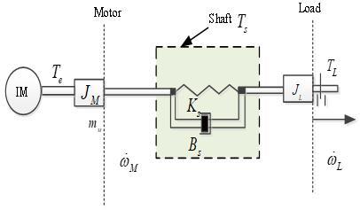
Typical configuration of a TMS shows as Figure 1 and Figure 2 [12]:
Figure 1. Structure of a two-mass system
Figure 2. Structure of the mathematical model of a TMS
The system can be described by the following linear dynamical Eq. (1). It is state model of motor speed, and load. In addition, it is state model of shaft torque.
$\dot{\omega}_M=\frac{1}{J_M}\left(T_e-T_s\right)$
$\dot{\omega}_L=\frac{1}{J_L}\left(T_s-T_L\right)$
$\dot{T}_s=K_s\left(\omega_M-\omega_L\right)$ (1)
where: $\dot{\omega}_M, \dot{\omega}_L$ are motor speed, load speed; $T_e ; T_L ; T_s$ are motor, load and shaft torque; $B_s$ is shaft damping coefficient; $K_s$ is shaft stiffness.; $J_L$ is inertia load torque; State variables are $\dot{\omega}_M, \dot{\omega}_L$; Control variables are $\omega_L, T_L$.
The design of the backstepping-sliding mode control and load torque RBFNN observer can be summarized as following:
Step 1: Determining reference shaft torque
Based on Lyapunov standard with V function is shown:
$V_1=\frac{1}{2} e_L^2$ (2)
$e_L=\omega_L-\omega_{L d}$ (3)
where, $\omega_L ; \omega_{L d}$ are actual and reference angular load speed.
The derivative of candidate Lyapunov function can be defined as following Eq. (4):
$\dot{V}_1=e_L \dot{e}_L=e_L\left(\dot{\omega}_L-\dot{\omega}_{L d}\right)=e_L\left(\frac{1}{J_L}\left(T_s-T_L\right)-\dot{\omega}_{L d}\right)$ (4)
From Eq. (4), taking as the virtual control, it is suggested that the reference shaft torque is designed as:
$T_{s d}=\hat{T}_L-J_L\left(-\dot{\omega}_{L d}+c_l e_L\right)$ (5)
where, $\hat{T}_L$ is load torque estimation which $c_1$ is provided by the RBF neural network; is a positive coefficient.
Step 2: Determining reference load angular
Since the load speed model (1), the shaft torque is defined by Eq. (6):
$T_s=e_{T s}+T_{s d}$ (6)
where, $e_{T s}$ is tracking errors for actual and reference shaft torque.
The derivative of candidate Lyapunov function can be defined as following Eq. (7):
$\begin{aligned} \dot{V}_1 &=e_L\left(\frac{1}{J_L}\left(e_{T s}+T_{s d}-T_L\right)-\dot{\omega}_{L d}\right)=-c_1 e_L^2+\frac{1}{J_L} e_L e_{T s}+\frac{1}{J_L} e_L\left(\hat{T}_L-T_L\right) \end{aligned}$ (7)
Next the derivative of candidate Lyapunov function with tracking errors for shaft torque can be shown by Eq. (8):
$\begin{aligned} \dot{V}_2=\dot{V}_L+e_{T s} \dot{e}_{T s}=-c_1 e_L^2+e_{T s} \left(\frac{1}{J_L} e_L+K_s\left(\omega_M-\omega_L\right)-\dot{T}_{s d}\right)+\frac{1}{J_L} e_L\left(\hat{T}_L-T_L\right) \end{aligned}$ (8)
where, $W^T$ is weight value of RBF, $\hat{W}^T$ denotes weight value estimation; h is radial-basis function vector in the hidden layer of RBF; $\mathcal{E}$ is an error.
Gaussian function value for neural net i in hidden layer is shown as:
$h_i=\exp \left(\frac{\left\|W_L-c_i\right\|}{b^2}\right)$ (9)
where, $c_i$ denotes value of center point of the Gaussian function of neural net i for the $i_{t h}$ input, $b_i$ represent the width value of Gaussian function for neural net i. The hidden layer has one layer in the neural word. The role of the hidden layer is estimable denotes weight value by Gaussian function to find torque estimate suite for this two-mass system.
In this case, assuming that $\mathcal{E}$ is ignored leading to $\tilde{W}=\hat{W}-W$. Eq. (8) can be rewritten as follow:
$\begin{aligned} \dot{V}_2=&-e_L^2+e_{T s}\left(\frac{1}{J_L} e_L+K_s\left(\omega_M-\omega_L\right)-\dot{T}_{s d}\right) +\frac{1}{J_L} e_L\left(\hat{W}^T h-W^T h\right)=-e_L^2+e_{T s}\left(\frac{1}{J_L} e_L\right.\left.+K_s\left(\omega_M-\omega_L\right)-\dot{T}_{s d}\right)+\frac{1}{J_L} e_L \tilde{W}^T h \end{aligned}$ (10)
Choose $\omega_{M d}=\frac{\dot{T}_{s d}-c_2 e_{T s}}{K_s}-\frac{1}{J_L K_s} e_L+\omega_L$, the Eq. (9) is result in:
$\begin{aligned} \dot{V}_2=&-c_1 e_L^2+e_{T s}\left(\frac{1}{J_L} e_L+K_s\left(\omega_M-\omega_L\right)-\dot{T}_{s d}\right) +\frac{1}{J_L} e_L\left(\hat{W}^T h-W^T h\right)=-c_1 e_L^2-c_2 e_{T s}^2 +\frac{1}{J_L} e_L \tilde{W}^T h \end{aligned}$ (11)
Step 3: In this final procedure, actual control input $T_e$ is designed via the selection of the following surface to increase the robustness of the system. We choose the sliding surface as
$s=\alpha\left(\omega_M-\omega_{M d}\right)$ (12)
where, $\omega_M ; \omega_{M d}$ are actual and reference motor angular speed. The Lyapunov candidate function with sliding surface combined with RBF neural network observer is defined as follows:
$V=V_2+\frac{1}{2} s^2+\frac{1}{2} \operatorname{trace}\left(\tilde{W}^T \Gamma \tilde{W}\right)$ (13)
Then derivative of Eq. (13) with respect to time given
$\begin{aligned} \dot{V} &=\dot{V}_2+s \dot{s}+\operatorname{tr}\left(\tilde{W}^T \Gamma \dot{\tilde{W}}\right) =-c_1 e_L^2-c_2 e_{T_s}^2+s \alpha\left(\frac{1}{J_M}\left(T_e-T_s\right)-\dot{\omega}_{M d}\right)+\operatorname{tr}\left(\tilde{W}^T\left(\frac{1}{J_L} e_L h+\Gamma \dot{\hat{W}}\right)\right) \end{aligned}$ (14)
Consequently, the motor torque control law of the two-mass system is chosen as:
$T_e=J_M \dot{\omega}_{M d}+T_s-\frac{J_M}{\alpha}\left(c_3 \operatorname{sgn}(s)+c_4 s\right)$ (15)
Then Eq. (13) is expressed as follows:
$\begin{aligned} \dot{V}=&-c_1 e_1^2-c_2 e_2^2-c_3 \operatorname{sign}\left(e_3\right)-c_4 e_3^2 +\operatorname{tr}\left(\tilde{W}^T\left(\frac{1}{J_L} e_1 h+\Gamma \dot{\hat{W}}\right)\right) \end{aligned}$ (16)
where, $\alpha$ is a coefficient of the sliding mode control to reach a fast steady-state. The adaptive law of RBF-NN observer is given as:
$\dot{\hat{W}}=-\Gamma^{-1} \frac{1}{J_L} e_1 h$ (17)
Then, the derivative of the Lyapunov candidate function (13) results in:
$\dot{V}=-c_1 e_1^2-c_2 e_2^2-c_3 \operatorname{sign}\left(e_3\right)-c_4 e_3^2$ (18)
where, $c_1 ; c_2 ; c_3$ are the positive constant design that is determine the closed-loop dynamics.
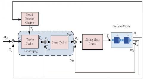
The backstepping-sliding structure for speed control incorporates an RBP-NN observer for a two-mas system, as shown in Figure 3.
In this section, the proposed adaptive controller is simulated in the Matlab/Simulink environment in comparison to the model-based technique to verify the accuracy and availability of the method. The Matlab/Simulink with parameters and coefficients:
$J_M=0.1 \mathrm{kgm}^2 ; J_L=0.01 \mathrm{kgm}^2 ; K_s=20 \mathrm{Nm} / \mathrm{rad}$
$\alpha=2 ; c_1=15 ; c_2=60 ; c_3=30 ; c_4=25$
Furthermore, the RBF neural network’s parameters are chosen as Neural number.
$n=25 ; \Gamma=\left[\begin{array}{ccc}3 & \cdots & 3 \\ \vdots & \ddots & \vdots \\ 3 & \cdots & 3\end{array}\right]_{n \times n} ; c=\operatorname{linspace}(-30,30, n) ; b=0.25$
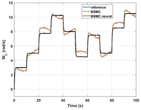
The simulation is conducted with a scenario when the load moment is an uncertain factor affected by an external noise of the system vibration. Therefore, the load moment is unknown for the model-based controller using backstepping aggregated with sliding mode control (BSMC). On the other hand, with an adaptive law designed based on the Lyapunov standard, the proposed RBF neural network can approximate an appropriate value for unknown factors even when it is affected by the bounded disturbance. Therefore, the higher control performance can be seen in the results of the BSMC combined with RBFNN (BSMC neural) in the following Figure 4 and Figure 5.
Figure 3. Structure backstepping- sliding speed-controlled incorporating neural network observer of a two-mass system
Figure 4. Angular load speed
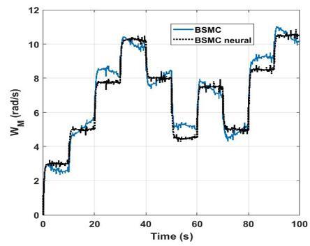
Figure 5. Angular motor speed
Figure 4 shows the responses of the two controllers compared to the reference value. It can be seen that BSMC neural controller generated an angular load speed that is considerably close to the desired value. However, the unknown factor combined with the disturbance exists in the system. Otherwise, these adverse elements significantly affect the BSMC performance when its load speed is quite different from the reference. Likewise, the angular motor speed results show the corresponding performance in Figure 5.
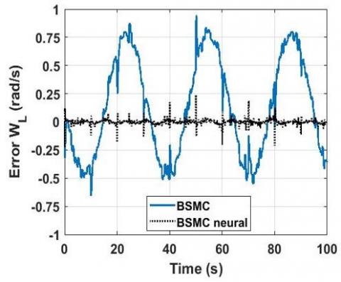
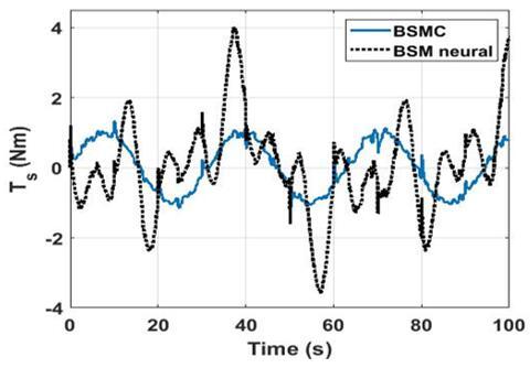
The load speed errors are shown in Figure 6, with the maximum value of about 0.9 rad/s of the BSMC method. Moreover, the BSMC’s number fluctuates according to the unknown load moment, while that of the neural-based controller constantly oscillates in an acceptable range around zero. Besides, motor and shaft torque responses are given in Figure 7 and Figure 8.
Figure 6. Angular load speed error
Figure 7. Motor torque
Figure 8. Shaft torque
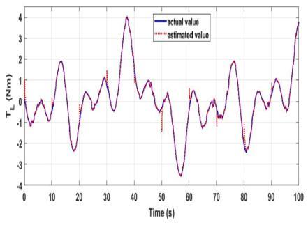
Figure 9 shows the approximated performance of the RBF neural network. In general, the output value keeps tracking the actual value throughout the considered period. Therefore, proper values of the load moment are continuously generated for the controller so that it can guarantee system stability.
Figure 9. Neural network output in comparison to the actual value
In this paper, the two-mass system with flexible couplings comprises an induction motor, and a load is considered. Backstepping-sliding mode control combined with RBFNN observer is employed to solve the speed control problem of the system. This control method controls the actual angular speed matching the angular reference speed of the motor and load. The simulation results show that high dynamic and suppression of the mechanical oscillation of the drive system can be achieved. The advantage over other methods is without the mathematical mode of two mass systems. Therefore, this torque observer design is more straightforward than the method design-based state mode of the system.
This research is sponsored by the project at the University of Transport and Communications.
[1] Łuczak, D. (2014). Mathematical model of multi-mass electric drive system with flexible connection. Conference: 2014 19th International Conference on Methods and Models in Automation and Robotics, MMAR, pp. 590-595. http://dx.doi.org/10.1109/MMAR.2014.6957420
[2] Ma, C.B., Hori, Y. (2004). Backlash vibration suppression control of torsional system by novel fractional order PID controller. IEEJ Transactions on Industry Applications, 124(3): 312-317. http://dx.doi.org/10.1541/ieejias.124.312
[3] Zhang, G., Furusho, J. (2000). Speed control of two-inertia system by PI/PID control. IEEE Transactions on Industrial Electronics, 47(3): 603-609. http://dx.doi.org/10.1109/41.847901
[4] Ikeda, H. (2018). PID controller design methods for multi-mass resonance system. PID Control for Industrial Processes. http://dx.doi.org/10.5772/intechopen.74298
[5] Thomsen, S., Fuchs, F.W. (2011). Design and analysis of a flatness-based control approach for speed control of drive systems with elastic couplings and uncertain loads. Proceedings of the 14th European Conference on Power Electronics and Applications, pp. 1-10.
[6] Ha, V.T., Quang, N.P. (2019). Flatness-based control design for two-mass system using induction motor drive fed by voltage source inverter with ideal control performance of stator current. Mechanisms and Machine Science, 70: 39-50. http://dx.doi.org/10.1007/978-3-030-13321-4_4
[7] Thomsen, S., Fuchs, F.W. (2010). Flatness based speed control of drive systems with resonant loads. IECON 2010 - 36th Annual Conference on IEEE Industrial Electronics Society, pp. 120-125. http://dx.doi.org/10.1109/IECON.2010.5675188
[8] Thanh Ha, V.T., Tan, L., Nam, N.D., Quang, N.P. (2019). Backstepping control of two-mass system using induction motor drive fed by voltage source inverter with ideal control performance of stator current. International Journal of Power Electronics and Drive Systems, 10(2): 720-730. https://doi.org/10.11591/IJPEDS.V10.I2.PP720-730
[9] Mola, M., Khayatian, A., Dehghani, M. (2013). Backstepping position control of two-mass systems with unknown backlash. 2013 9th Asian Control Conference (ASCC), pp. 1-6. http://dx.doi.org/10.1109/ASCC.2013.6606181
[10] Ikeda, H., Hanamoto, T. (2013). Fuzzy controller of multi-inertia resonance system designed by Differential Evolution. Electrical Machines and Systems (ICEMS), 2013 International Conference, 3(2): 2291-2295. http://dx.doi.org/10.1109/ICEMS.2013.6713239
[11] Korondi, P., HashUnot, H., Utkin,V. (1997). Sliding mode design for two mass system based on reduced order model. IFAC Proceedings Volumes, 30(16): 303-308. https://doi.org/10.1016/S1474-6670(17)42623-1
[12] Chaitanya, K.M.N., Reddy, K., Boddepalli, R., Sangameswara, P. (2016). Control of non linear two mass drive system using ANFIS. International Journal of Advanced Research in Electrical Electronics and Instrumentation Engineering, 5(12): 9214-9224. http://dx.doi.org/10.15662/IJAREEIE.2016.0512014
[13] Shahgholian, G., Faiz, J., Shafaghi, P. (2010). Analysis and simulation of speed control for two-mass resonant system. ICCEE 09: Proceedings of the 2009 Second International Conference on Computer and Electrical Engineering, 2: 666-670. https://doi.org/10.1109/ICCEE.2009.41
[14] Serkies, P. (2019). Estimation of state variables of the drive system with elastic joint using moving horizon estimation (MHE). Bulletin of the Polish Academy of Sciences Technical Sciences, 67(5). https://doi.org/10.24425/BPASTS.2019.130881
[15] Szabat, K., Than, T.V., Kamiński, M. (2015). A modified fuzzy luenberger observer for a two-mass drive system. IEEE Transactions on Industrial Informatics, 11(2): 531-539. http://dx.doi.org/10.1109/TII.2014.2327912
[16] Holten, L., Gjelsvik, A., Aam, S., Wu, F.F., Liu, W.H.E. (1988). Comparison of different methods for state estimation. IEEE Transactions on Power Systems, 3(4): 1798-1806. https://doi.org/10.1109/59.192998
[17] Park, J.H., Huh, S.H. Kim, S.H., Seo, S.J., Park, G.T. (2005). Direct adaptive controller for nonaffine nonlinear systems using selfstructuring neural networks. IEEE Transactions on Neural Networks, 16(2): 414-422. http://dx.doi.org/10.1109/TNN.2004.841786
[18] Rovithakis, G.A. (2004). Robust redesign of a neural network controller in the presence of unmodeled dynamics. IEEE Transactions on Neural Networks, 15(6): 1482-1490. https://doi.org/10.1109/tnn.2004.837782
[19] Talebi, H.A., Patel, R.V., Wong, M. (2002). A neural network based observer for flexible-joint manipulators. IFAC Proceedings Volumes, 35(1): 317-322. https://doi.org/10.3182/20020721-6-ES-1901.00865
[20] Shahgholian, G. (2013). Modeling and simulation of a two-mass resonant system with speed controller. International Journal of Information and Electronics Engineering, 3(5): 448-452. https://doi.org/10.7763/IJIEE.2013.V3.355
[21] Abdollahi, F., Talebi, H.A., Patel. R.V. (2006). A stable neural network-based observer with application to flexible-joint manipulators. IEEE Transactions on Neural Networks, 17(1). https://doi.org/10.1109/TNN.2005.863458
[22] Sioud, H., Sharafin, A., Eliker, K., Zhang, W.D. (2018). Chebyshev neural network observer based RBF neural network terminal sliding mode controller for a class of nonlinear system. Chinese Control and Decision Conference (CCDC), pp. 325-331. https://doi.org/10.1109/CCDC.2018.8407153