Aouiche Abdelaziz* | Aouiche El Moundher | Guiza Dhaouadi
© 2022 IIETA. This article is published by IIETA and is licensed under the CC BY 4.0 license (http://creativecommons.org/licenses/by/4.0/).
OPEN ACCESS
This paper addresses the performance of the Artificial Neural Networks (ANNs), Fuzzy inference systems (FISs) and Adaptive Neuro-Fuzzy Inference System (ANFIS) for the identification of some nonlinear systems with certain degree of uncertainty. The efficiency of the suggested methods in modeling and identification the responses were analyzed and compared. The Back-propagation algorithm and Takagi-Sugeno (TS) approach are used to train the ANNs, FISs and ANFIS, respectively. In this study we will show how ANFIS can be put in order to form nets that able to train from external data and information compared to ANNs and FISs. In order, it is proposed forms of inputs that can be used along with ANNs, FISs and ANFIS to modeling nonlinear systems. Two nonlinear systems with an electrocardiogram (ECG) signal in the form of simulation and complexity were used to test the identification of the structure presented. Because ANFIS has an inherent capacity to approximate unknown functions and to adjust the changes in inputs and parameters, it can be used to identify the proposed systems with a very high level of complexity. The results show that the ANFIS technique can provide the most ideal approximation when the right structures are employed.
nonlinear systems, ECG signal, fuzzy inference models, neural networks, neuro-fuzzy systems
In last years, the techniques of artificial intelligent have been successfully used as building blocks in the design of practically feasible identifiers for nonlinear systems [1, 2]. Extensive simulation studies have shown that with some prior information concerning unknown nonlinear systems to be analysed, such identifiers result in satisfactory performance [3].
In this paper, three methods based on Artificial Neural Networks (ANNs), Fuzzy inference systems (FISs) and Adaptive Neuro-Fuzzy Inference System (ANFIS) are presented for modeling and identification of nonlinear systems. However, a comparison of both techniques shows that ANFIS is relatively superior to the ANNs and FISs techniques.
The ANFIS merges the advantages of (FISs) and (ANNs) in a unique model. Rapid training, perfect clarification facilities in the form of meaningful fuzzy rules, the capacity to accept data and existing expert information about the problem, and perfect generalization capability features have made neuro-fuzzy systems very popular in recent years [4, 5].
The results of Hou et al. [6] showed that ANFIS is very effective to identify the nonlinear system. This method introduced one of the most nonlinear models often used based on the Hammerstein model [7]. Martins et al. [8] used the modified ANFIS in the identification of nonlinear system and compared it to the ordinary ANFIS while giving excellent performance. In case of adjusting the radius of a cluster center a T-S fuzzy model with perfect performance is used for this subject [9]. Manoj [10] developed an ANFIS controller to make an inverted pendulum very stable. In the recent paper of Karaboga and Kaya, the ANFIS is trained by using ABC algorithm for the solution of the real-world problem, the number of foreign visitors coming to Turkey from the USA, Germany, Bulgaria, France, Georgia, the Netherlands, England, Iran and Russia is estimated [11]. Jamshidi et al. [12] purposed an ANFIS method for modelling and identification of complex current as the main important element of the batteries in impedance state, their results showed that this method can have acceptable output for impedance modelling the batteries.
In this work intelligent efficient identification methods are proposed. We used the data of the Input and the output in order to determine a main model for the system. After that the error between the system and the output model will modelled which gives us a model for the error, our interest is in the unknown nonlinear systems as well the Electrocardiogram (ECG) signal who describes the electrical activity of the heart.
We organized this paper as follows: In section 2, the mathematical formulation of the problem is presented. Section 3 is interested to theoretical formulation of the ANNs, FISs and ANFIS models. We provide in section 4 our simulation results and discussion, of our proposed ANFIS method compared to (ANNs) and (FISs) approaches. The obtained simulation results demonstrated the performance of the suggested technique, so the last section discusses the main finding of this work.
In this paper we will consider two kinds of systems:
2.1 Discrete time system
Consider the nonlinear discrete time system described by:
$y(k+1)=f[y(k), u(k)]$ (1)
Our prime objective in this work is to find a model around the origin and prove how it can be implemented using our suggested methods. The function f is unknown so ANNs, FISs and ANFIS are used to identify it. The architecture of the network is carried out by Back-propagation algorithm in combination with Sugeno model.
When f in Eq. (1) is supposed unknown, such our model has to be learned using Input/Output pairs (y(k), u(k))$\rightarrow$y(k+1).
The estimation error e(k+1) is defined by:
$e(k+1) \equiv y(k+1)-\hat{y}(k+1) e(k+1)=f[y(k), u(k)]-\hat{f}[\hat{y}(k), u(k)]$ (2)
To converge the error, the parameters of ANNs, FISs and ANFIS must be adjusted. This issue will be presented in the next Section. f can be obtained off-line only by the choice of suitable inputs u(k) and observation of the corresponding state y(k+1) as presented in Figure 1.
Figure 1. Architecture for estimation of f
2.2 Mathematical modeling of Electrocardiogram
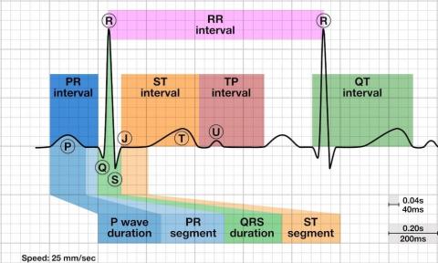
The Electrocardiogram (ECG) is a noninvasive recording of the electrical activity of the heart [13]. The ECG signal is obtained by depolarization and repolarization of atrial and ventricular muscles of the heart [14].
Figure 2. Trace ECG
As we can see from Figure 2 that the ECG signal has the following characteristics:
The ECG signal is quasi-periodic with fundamental frequency defined by heart rate, it also verifies the conditions of Dirichlet given by the following points:
The cardiac event can be classified to different main factors. The P wave, PR interval, Q wave, QRS complex, ST segment, T and U wave. Each of these portions signifies the electrical activity of the heart over the heartbeat period [15].
We know that any periodic functions verify the conditions of Dirichlet can be presented as a series of sinus and cosinus terms of frequencies, which comes to be a multiple of fundamental frequency. This information allows us to use the development of Fourier series by tranche on the ECG signal [16].
$f(x)=\frac{a_{0}}{2}+\sum_{n=1}^{\infty} \frac{a_{n} \cos (n \pi x)}{l}+\sum_{n=1}^{\infty} \frac{b_{n} \sin (n \pi x)}{l}$ (3)
$a_{0}=\frac{1}{l} \int_{0}^{T} f(x) d x \quad T=2 l$
$a_{n}=\frac{1}{l} \int_{0}^{T} f(x) \cos \left(\frac{n \pi x}{l}\right) d x \quad n=1,2,3$
$b_{n}=\frac{1}{l} \int_{0}^{T} f(x) \sin \left(\frac{n \pi x}{l}\right) d x \quad n=1,2,3$
2.3 Calculation
Each important characteristic of ECG signal can be represented by shifted and scaled.
Once we product each of these pats, they can be finally summed to obtain the ECG signal [17].
2.3.1 P wave
The P wave is assimilated to a cosine function which can be given by:
$f(x)=\left\{\begin{array}{cc}0 & -l<x<-l / b \\ \cos \left(\frac{\pi b}{2 l}\right) & -l / b<x<-l / b \\ 0 & l / b<x<l\end{array}\right.$ (4)
where
b: is an adjustment coefficient related to the duration of the wave.where
So, we can evaluate the coefficients of Fourier series as:
$a_{0}=1 / l \int \cos \left(\frac{\pi b x}{2 l}\right) d x$ (5)
So, $a_{0}=-4 / \pi b$.
$a_{n}=1 / l \int \cos \left(\frac{\pi b x}{2 l}\right) \cos \left(\frac{\pi b x}{l}\right) d x$ (6)
We find:
$a_{n}=\frac{2}{\pi(b-2 n)}(\sin (\pi b-2 n \pi) / 2 b)+\frac{2}{\pi(b-2 n)}(\sin (\pi b+2 n \pi) / 2 b)$ (7)
$b_{n}=1 / l \int \cos \left(\frac{n \pi x}{2 l}\right) \sin \left(\frac{n \pi x}{l}\right) d x$ (8)
As the function is pair so:
$b_{n}=0$
2.3.2 QRS complex
The QRS wave is assimilated to a triangular function which can be given by the following equation:
$f(x)=\left\{\begin{array}{cc}\left(-\frac{b a x}{l}\right)+a & 0<x<l / b \\ \left(-\frac{b a x}{l}\right)+a & -l / b<x<0\end{array}\right.$ (9)
So, we can evaluate the coefficients of Fourier series as:
$a_{0}=1 / l \int f(x) d x$ (10)
So $a_{0}=a / b$.
$a_{n}=1 / l \int f(x) \cos \left(\frac{\pi b x}{l}\right) d x$ (11)
where
$a_{n}=\frac{2 b a}{n^{2} \pi^{2}}\left(1-\cos \left(\frac{n \pi}{b}\right)\right)$ (12)
and
$b_{n}=1 / l \int f(x) \sin \left(\frac{n \pi x}{l}\right) d x$ (13)
As the function is pair so: bn=0.
Also, the generation of the waves (t, u, s) takes place in the same way as the preceding waves [18].
The three methods used are:
3.1 Artificial Neural Networks (ANNS)
Neural networks are a very robust method in order to construct hard and nonlinear systems [19]. There are various models of neural networks for many applications are popularly used today:
The most basic deep neural network often used is Multi-Layer Perceptron (MLP NN) architecture which in this work was used to identify the unknown functions. As shown in Figure 3 below, the MLP NN is composed of three layers: one or more hidden layers, vi are placed between the input and the output layer [20].
Figure 3. General Structure of MLP NN
Each neuron of layer hidden j adds up its input Ii when they are adjusted with the corresponding connections wij from the input layer and calculates its response Oj by the function f as:
$O_{j}=f\left(\sum w_{i j} I_{i}\right)$ (14)
f can be any type of activation functions. Learning MLP consists in adjusting its weights to provide a smaller margin of error on the training data, using a very successful method in practice called the Back-propagation algorithm.
The learning algorithm gives the change Dwij(k) in the weight of neuron between i and j [21].
The Back-propagation algorithm for the weights in the linear output layer becomes:
$w_{i j}(n e w)=w_{i j}($ old $)-\mu \frac{\partial e^{2}}{\partial w_{i j}}($ old $)$ (15)
where, e the error between original and obtained output of the neuron i, μ is a convergence factor, which may be different for each weight. Back-propagation algorithm uses exactly the strategy of gradient descent for adaptation as the Least Mean Squares (LMS) algorithm, and so it reduces to the LMS algorithm for neurons without any nonlinearity [22].
The algorithm implemented in this paper is the Back-propagation for both neural networks and fuzzy inference system, because of prominent advantages:
3.2 Fuzzy Inference Systems (FISs)
The important part of the Fuzzy Inference Systems (FISs) is the basic information about fuzzy rules.
Firstly, fuzzy IF-THEN rules must be collected from human experts or field knowledge [24]. FISs are constituted four different steps: fuzzification, weighting, generation and defuzzification.
Fuzzy models consist into three models:
1-Mamdani model: y=A (A is a fuzzy number).
2-Takagi-Sugeno model (TS) model: $y_{j}^{i}=f_{j}^{i}(x)$ (x is an input variable).
3-Simplified fuzzy model y=c (c is a constant).
IF the speed x of a car is slow; THEN the force to the accelerator is:
$y_{j}^{i}=f_{j}^{i}(x)=y_{j 0}^{i}+y_{j 1}^{i} x_{1}+y_{j 2}^{i} x_{2}+\cdots+y_{j p}^{i} x_{p}$ (16)
Because each rule is linearly dependent on the input variables, the TS method is perfect and suitable for modeling nonlinear systems by interpolating between multiple linear models. That’s why for all simulations in this study, we used the Sugeno model (singleton pattern) for identifying our nonlinear systems [26].
From Eq. (16), the final output of the system is given by:
$y=\hat{f}(\underline{x})=\frac{\sum_{l=1}^{M} \omega_{l} b_{l}}{\sum_{l=1}^{M} \omega_{l}}$
So
$y=\hat{f}(\underline{x})=\frac{\sum_{l=1}^{M} b_{l} \prod_{i=1}^{n} \exp \left(-\left(\frac{x_{i}-c_{i}^{l}}{\sigma_{i}^{l}}\right)^{2}\right)}{\sum_{l=1}^{M} \prod_{i=1}^{n} \exp \left(-\left(\frac{x_{i}-c_{i}^{l}}{\sigma_{i}^{l}}\right)^{2}\right)}$ (17)
where
$\omega_{l}=\mu_{A_{1}^{i}}\left(x_{1}\right) \wedge \ldots \wedge \mu_{A_{p}^{i}}\left(x_{p}\right)$ is the degree of verity of the lth rule and $\mu_{A_{j}^{i}}\left(x_{j}\right)$ is the membership degree of value xj to fuzzy set $A_{j}^{i}$. From Eq. (17), a Gaussian function is chosen by the term of exponential. The error between the original output and the fuzzy model is given by $e=\frac{1}{2}\left(O_{r}-\hat{f}(\underline{x})\right)^{2}$.
As we focused in our work on the Back-propagation algorithm of fuzzy models. The modified parameters: part of consequent bl, mean part of antecedent $c_{i}^{l}$, and sigma part of antecedent $\sigma_{i}^{l}$ are presented as:
$b^{l}(k+1)=b^{l}(k)+\alpha_{b} \frac{e}{B} \omega_{l}$ (18)
$c_{i}^{l}(k+1)=c_{i}^{l}(k)+\alpha_{c} \frac{(d-\hat{f})}{B}\left(b^{l}-\hat{f}\right)^{2} \frac{\left(x_{i}-c_{i}^{l}\right)}{\sigma_{i}^{l^{2}}} \omega_{l}$ (19)
$\sigma_{i}^{l}(k+1)=\sigma_{i}^{l}(k)+\alpha_{\sigma} \frac{e}{B}\left(b^{l}-\hat{f}\right)^{2} \frac{\left(x_{i}-c_{i}^{l}\right)}{\sigma_{i}^{l^{2}}} \omega_{l}$ (20)
where, αn(n=b,c,σ) is the learning rate and $B=\sum_{l=1}^{M} \omega_{l}$.
The training Back-propagation algorithm is shown in Eq. (18) Eq. (19), and Eq. (20).
For updating the parameters bl, the normalized error e/B is back-propagated to the layer bl then it’s modified by Eq. (18) when ωl is the input of bl.
For updating the parameters $c_{i}^{l}$ and $\sigma_{i}^{l}$, the normalized error adjusts $\left(b^{l}-\hat{f}\right)$ then ωl is backpropagated to the unit of processing of layer l; then $c_{i}^{l}$ and $\sigma_{i}^{l}$ are modified by Eq. (19) and Eq. (20) [27].
We used in this paper the series-parallel identification model in which the output of the nonlinear plant (rather than the identification model) is fed back into the identification model. Because we only use the series-parallel identification model, the static Back propagation algorithm developed is sufficient to train the identifiers.
3.3 Adaptive Network-Based Fuzzy Inference System (ANFIS)
In this section, we show a kind of adaptive networks who are similar to fuzzy inference systems previously cited.
The combination of ANNs and FISs approaches has resulted a powerful and rapid technic called Adaptive Neuro-Fuzzy Inference System (ANFIS), adopted and considered to solve real problems [28].
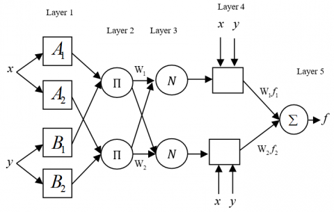
Figure 4 presents an architecture of ANFIS with the fuzzy inference system has two inputs x and y and one output f. We consider that the rule base has two fuzzy IF-THEN rules using Takagi and Sugeno [29] approach:
Rule 1:
If $x$ is $A_{1}$ and $y$ is $B_{1}$, THEN $f_{1}=p_{1} x+q_{1} y+r_{1}$
Rule 2:
If $x$ is $A_{2}$ and $y$ is $B_{2}$, THEN $f_{2}=p_{2} x+q_{2} y+r_{2}$
A five-layer neuro-fuzzy network is used to reach the function f.
Figure 4. ANFIS Architecture with two inputs
About network's training, there are two passes, a forward and backward one. The first pass propagates the input vector by the network layer by layer. For backward pass, the error is sent back into the network every time in a same manner to Back-propagation [30, 31].
We check that our models after training are able in fact to identify the original response for values yielded in the input that are not employed in training step.
4.1 Proposed systems
The second-order recurrent equation is described by:
$y(k+1)=f[y(k), y(k-1)]+u(k)$ (21)
where the unknown function f has the form:
$f[y(k), y(k-1)]=\frac{y(k) y(k-1)[y(k)+2.5]}{\left(1+y(k)^{2}+y(k-1)^{2}\right.}$
In order to identify:
$y(k+1)=\hat{f}[y(k), y(k-1)]+u(k)$
The MISO system to be identified is presented by the recurrent equation:
$y(k+1)=f[y(k), y(k-1), y(k-2), u(k), u(k-1)]$
where the unknown function f has the form:
$\hat{f}[y(k), y(k-1), y(k-2), u(k), u(k-1)]=\frac{[y(k) y(k-1) y(k-2) u(k-1)][y(k-2)-1]+u(k)}{1+y(k-2)^{2}+y(k-1)^{2}}$
To identify:
$y(k+1)=\hat{f}[y(k), y(k-1), y(k-2), u(k), u(k-1)]$
4.2 ECG signal
We propose here to identify a nonlinear ECG signal with a period p as a dynamical model by the following equation:
$f(x)=\widehat{E C G}[x+n p]$, n=1,2,...
The Fourier series of a periodic function f(x) of period 2l in the interval (-l, l) is given by Eq. (3).
Table 1. Different characteristics of normal ECG
|
Characteristics |
Values |
||
|
Wave P |
Duration (s) |
0.06-0.11 |
|
|
Amplitude (mm) |
˂2 |
||
|
Complex QRS |
Duration (s) |
0.05 - 0.10 |
|
|
Amplitude (mm) |
Q |
<25% of R |
|
|
R |
<5 |
||
|
S |
<20 |
||
|
Wave T |
Duration (s) |
020-0.25 |
|
|
Amplitude (mm) |
>-3 and <4 |
||
|
Wave U |
Amplitude (mm) |
<0.5 |
|
Table 1 summarizes the different parameters values of normal ECG, if their values are outside these intervals therefore the signal is abnormal [32].
Table 2 presents the architecture of our ANFIS Model for system 1, system 2 and the ECG signal compared to ANNs and FISs models:
For system 1 we chose a reference model described by the second-order recurrent equation:
$y_{m}(k+1)=0.6 y_{m}(k)+0.2 y_{m}(k-1)+r(k)$
where, r(k) is abounded reference input:
$r(k)=\sin \left(\frac{2 \Pi k}{2.5}\right)$
If the output error e(k) is defined as e(k)=yp(k)=ym(k) such that $\lim _{k \rightarrow \infty} e(k)=0$.
For system 2 to ensure that our model always follows the original system, we applied an input on two intervals (1≤k≤800):
$u(k)=\sin \left(\frac{2 \pi k}{250}\right) \quad \quad$ For $1 \leq k \leq 500$
$u(k)=0.8 \sin \left(\frac{2 \pi k}{250}\right)+0.2 \sin \left(\frac{2 \pi k}{25}\right) \quad 500 \leq k \leq 800$
Finally, Figure 7 presents a fuzzy-neuro model of an ECG signal (ECG).
In this work, we employed the decomposed characteristics of fuzzy set models through the Neuro-Fuzzy system for the identification of our suggested nonlinear systems, include the ECG signal.
For testing the robustness of our suggested approaches, we choose three criterions of quality; training time, number of iterations and the Mean Square Error (MSE) between our estimated models and the desired outputs, as shown in Table 2.
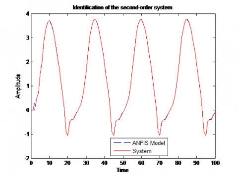
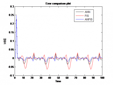
We see from Figure 5(a) that our ANFIS identifier with two inputs follows the desired system 1, as shown in Figure 5(b) the Mean Square Error (MSE) between our model and the original system equal to 6.1634e-005, 6.726e-004 and 4.7050e-04 for ANNs and FISs identifiers, respectively applying any values of the inputs suitable to their prescribed domain of variations, so it seems that the ANFIS identifier achieved better performance than ANNs and FISs identifiers.
The Figure 6(a) shows the simulation results of system 2 with five inputs. The MSE tends to 7.7849e-05 for ANFIS, 4.2842e-04 and 0.0014 for ANNs and FISs, respectively as shown in Figure 6(b), even the entire number of inputs increased to five, always neuro-fuzzy model trained to obtain better performances than ANNs and FISs.
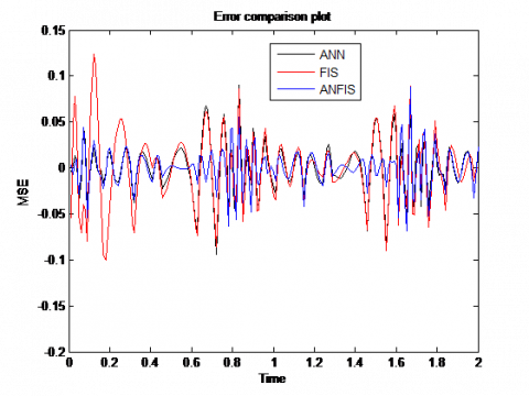
The Figure 7(a) shows the identification results of a normal ECG signal which we have an unknown function $\widehat{E C G}$. As seen in the Table 2, the MSE between our ANFIS model and the desired ECG signal shows always the Neuro-fuzzy model (ANFIS) achieved better performance than the other identifiers however the number of inputs increased to seven.
Table 2. ANNs, FISs and ANFIS architectures used to identify the outputs of proposed systems
|
Model Process |
System 1 |
System 2 |
ECG Signal |
|
|
ANNs |
Output Structure |
$\hat{f}$ |
$\widehat{E C G}$ |
|
|
Number of hidden layers |
2 |
|||
|
Algorithm |
Back-propagation |
|||
|
First hidden layer |
20 neurons |
40 |
||
|
Second hidden layer |
10 neurons |
20 |
||
|
Activation function |
sigmoid |
|||
|
Adjusted Gain |
0.1 |
0.9 |
||
|
Random input |
[-2,2] |
[0.1,5] |
||
|
Training time (S) |
1310 |
2347.3 |
3480 |
|
|
Number of iterations |
10000 |
21000 |
30000 |
|
|
MSE |
6.7267e-04 |
4.2842e-04 |
8.0624e-04 |
|
|
FISs
|
Number of rules |
20 |
30 |
|
|
Algorithm |
Back-propagation |
|||
|
Random input |
[-2,2] |
[-1,1] |
[0.1,5] |
|
|
Part of consequent $\alpha_{c}$ |
0.9 |
1 |
0.5 |
|
|
Part of premise $\alpha_{b}$ |
0.4 |
0.5 |
0.1 |
|
|
Sigma part of antecedent $\delta$ |
0.9 |
0.5 |
0.9 |
|
|
Training time (s) |
967.4380 |
1607.6 |
9422 |
|
|
Number of iterations |
6000 |
7000 |
18000 |
|
|
MSE |
4.7050e-04 |
0.0014 |
4.1701e-04 |
|
|
ANFIS |
Fuzzy rules number |
9 |
32 |
128 |
|
Training input victor |
2 |
5 |
7 |
|
|
Number of nodes |
35 |
92 |
294 |
|
|
Number of linear parameters |
27 |
192 |
1024 |
|
|
Number of nonlinear parameters |
18 |
30 |
42 |
|
|
Total number of parameters |
45 |
222 |
1066 |
|
|
Number of training data pairs |
100 |
200 |
||
|
MSE |
6.1634e-005 |
7.7849e-05 |
1.8362e-05 |
|
(a)
(b)
Figure 5. (a) Fuzzy-Neural Model and desired system 1, (b) MSE between ANNs, FISs and ANFIS
(a)
(b)
Figure 6. (a) Fuzzy-Neural Model and desired system 2, (b) MSE between ANNs, FISs and ANFIS
(a)
(b)
Figure 7. (a) Fuzzy-Neural Model and original ECG, (b) MSE between ANNs, FISs and ANFIS
This paper represents perfect approaches for identification and modeling of nonlinear systems. The identification of some systems with different complexity and an ECG signal are done using three different technics; the Neural Networks, Fuzzy systems and hybrid Neuro-fuzzy networks. As shown in Figure 5 (b), Figure 6 (b) and Figure 7 (b) (comparison of training curves between ANNs, FISs and ANFIS), hybrid network provides a better error reduction, decreased number of iterations and short training time compared to the other models whatever the number of inputs as illustrated for ECG signal. Due to short processing time and higher accuracy of the proposed method, Neuro-fuzzy model can be used as a real-time arrhythmia identification system. Higher accuracy of the system makes it highly reliable and efficient.
[1] Phan, M.Q., Juang, J.N., Hyland, D.C. (1995). On neural networks in identification and control of dynamic systems. In Wave Motion, Intelligent Structures and Nonlinear Mechanics, 194-225. https://doi.org/10.1142/9789812796455_0007
[2] Bolcskei, H., Grohs, P., Kutyniok, G., Petersen, P. (2019). Optimal approximation with sparsely connected deep neural networks. SIAM Journal on Mathematics of Data Science, 1(1): 8-45. https://doi.org/10.1137/18M118709X
[3] Sada, S.O., Ikpeseni, S.C. (2021). Evaluation of ANN and ANFIS modeling ability in the prediction of AISI 1050 steel machining performance. Heliyon, 7(2): e06136. https://doi.org/10.1016/j.heliyon.2021.e06136.
[4] Jang, J.S. (1993). ANFIS: adaptive-network-based fuzzy inference system. IEEE Transactions on Systems, Man, and Cybernetics, 23(3): 665-685. https://doi.org/10.1109/21.256541
[5] Jang, J.S.R., Sun, C.T., Mizutani, E. (1997). Neuro-fuzzy and soft computing-a computational approach to learning and machine intelligence. Pearson College Div; US Ed edition.
[6] Hou, Z., Shen, Q., Li, H. (2003). Nonlinear system identification based on ANFIS. In International Conference on Neural Networks and Signal Processing, 1: 510-512. https://doi.org/10.1109/ICNNSP.2003.1279323
[7] Cuevas, E., Díaz, P., Avalos, O., Zaldivar, D., Pérez-Cisneros, M. (2018). Nonlinear system identification based on ANFIS-Hammerstein model using Gravitational search algorithm. Applied Intelligence, 48(1): 182-203. https://doi.org/10.1007/s10489-017-0969-1
[8] da Costa Martins, J.K.E., de Araújo, F.M.U. (2015). Nonlinear system identification based on modified ANFIS. In 2015 12th International Conference on Informatics in Control, Automation and Robotics (ICINCO), 1: 588-595.
[9] Yue, J., Liu, J., Liu, X., Tan, W. (2006). Identification of nonlinear system based on ANFIS with subtractive clustering. In 2006 6th World Congress on Intelligent Control and Automation, 1: 1852-1856. https://doi.org/10.1109/WCICA.2006.1712675
[10] Manoj, S.B.A. (2011). Identification and control of nonlinear systems using soft computing techniques. International Journal of Modeling and Optimization, 1(1): 24.
[11] Karaboga, D., Kaya, E. (2020). Estimation of number of foreign visitors with ANFIS by using ABC algorithm. Soft Computing, 24(10): 7579-7591. https://doi.org/10.1007/s00500-019-04386-5
[12] Jamshidi, M., Farhadi, R., Jamshidi, M., Shamsi, Z., Naseh, S. (2020). Using a soft computing method for impedance modelling of li-ion battery current. International Journal of Advanced Intelligence Paradigms, 16(1): 18-29. https://doi.org/10.1504/IJAIP.2020.106686
[13] Goldberger, A.L. (2006). Clinical Electrocardiography: A Simplified Approach. e (7th ed.). Mosby–Elsevier.
[14] Kher, R. (2019). Signal processing techniques for removing noise from ECG signals. J. Biomed. Eng. Res, 3(101): 1-9.
[15] Diker, A., Engin, A.V.C.I. (2019). Feature extraction of ECG signal by using deep feature. In 2019 7th International Symposium on Digital Forensics and Security (ISDFS), pp. 1-6. https://doi.org/10.1109/ISDFS.2019.8757522
[16] Shobana, R., Pavithra, J. (2021). Fourier series in electrocardiograph. International Journal of Mathematics Trends and Technology, 67(5): 95-100. https://doi.org/10.14445/22315373/IJMTT-V67I5P511
[17] Panigrahy, D., Sahu, P.K. (2018). P and T wave detection and delineation of ECG signal using differential evolution (DE) optimization strategy. Australasian Physical & Engineering Sciences in Medicine, 41(1): 225-241. https://doi.org/10.1007/s13246-018-0629-8
[18] Khandpur, S. (2014). Handbook of Biomedical Instrumentation. MC GRAW HILL INDIA; 3rd Revised edition.
[19] Goodfellow, I., Pouget-Abadie, J., Mirza, M., Xu, B., Warde-Farley, D., Ozair, S., Bengio, Y. (2014). Generative adversarial nets. Advances in Neural Information Processing Systems, 27. https://doi.org/10.1145/3422622
[20] Agrawal, S.K. (2021). Understanding the basics of artificial neural network. Data Science Blogathon. https://www.analyticsvidhya.com/blog/2021/07/understanding-the-basics-of-artificial-neural-network-ann/.
[21] Übeylı, E.D., Güler, İ. (2004). Multilayer perceptron neural networks to compute quasistatic parameters of asymmetric coplanar waveguides. Neurocomputing, 62: 349-365. https://doi.org/10.1016/j.neucom.2004.04.005
[22] Abirami, S., Chitra, P. (2020). The digital twin paradigm for smarter systems and environments: The industry use cases. In Adavances in Computers.
[23] Vlachas, P.R., Pathak, J., Hunt, B.R., Sapsis, T.P., Girvan, M., Ott, E., Koumoutsakos, P. (2020). Backpropagation algorithms and reservoir computing in recurrent neural networks for the forecasting of complex spatiotemporal dynamics. Neural Networks, 126: 191-217. https://doi.org/10.1016/J.Neunet.2020.02.016
[24] Wang, L.X. (1997). A course in fuzzy systems and control. Prentice Hall, Upper Saddle River. New Jersey.
[25] Takagi, H. (1997). Introduction to fuzzy systems, neural networks, and genetic algorithms. In Intelligent Hybrid Systems, 3-33. Springer, Boston, MA. https://doi.org/10.1007/978-1-4615-6191-0_1
[26] Mizumoto, M. (1996). Product-sum-gravity method= fuzzy singleton-type reasoning method= simplified fuzzy reasoning method. In Proceedings of IEEE 5th International Fuzzy Systems, 3: 2098-2102. https://doi.org/10.1109/FUZZY.1996.552786
[27] Wang, L.X., Mendel, J.M. (1992). Back-propagation fuzzy system as nonlinear dynamic system identifiers. In IEEE International Conference on Fuzzy Systems, pp. 1409-1418. https://doi.org/10.1109/FUZZY.1992.258711
[28] Zhang, C., Sun, J., Wang, Q., Feng, Z. (2007). A novel GA-LM based hybrid algorithm. In Third International Conference on Natural Computation, 2: 479-483. https://doi.org/10.1109/ICNC.2007.112
[29] Takagi, T., Sugeno, M. (1983). Derivation of fuzzy control rules from human operator's control actions. IFAC Proceedings Volumes, 16(13): 55-60. https://doi.org/10.1016/S1474-6670(17)62005-6
[30] Weigend, A.S., Rumelhart, D.E., Huberman, B.A. (1991). Back-propagation, weight-elimination and time series prediction. In Connectionist Models, 105-116. https://doi.org/10.1016/B978-1-4832-1448-1.50016-0
[31] Takagi, T., Sugeno, M. (1985). Fuzzy identification of systems and its applications to modeling and control. IEEE Transactions on Systems, Man, and Cybernetics, 15(1): 116-132. https://doi.org/10.1109/TSMC.1985.6313399
[32] Angelov, P.P., Filev, D.P. (2004). An approach to online identification of Takagi-Sugeno fuzzy models. IEEE Transactions on Systems, Man, and Cybernetics, Part B (Cybernetics), 34(1): 484-498. https://doi.org/10.1109/TSMCB.2003.817053