Abderrahmane Benabbas* | Elyazid Zaidi | Rachid Abdessemed
© 2022 IIETA. This article is published by IIETA and is licensed under the CC BY 4.0 license (http://creativecommons.org/licenses/by/4.0/).
OPEN ACCESS
In this work, the modeling and the sliding mode control of a self-excited asynchronous generator integrated in a wind energy conversion system is studied. The dc-link voltage and frequency output by the wind turbine depend on the wind intensity applied to the turbine and load. The goal of the study is to increase energy quality and to achieve a stabilization of dc-link voltage and frequency values based on sliding mode control. This method offers stability and robustness against external disturbances. However, this method is based in the power converter to improve the excellent dynamic of wind energy conversion system to meet the connection to the main grid. The simulation results show the efficiency and reliability of the proposed control method.
asynchronous cage generator, wind turbine, sliding mode control, rectifier
The production of electricity by wind turbines depends mainly on the strength of the wind at a given time. Wind energy is an undegradable renewable energy [1, 2]. Moreover, it is an energy which does not produce any atmospheric discharge or radioactive waste. However, wind speed is variable, a wind turbine cannot be set at its optimum permanently [3]. Operating the wind turbine around optimal point can maximize the power extracted from the wind during its variation [4]. This technique of Maximum Power Point Tracker (MPPT) consists of adjusting the electromagnetic torque to fix the speed at a reference value ωref.
An Induction generator with a squirrel-cage rotor, more commonly called self-excited generator, is a popular generator widely used in AC generators because it is robust, unexpensive and being mostly used in high power applications. It is able to limit the short-circuit current [5]. However, if most generators require external excitation, the cage generator requires a bank of stator capacitors for its excitation. The static converters (rectifier and inverter) are intermediate between the generator and the network (the load). The sliding mode control strategy is used to increase the performance and the quality of the produced energy [6-8].
Adjustment by sliding mode is a particular operating technique for systems with variable structure. The theory of systems with variable structure and associated sliding modes is a non-linear control technique. It is characterized by control discontinuity at the transition between switching surfaces called sliding surfaces [9, 10].
The sliding mode technique consists of bringing the trajectory of a system state towards the sliding surface and having it switched using an appropriate commutation around it until the equilibrium point [11].
In the beginning, this study is focused on the modeling and control of a self-excited asynchronous generator. It can be considered as the continuation of the work of Yang [12]. We consider the same technical solution, i.e. to develop a new mathematical model for the control of the self-excited asynchronous generator. Subsequently, we were also interested in the control of a system by sliding mode.
The work is organized as follows: In section 2, the studied system is presented and explained. In the next Section, we explain the application of the wind turbine using sliding mode controller based on the asynchronous cage generator. In section 4, the main simulation results are presented. Finally, a general conclusion is given in the last section.
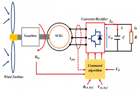
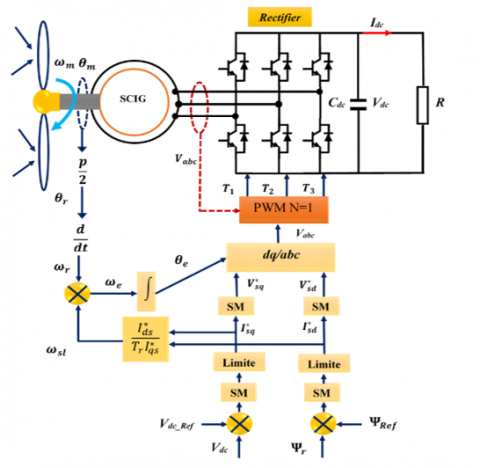
An aero-generator (Figure 1), more commonly known as a wind turbine, is a device that transforms part of the kinetic energy of the wind into mechanical energy available on a transmission shaft, then into electrical energy via an asynchronous cage generator and two static converters (rectifier, inverter) [12-14].
Figure 1. Schematic diagram of the system studied
2.1 Turbine modeling
The incoming wind power pv:
pv=12ρsV31 (1)
with:
ρ : air density (kg/m³);
Cp : power coefficient;
s: surface swept by the blades. (m2);
V1: upstream wind speed (m/s).
The mechanical power pm available on the shaft of an aerogenerator is thus expressed [15-17].
Pm=12ρsCp(λ)V31 (2)
with:
Cp=PmPv (3)
and:
λ=ΩturrV1 (4)
with:
Ωtur : rotational speed of the wind turbine;
γ : blade radius (mm).
The maximum value of Cp is reached when:
CPmax
It is this theoretical limit, called the Betz limit, that fixes the maximum extractable power for a given wind speed [18]. Therefore, the maximum extracted power is:
P_{m_{\max }}=\frac{1}{2} \rho S C_{P_{\max }} V_{1}^{3} (5)
The turbine torque is:
C_{a e r}=\frac{P_{m}}{\Omega_{t u r}}=\frac{1}{2 \Omega_{t u r}} \rho S C_{p}(\lambda) V_{1}^{3} (6)
and:
\Omega_{m e c}=G \Omega_{t u r} (7)
with:
\Omega_{\text {mec }}: angular speed of the generator(rad/s);
G: gain of the multiplier.
The mechanical torque on the generator shaft is:
C_{m e c}=\frac{1}{G} C_{a e r} (8)
The generator tree is modeled by the following equation:
J_{T} \frac{d \Omega_{m e ́ c}}{d t}=C_{T}-C_{V i s} (9)
The viscous friction torque is modeled by:
C_{V i s}=f_{T} \Omega_{m e ́ c} (10)
The total torque of the wind turbine is given by:
C_{T}=C_{m e ́ c}-C_{e m} (11)
J_{T}=\frac{J_{\text {turbine }}}{G^{2}}+J_{g} (12)
with:
C_{e m} : electromagnetic torque (N.m);
J_{T}: total inertia of rotating parts \left(k g \cdot m^{-3}\right);
f_{T} : total viscous friction coefficient (N.m.s/rd);
J_{g} : generator inertia (kg.m2).
2.2 The maximum power extraction techniques
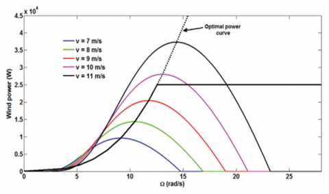
The power captured by the wind turbine can be essentially maximized by adjusting the coefficient C_{p}. The use of a variable speed wind turbine allows maximizing this power by the Maximum Power Point Tracking (M.P.P.T). Let us consider the behavior of an MPPT for a wind energy conversion system. The MPPT command allows to position the system at the optimum power point regardless of wind speed (Figure 2) [19].
Figure 2. Extraction of maximum power for different wind speeds
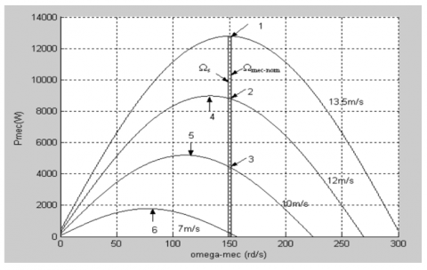
To maximize power, when the wind speed is lower than its nominal value, the mechanical speed of the wind turbine corresponds to points 4, 5 and 6 [19] (Figure 3).
Figure 3. Characteristic (power - mechanical speed)
2.3 Modeling of the self-excited asynchronous generator
The Park equations of the machine in the frame of the rotating field [19, 20]:
V_{s d}=R_{s} i_{s d}+\frac{d \psi_{s d}}{d t}-w_{s} \psi_{s q} (13)
V_{s q}=R_{s} i_{s q}+\frac{d \psi_{s q}}{d t}+w_{s} \psi_{s d} (14)
0=R_{r} i_{r d}+\frac{d \psi_{r d}}{d t}-w_{s l} \psi_{r q} (15)
0=R_{r} i_{r q}+\frac{d \psi_{r q}}{d t}+w_{s l} \psi_{r d} (16)
With:
\left(V_{s d}\right. and \left.V_{s q}\right): stator voltages on the axes (d,q)(V);
\left(i_{s d}\right. and \left.i_{s q}\right): stator currents on the axes (d,q)(A);
\left(i_{r d}\right. and \left.i_{r q}\right): rotor currents on the axes (d,q)(A);
\left(\psi_{s d}\right. and \left.\psi_{s q}\right): stator fluxes on the axes (d,q)(Wb);
\left(\psi_{r d}\right. and \left.\psi_{r q}\right): rotor fluxes on the axes (d,q)(Wb);
\mathrm{W}_{\mathrm{Sl}}=\mathrm{W}_{\mathrm{S}}-\mathrm{W}: sliding speed(rad);
\mathrm{W}_{\mathrm{S}}: rotating field speed(rad/s);
w: rotor speed(tr/mn);
R_{S}: stator resistance (\Omega);
R_{r}: rotor resistance (\Omega).
The flux is given by:
\left\{\begin{array}{l}\psi_{s d}=L_{s} I_{s d}+L_{m} I_{r d}=L_{\sigma s} I_{s d}+\psi_{m d} \\ \psi_{s q}=L_{s} I_{s q}+L_{m} I_{r q}=L_{\sigma s} I_{s q}+\psi_{m q}\end{array}\right. (17)
\left\{\begin{array}{l}\psi_{r d}=L_{r} I_{r d}+L_{m} I_{s d}=L_{\sigma r} I_{r d}+\psi_{m d} \\ \psi_{r q}=L_{r} I_{r q}+L_{m} I_{s q}=L_{\sigma r} I_{r q}+\psi_{m q}\end{array}\right. (18)
where,
\psi_{m}: magnetizing flux, \psi_{m}=L_{m} I_{m};
I_{m} : magnetizing current;
\psi_{m d}=L_{m} I_{m d}, \psi_{m q}=L_{m} I_{m q};
L_{S}: stator inductance (mH);
L_{r} : rotor inductance (mH);
L_{m}: magnetization inductance (mH);
L_{\sigma S} : stator leakage inductance [mH);
L_{\sigma r}: rotor leakage inductance (mH).
\left\{\begin{array}{l}I_{m d}=I_{s d}+I_{r d} \\ I_{m q}=I_{s q}+I_{r q}\end{array}\right. (19)
I_{m}=\sqrt{I_{m d^{2}}+I_{m q^{2}}} (20)
The synchronous electromagnetic torque developed by the rotating field is given by the following expression [19]:
C_{e m}=\frac{3}{2} P\left(\psi_{d s} I_{q s}-\psi_{q s} I_{d s}\right) (21)
I_{s d}=\frac{\psi_{s d}-\psi_{m d}}{L_{\sigma s}} (22)
I_{s q}=\frac{\psi_{s q}-\psi_{m q}}{L_{\sigma s}} (23)
I_{r d}=\frac{\psi_{r d}-\psi_{m d}}{L_{\sigma r}} (24)
I_{r q}=\frac{\psi_{r q}-\psi_{m q}}{L_{\sigma r}} (25)
Operation as a stand-alone generator requires a capacitor bank and a residual magnetic flux in the rotor iron is essential for the self-starting of the generator, it is used as a source of reactive energy for the machine [19]. So, this is applied self-excited machine.
By applying Ohm's law to each phase:
\frac{d}{d t} V_{s d}=-\frac{1}{C} I_{s d}+w_{s} V_{s q} (26)
\frac{d}{d t} V_{s q}=-\frac{1}{C} I_{s q}-w_{s} V_{s d} (27)
with:
C: capacitor for excitation (μF).
2.4 The cage generator simulation
We simulated the asynchronous squirrel cage machine used as a generator according to the block diagram model with a stator reference frame using MATLAB software.
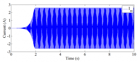
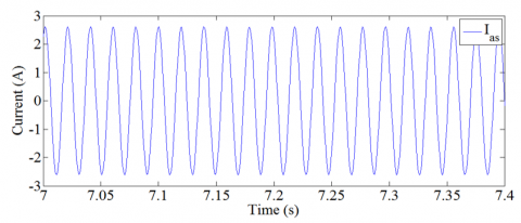
Figure 4 shows the stator current response of the asynchronous no-load generator, one notices that the current response initially takes an increasing form in an exponential way as in the linear case (effect of starting), then converges towards a constant value. Also, the stator current takes a perfectly sinusoidal and balanced form (Figure 5).
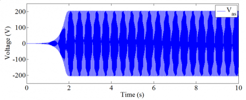
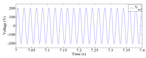
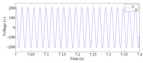
Figure 6 shows the stator voltage response of the asynchronous no-load generator. Initially, the voltage increases exponentially as in the linear case, then it converges towards a constant value depending on the condenser value and the wind speed. Also, one notes that the stator voltage has a sinusoidal form (Figure 7).
Figure 4. Evolution of stator current at no load
Figure 5. Detail of the no-load stator current
Figure 6. No-load stator voltage evolution
Figure 7. Detail of the no-load stator voltage
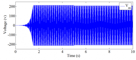
Figure 8 shows the stator voltage curve of an asynchronous generator operating under load at the instant t = 5s. It can be observed that the amplitude of the voltage decreases when the load is applied (Figure 9).
Figure 8. Stator voltage with load
Figure 9. Detail of the stator voltage with load
In this section, we study the use of sliding mode control of an asynchronous cage generator to increase the energy quality. The main purpose of the sliding mode control is to reduce the disturbances and to stabilize the voltage and frequency that the generator produces with different wind intensity values.
To apply the control by sliding mode, oriented flux is required:
\psi_{r d}=\psi_{r} and \psi_{r q}=0 (28)
Then we have:
\frac{d i_{s d}}{d t}=-y_{1} i_{s d}+w_{s} i_{s q}+y_{2} \psi_{r}+\frac{1}{\sigma L_{s}} U_{s d} (29)
\frac{d i_{s q}}{d t}=-w_{s} i_{s d}-y_{3} i_{s q}-w_{s} y_{4} \psi_{r}+\frac{1}{\sigma L_{s}} U_{s q} (30)
\frac{d \psi_{r}}{d t}=\frac{L_{m}}{\tau_{r}} i_{s d}-\frac{1}{\tau_{r}} \psi_{r} (31)
w_{s}=w+\frac{L_{m}}{\tau_{r} \psi_{r}} i_{s q} (32)
with
\tau_{r}: time constant \tau_{r}=\frac{L_{r}}{R_{r}}.
y_{1}=\frac{R_{s}}{\sigma L_{s}}+\frac{L_{m}^{2}}{L_{r} L_{s} \sigma \tau_{r}} (33)
y_{2}=\frac{L_{m}}{L_{r} L_{s} \sigma \tau_{r}} (34)
y_{3}=\frac{R_{s}}{\sigma L_{s}} (35)
y_{4}=\frac{L_{m}}{L_{r} \sigma L_{s}} (36)
3.1 Control design by sliding mode
The implementation of the sliding mode control (SMC) requires three steps [21, 22]:
3.2 Choice of sliding surfaces
We consider the following state model:
[\dot{x}]=[A][x]+[B] \cdot[U] (37)
where, [x] \in R^{n} is the state vector, [U] \in R^{m} is the control vector, with n>m.
Usually, the number of sliding surfaces (SS) chosen is equal to the dimension of the control vector [U].
3.3 The direct switching condition
This is the first condition of convergence. It is proposed and studied by Emelyanov and Utkin. It is about giving the surface a dynamic converging towards zero, and is given in the form [23, 24]:
\dot{s}(x) \cdot s(x)<0 (38)
3.4 Determination of the control law
Once the sliding surface, as well as the convergence criterion are chosen, it remains to determine the control required to attract the variable to be adjusted towards the surface, then towards its point of equilibrium, while maintaining the condition of existence of the sliding mode:
u=u_{e q}+u_{n} (39)
u_{n}=-K \operatorname{sign}(S) (40)
u_{e q} : corresponds to the equivalent command proposed by Filipov and Utkin.
u_{n} : a term introduced to satisfy the following convergence condition:
\dot{S}(x) \cdot S(x)<0 (41)
Therefore, the control law determines the dynamic behavior of the system during the convergence mode. So, this command guarantees the attractiveness of the variable to be checked towards the sliding surface [23, 24].
The outputs to be set are:
y=\left[\psi_{r} U_{d c}\right]^{T} (42)
\left\{\begin{array}{c}S_{1}\left(\psi_{r}\right)=\psi_{r}-\psi_{r}^{{ }^{*}} \\ S_{2}\left(U_{d c}\right)=U_{d c}-U_{d c}{ }^{*} \\ S_{3}\left(i_{s d}\right)=i_{s d}-i_{s d}{ }^{*} \\ S_{4}\left(i_{s q}\right)=i_{s q}-i_{s q}{ }^{*}\end{array}\right. (43)
Then:
i_{s d}^{*}=\frac{\tau_{r}}{L_{m}}\left(\frac{1}{\tau_{r}} \psi_{r}+\dot{\psi}_{r}^{*}\right)-K_{1} \operatorname{sign}\left(s_{1}\right) (44)
i_{s q}=\frac{c U_{d c}}{w \psi_{r}} \frac{L_{r}}{L_{m}}\left(\frac{U_{d c}}{c R}+\dot{U}_{d c}^{*}\right)-K_{2} \operatorname{sign}\left(s_{2}\right) (45)
U_{s d}^{*}=\sigma L_{s}\left(y_{1} i_{s d}-w_{s} i_{s q}-y_{2} \psi_{r}+\dot{I}_{s d}{ }^{*}\right) -K_{3} \operatorname{sign}\left(s_{3}\right) (46)
U_{s q}^{*}=\sigma L_{s}\left(w_{s} i_{s d}+y_{3} i_{s q}+w_{s} y_{4} \psi_{r}+\dot{I}_{s q}{ }^{*}\right)-K_{4} \operatorname{sign}\left(s_{4}\right) (47)
c: DC bus capacitor;
R: line resistance.
The detailed scheme of a sliding mode controller of a self-excited asynchronous generator integrated is illustrated in Figure 10, where the schema presents the control of the system using a sliding mode controller implemented with indirect field orientation control (IFOC) is applied. So, this command is consists of a voltage regulator of the contained bus, current regulators (Isd-Isq) and a block for calculating the angle θS. From the contained bus voltage regulator, we get the reference current Isq, so the current reference Isd is the image of the rotor flux. The reference voltages Vsd and Vsq are the images of the direct and quadrature currents Isd and Isq obtained by a sliding mode controller.
Figure 10. Control diagram by sliding mode applied to the asynchronous cage generator
The sliding mode control applied to the asynchronous cage generator is simulated. Figure 10 shows the control diagram.
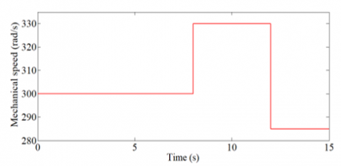
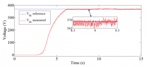
By applying mechanical speed as shown in Figure 11 , and load R_{c h}=1 \Omega and varies at t=10 s to R_{c h}=70 \Omega, we obtain DC bus voltages without and with regulation (Figures 12 and 13).
Figure 11. Wind speed variation
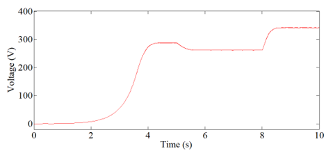
Figure 12. DC bus voltage without regulation
Figure 13. DC bus voltage with regulation using sliding mode regulator
Figure 12 shows the voltage of the DC bus without and with a control respectively. In the first case, the voltage varies with the variation of the wind speed (Figure 11), while in the second one the voltage is well-regulated and follows its reference. One notices that the sliding mode control gives good tracking, no-overshoot, as well as an immediate rejection of wind speed disturbance.
In this work, the modeling and the control of a wind power system based on a self-excited asynchronous generator has been proposed. So, the proposed modeling of self-excited asynchronous generator for the purpose of optimizing the output of a wind turbine. The proposed sliding mode control method by controlling the dc link voltage, which is well known for its robustness, stability, simplicity and very low response time. Indeed, the obtained simulation results confirm that the sliding mode control has shown an improvement in the performance of the mechanical and electrical outputs of a self-excited asynchronous generator.
Authors would like to thank the General Directorate of Scientific Research and Technological Development (DGRSDT) for the support and funding of the research axis through the LEB research laboratory.
|
\Omega_{\text {mec }} |
angular speed of the generator(rad/s) |
|
C_{e m} |
electromagnetic torque (N.m) |
|
V_{s d} and V_{s q} |
stator voltages on the axes (d,q)(V) |
|
\left(i_{s d}\right. and \left.i_{s q}\right) |
stator currents on the axes (d,q)(A) |
|
\left(i_{r d}\right. and \left.i_{r q}\right) |
rotor currents on the axes (d,q)(A) |
|
\left(\psi_{s d}\right. and \left.\psi_{s q}\right) |
stator fluxes on the axes (d,q)(Wb) |
|
\left(\psi_{r d}\right. and \left.\psi_{r q}\right) |
rotor fluxes on the axes (d,q)(Wb) |
|
\mathrm{W}_{\mathrm{sl}}=\mathrm{W}_{\mathrm{s}}-\mathrm{W} |
sliding speed(rad) |
|
\mathrm{W}_{\mathrm{s}} |
rotating field speed(rad/s) |
|
w |
rotor speed(tr/mn) |
|
R_{s} |
stator resistance ( \Omega ) |
|
R_{r} |
rotor resistance ( \Omega ) |
|
\psi_{m} |
magnetizing flux |
|
I_{m} |
magnetizing current |
|
L_{S} |
stator inductance (mH) |
|
L_{r} |
rotor inductance (mH) |
|
L_{m} |
magnetization inductance (mH) |
|
L_{\sigma s} |
stator leakage inductance [mH) |
|
L_{\sigma r} |
rotor leakage inductance (mH) |
|
Greek symbols |
|
|
\rho |
air density (kg/m³) |
|
C_{p} |
power coefficient |
|
S |
surface swept by the blades (m2) |
|
V_{1} |
upstream wind speed (m/s) |
|
r |
blade radius (mm) |
|
G |
gain of the multiplier |
|
J_{T} |
total inertia of rotating parts (kg. m^{-3} ) |
|
f_{T} |
total viscous friction coefficient (N.m.s/rd) |
|
J_{g} |
generator inertia (kg.m2). |
|
\tau_{r} |
time constant |
|
C |
capacitor for excitation (μF) |
|
c |
DC bus capacitor |
|
R |
line resistance |
|
Subscripts |
|
|
MPPT |
Maximum Power Point Tracking |
|
SMC |
Sliding mode control |
|
SS |
Sliding surfaces |
[1] Molinas, M., Suul, J.A., Undeland, T. (2008). Low voltage ride through of wind farms with cage generators: STATCOM versus SVC. IEEE Transactions on Power Electronics, 23(3): 1104-1117. https://doi.org/10.1109/TPEL.2008.921169
[2] Chen, Z., Guerrero, J.M., Blaabjerg, F. (2009). A review of the state of the art of power electronics for wind turbines. IEEE Transactions on Power Electronics, 24(8): 1859-1875. https://doi.org/10.1109/TPEL.2009.2017082
[3] Lei, Y., Mullane, A., Lightbody, G., Yacamini, R. (2006). Modeling of the wind turbine with a doubly fed induction generator for grid integration studies. IEEE Transactions on Energy Conversion, 21(1): 257-264. https://doi.org/10.1109/TEC.2005.847958
[4] Tabak, N.A. (2020). Modeling, vector control and simulation of wind turbine with dual excited synchronous generator. Tishreen University Journal for Research and Scientific Studies - Engineering Sciences Series, 42(4). Available from: http://journal.tishreen.edu.sy/index.php/engscnc/article/view/9908.
[5] Suarez, E., Bortolotto, G. (1999). Voltage-frequency control of a self-excited induction generator. IEEE Transactions on Energy Conversion, 14(3): 394-401. https://doi.org/10.1109/60.790888
[6] Chen, W.L., Hsu, Y.Y. (2006). Controller design for an induction generator driven by a variable-speed wind turbine. IEEE Transactions on Energy Conversion, 21(3): 625-635. https://doi.org/10.1109/TEC.2006.875478
[7] Palle, B., Simões, M.G., Farret, F.A. (2005). Dynamic simulation and analysis of parallel self-excited induction generators for islanded wind farm systems. IEEE Transactions on Industry Applications, 41(4): 1099-1106. https://doi.org/10.1109/TIA.2005.851040
[8] Chan, T.F. (1993). Capacitance requirements of self-excited induction generators. IEEE Transactions on Energy Conversion, 8(2): 304-311. https://doi.org/10.1109/60.222721
[9] Abdin, E.S., Xu, W. (2000). Control design and dynamic performance analysis of a wind turbine-induction generator unit. IEEE Transactions on Energy Conversion, 15(1): 91-96. https://doi.org/10.1109/60.849122
[10] Palle, B., Simões, M.G., Farret, F.A. (2005). Dynamic simulation and analysis of parallel self-excited induction generators for islanded wind farm systems. IEEE Transactions on Industry Applications, 41(4): 1099-1106. https://doi.org/10.1109/TIA.2005.851040
[11] Zaidi, E., Marouani, K., Bouadi, H., Nounou, K., Aissani, M., Bentouhami, L. (2019). Control of a multiphase machine fed by multilevel inverter based on sliding mode controller. In 2019 IEEE International Conference on Environment and Electrical Engineering and 2019 IEEE Industrial and Commercial Power Systems Europe (EEEIC/I&CPS Europe), pp. 1-6. https://doi.org/10.1109/EEEIC.2019. 8783559
[12] Yang, X., Liu, G., Li, A., Le, V.D. (2017). Predictive power control strategy for ds based on a wind energy converter system. Energies, 10(8): 2-24. https://doi.org/10.3390/en10081098
[13] Boldea, I. (2006). Variable Speed Generators. Taylor & Francis, USA. ISBN 9781498723572.
[14] Leonhard, W. (2001). Control of Electrical Drives. Berlin, Germany: Springer-Verlag. Third edition, ISBN 3-5440-41820-2.
[15] García, G.O., Luis, J.C.M., Stephan, R.M., Watanabe, E.H. (1994). An efficient controller for an adjustable speed induction motor drive. IEEE Transactions on Industrial Electronics, 41(5): 533-539. https://doi.org/10.1109/ 41.315272
[16] Ahmed, T., Nishida, K., Nakaoka, M. (2006). Advanced control of PWM converter with variable-speed induction generator. IEEE Transactions on Industry Applications, 42(4): 934-945. https://doi.org/10.1109/TIA.2006.876068
[17] Leidhold, R., Garcia, G., Valla, M.I. (2002). Field-oriented controlled induction generator with loss minimization. IEEE Transactions on Industrial Electronics, 49(1): 147-156. https://doi.org/10.1109/41.982258
[18] Harrington, R.J., Bassiouny, F.M.M. (1998). New approach to determine the critical capacitance for self-excited induction generators. IEEE Transactions on Energy Conversion, 13(3): 244-249. https://doi.org/10.1109/60.707603
[19] Benchagra, M., Hilal, M., Errami, Y., Ouassaid, M., Maaroufi, M. (2011). Modeling and control of SCIG based variable-speed with power factor control. International Review on Modelling and Simulations (IREMOS), 4(3): 1007-1014.
[20] Senjyu, T., Ochi, Y., Kikunaga, Y., Tokudome, M., Yona, A., Muhando, E.B., Funabashi, T. (2009). Sensor-less maximum power point tracking control for wind generation system with squirrel cage induction generator. Renewable Energy, 34(4): 994-999. https://doi.org/10.1016/j.renene.2008.08.007
[21] Cupertino, F., Naso, D., Mininno, E., Turchiano, B. (2009). Sliding-mode control with double boundary layer for robust compensation of payload mass and friction in linear motors. IEEE Transactions on Industry Applications, 45(5): 1688-1696. https://doi.org/10.1109/TIA.2009.2027521
[22] Kim, Y.K., Jeon, G.J. (2004). Error reduction of sliding mode control using sigmoid-type nonlinear interpolation in the boundary layer. International Journal of Control, Automation, and Systems, 2(4): 523-529.
[23] Kung, C.C., Su, K.H. (2005). Adaptive fuzzy position control for electrical servodrive via total-sliding-mode technique. IEE Proceedings-Electric Power Applications, 152(6): 1489-1502. https://doi.org/10.1049/ip-epa:20045253
[24] Wai, R.J., Su, K.H. (2006). Adaptive enhanced fuzzy sliding-mode control for electrical servo drive. IEEE Transactions on Industrial Electronics, 53(2): 569-580. https://doi.org/10.1109/TIE.2006.870710