Uma Ravi Sankar Yalavarthy* | Venkata Siva Krishna Rao Gadi
© 2022 IIETA. This article is published by IIETA and is licensed under the CC BY 4.0 license (http://creativecommons.org/licenses/by/4.0/).
OPEN ACCESS
This paper presents a high performance squirrel-cage asynchronous motor (ASM) drive, proposed for high-speed electric vehicle (EV) propulsion. This is an indirect space vector control (IDSVC) scheme in the rotor flux frame of reference, in which the modeling is based on synchronously rotating coordinate system transformation. Space vector pulse width modulation (SVPWM) inverter fetches the controlled stator direct and quadrature axis responses from the speed and current controllers and supply necessary voltages to stator of ASM. The output voltage waveforms of SVPWM inverter are not sinusoidal in nature, which allows undesired harmonics at high frequency of operation. This due to inconsistent switching frequency. A second-order low-pass (SOLP) RLC filter with Butterworth approximation and was designed and connected in series with SVPWM inverter to grab harmonic free speed and torque profile during high speed operations. Similarly, another SOLP with a quality factor equal to 2 is designed and speed profiles of both filters are compared. The system is developed and simulated in MATLAB/SIMULINK to observe the speed and torque tracking capabilities. Simulation results show that the performance of drive under steady and dynamic states were good with Butterworth filter approximation with robust IDSVC scheme adopted over wide range speed-drive curve.
asynchronous motor (ASM), electric vehicle (EV), indirect space vector control (IDSVC), second-order low-pass (SOLP), space vector pulse width modulation (SVPWM)
Vehicle propulsion system now-a -days mainly concern to the eco-friendly and green transportation. The depletion of fossil fuels, carbon dioxide (CO2) emission and ever- growing energy demand are the leading contributors of climatic change and environmental pollution [1], which paid attention to the EV. EV’s are the promising technology for the energy efficient and pollution free environment compared to internal combustion engine vehicle (ICEV) [2, 3].
Advances in power converter design for renewable energy sources and charging electric vehicles made EV’s more reliable [4]. In EV’s, numerous types of machines are employed, out of them synchronous motors with permanent magnet (PMSM) and ASMs are used for propelling. ASM is widely preferred because it gives best compliance in manufacturing cost and power density. It is also simple in construction, high reliable, minimum torque ripple, easy in control, low noise and a robust machine. Moreover, it is highly efficient at medium and high frequencies with minimum iron losses [5, 6]. The control schemes mainly applied to ASM are V/F control, adaptive control, direct torque control and fuzzy logic control [7-10]. The IDSVC of ASM is the basic closed loop control scheme with less complexity in design and operation and could achieve the requirements of high-performance speed regulation.
In this paper, the indirect space vector control scheme implementation for asynchronous motor involves the conversion of the actual stator and rotor three phase windings by an equivalent set of orthogonal di-phasic windings and further to d-q orthogonal windings, which produces same MMF in the air gap, without direct consideration of Park’s transformation matrix [11]. Nevertheless, transformation matrix is derived by physical approach. The indirect space vector control strategy for torque and speed regulation is exercised and then finally the SVPWM inverter in association with SOLP RLC filter with Butterworth approximation is employed to achieve harmonic free speed and torque curve in high speed traction.
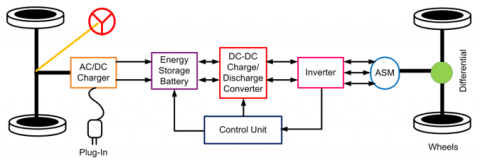
The architecture of battery powered plug-in EV is shown in Figure 1. The pure electric vehicle basically constitutes of an asynchronous motor, inverter, charge/discharge DC-DC converter, battery for energy storage, control unit and plug-in electric charger [12]. The double line represents the DC supply connections and triple line the represents three phase supply connections. The bidirectional arrows represent the power flow in either direction. The battery is charged with a plug-in electric charger. The control unit gives the necessary commands to DC-DC converter and battery, which enables the charging or discharging modes of battery. To achieve motoring of EV either during acceleration or constant speed operations, the power flow is from battery to inverter and then to electric motor. The type of braking adopted in an EV is the regenerative braking. During deceleration of EV, the power flows in counter direction to charge the battery.
The DC-DC charge/discharge converter in association with control unit takes care of voltage diverseness during motoring and braking operations. Unlike internal combustion vehicles, EV’s are more flexible in operation and maintenance as they are more advanced in transmission and conversion of energy.
Figure 1. Electric vehicle architecture
The DC-DC charge/discharge converter in association with control unit takes care of voltage diverseness during motoring and braking operations. Unlike internal combustion vehicles, EV’s are more flexible in operation and maintenance as they are more advanced in transmission and conversion of energy.
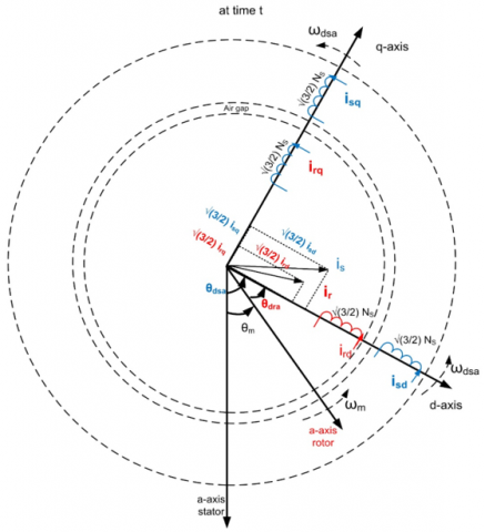
For dynamic analysis of ASM, we need two orthogonal windings by which the flux and torque can alone be governed. The stator and rotor have equal number of turns (Ns). Assume the stator windings be wye-connected where neutral not accessible and the number of turns of orthogonal windings as $\sqrt{3 / 2}$Ns such that d-q windings have same stator resistance and leakage reactance similar to three phase windings.
Figure 2. d-q winding representation of stator and rotor currents
$\overrightarrow{u_{s}^{a}}(t)=u_{a}(t) e^{j 0}+u_{b}(t) e^{\frac{j 2 \pi}{3}}+u_{c}(t) e^{\frac{j 4 \pi}{3}}=u^{\wedge}(t) e^{j \theta_{u_{s}}(t)}$ (1)
$\overrightarrow{i_{s}^{a}}(t)=i_{a}(t) e^{j 0}+i_{b}(t) e^{\frac{j 2 \pi}{3}}+i_{c}(t) e^{\frac{j 4 \pi}{3}}=i^{\wedge}(t) e^{j \theta_{i_{s}}(t)}$ (2)
$\overrightarrow{\psi_{s}^{a}}(t)=\psi_{a}(t) e^{j 0}+\psi_{b}(t) e^{\frac{j 2 \pi}{3}}+\psi_{c}(t) e^{\frac{j 4 \pi}{3}}=\psi^{\wedge}(t) e^{j \theta_{\psi_{s}}(t)}$ (3)
where, $\overrightarrow{u_{s}^{a}}(t), \overrightarrow{i_{s}^{d}}(t)$ and $\overrightarrow{\psi_{s}^{a}}(t)$ are stator three phase space vectors and $u^{\wedge}(t) e^{j \theta_{u_{s}}(t)}, i^{\wedge}(t) e^{j \theta_{i_{s}}(t)}$ and $\psi^{\wedge}(t) e^{j \theta_{\psi_{s}}(t)}$ are stator three phase phasors referred to stator a-axis. The MMF distribution produced by the hypothetical d-q winding in the air gap is same, similar to three phase stator windings [Appendix 1]. The stator current space vector with reference d-axis is given in Eq. (4), (5) [13].
$\overrightarrow{l_{s}^{d}}(t)=i_{a}(t) e^{-j \theta_{d s a}+i_{b}}(t) e^{-j\left(\theta_{d s a}-\frac{2 \pi}{3}\right)}+i_{c}(t) e^{-j\left(\theta_{d s a}-\frac{4 \pi}{3}\right)}$ (4)
$\overrightarrow{i_{s}^{d}}(t)=\sqrt{\frac{3}{2}}\left(i_{s d}(t)+j i_{s q}(t)\right)$ (5)
From Figure 2 it is observed
$i_{s d}(t)=\sqrt{\frac{2}{3}}\left(\right.$ Projection of $i_{s}(t)$ along $d$-axis $)$
$=\sqrt{\frac{2}{3}} \cdot\left(\frac{3}{2} \hat{i}_{\mathrm{s}}\right) \cos \theta_{\mathrm{dsa}}$ (6)
$\mathrm{i}_{\mathrm{sq}}(\mathrm{t})=\sqrt{\frac{2}{3}}\left(\right.$ Projection of $\mathrm{i}_{\mathrm{s}}(\mathrm{t})$ along $\mathrm{q}$-axis $)$
$=\sqrt{\frac{2}{3}} \cdot\left(\frac{3}{2} \hat{\mathrm{i}}_{\mathrm{s}}\right) \sin \theta_{\mathrm{dsa}}$ (7)
Equating the real and imaginary parts of Eq. (4) and Eq. (5). In the situation of an isolated neutral, the sum of all 3-phase currents is always zero. The dq0 winding variables can be determined in terms of abc winding variables. The bottom third row of ones in the matrix shows the situation where the total of all 3-phase currents is zero, $i_{s 0}(t)=i_{a}(t)+i_{b}(t)+i_{c}(t)=0$. Therefore, we omit the third row and consider a 2x3 matrix instead of 3x3 matrix as shown in Eq. (8.2).
$\left(\begin{array}{c}i_{s d}(t) \\ i_{s q}(t) \\ i_{s 0}(t)\end{array}\right)=$
$\sqrt{\frac{2}{3}}\left(\begin{array}{ccc}\cos \left(\theta_{d s a}\right) & \cos \left(\theta_{d s a^{-}} \frac{2 \pi}{3}\right) & \cos \left(\theta_{d s a^{-}} \frac{4 \pi}{3}\right) \\ -\sin \left(\theta_{d s a}\right) & -\sin \left(\theta_{d s a^{-}} \frac{2 \pi}{3}\right) & -\sin \left(\theta_{d s a^{-}} \frac{4 \pi}{3}\right) \\ 1 & 1 & 1\end{array}\right)$
$\left(\begin{array}{l}i_{a}(t) \\ i_{b}(t) \\ i_{c}(t)\end{array}\right)$ (8.1)
$\left(\begin{array}{l}i_{s d}(t) \\ i_{s q}(t)\end{array}\right)=$
$\sqrt{\frac{2}{3}}\left(\begin{array}{ccc}\cos \left(\theta_{d s a}\right) & \cos \left(\theta_{d s a^{-}} \frac{2 \pi}{3}\right) & \cos \left(\theta_{d s a^{-}} \frac{4 \pi}{3}\right) \\ -\sin \left(\theta_{d s a}\right) & -\sin \left(\theta_{d s a^{-}} \frac{2 \pi}{3}\right) & -\sin \left(\theta_{d s a^{-}} \frac{4 \pi}{3}\right)\end{array}\right)$
$\left(\begin{array}{l}i_{a}(t) \\ i_{b}(t) \\ i_{c}(t)\end{array}\right)$ (8.2)
The 2×3 matrix is called state transformation matrix [Zs]abc-dq0 given in Eq. (8.2). Similarly, we apply the same transformation matrix for stator voltages and flux linkages. Consider Eq. (8.1) and solve for abc phase currents in terms of dq0 winding currents. The inverse 3x3 matrix in Eq. (8.1) is given in Eq. (9.1). We get the necessary relationship by removing the third column of ones which has no contribution as shown in Eq. (9.2).
$\left(\begin{array}{l}i_{a}(t) \\ i_{b}(t) \\ i_{c}(t)\end{array}\right)=\sqrt{\frac{2}{3}}\left(\begin{array}{ccc}\cos \left(\theta_{d s a}\right) & -\sin \left(\theta_{d s a}\right) & 1 \\ \cos \left(\theta_{d s a}+\frac{4 \pi}{3}\right) & -\sin \left(\theta_{d s a}+\frac{4 \pi}{3}\right) & 1 \\ \cos \left(\theta_{d s a}+\frac{2 \pi}{3}\right) & -\sin \left(\theta_{d s a}+\frac{2 \pi}{3}\right) & 1\end{array}\right)$
$\left(\begin{array}{c}i_{s d}(t) \\ i_{s q}(t) \\ i_{s 0}(t)\end{array}\right)$ (9.1)
$\left(\begin{array}{c}i_{a}(t) \\ i_{b}(t) \\ i_{c}(t)\end{array}\right)=\sqrt{\frac{2}{3}}\left(\begin{array}{cc}\cos \left(\theta_{d s a}\right) & -\sin \left(\theta_{d s a}\right) \\ \cos \left(\theta_{d s a}+\frac{4 \pi}{3}\right) & -\sin \left(\theta_{d s a}+\frac{4 \pi}{3}\right) \\ \cos \left(\theta_{d s a}+\frac{2 \pi}{3}\right) & -\sin \left(\theta_{d s a}+\frac{2 \pi}{3}\right)\end{array}\right)$
$\left(\begin{array}{l}i_{s d}(t) \\ i_{s q}(t)\end{array}\right)$ (9.2)
Here, the 3×2 matrix is also called state transformation matrix [Zs]dq-abc in reverse direction. The same procedure is adopted to derive the rotor d-q quantities, assuming the rotor is wound with three phase winding similar to stator three phase winding and replacing θdsa with θdra. To derive the Stator winding equations, consider a pair of orthogonal α-β windings lined up to stator which is shown in Figure 3. That is α-axis lined up to stator a-axis. Similarly, we can derive rotor winding equations by considering Figure 4.
Figure 3. α-β and d-q equivalent windings of stator
Figure 4. α-β and d-q equivalent windings of rotor
usα = Rsisα + $\frac{d}{d t} \psi$sα (10)
usβ = Rsisβ + $\frac{d}{d t} \psi$sβ (11)
Since α and β components are orthogonal combine Eq. (10) and Eq. (11) with j operator for space vector representation.
$\overrightarrow{u_{s_{-} \alpha \beta}^{\alpha}}=R_{s} \overrightarrow{i_{s_{-} \alpha \beta}^{\alpha}}+\frac{d}{d t} \overrightarrow{\psi_{s \alpha \beta}^{\alpha}}$ (12)
where, $\overrightarrow{u_{s_{-} \alpha \beta}^{\alpha}}$ =uα+juβ.
The α-axis reference orthogonal α and β space vector components can be related to d-axis reference orthogonal d-q components. The function of this representation is to convert orthogonal α- β components in stationary frame of reference into d-q components in rotating frame of reference. This is how the Park’s transformation can be achieved.
$\overrightarrow{u_{s \quad \alpha \beta}^{\alpha }}=\overrightarrow{u_{s \quad d q}^{\alpha} } e^{j \theta_{d s a}}$ (13)
$\overrightarrow{i_{s \quad \alpha \beta}^{\alpha }}=\overrightarrow{i_{s \quad d q}^{\alpha} } e^{j \theta_{d s a}}$ (14)
Substituting Eq. (13), (14) in Eq. (12),
$\overrightarrow{u_{s_{-} d q}^{\alpha}}$ = Rs $\overrightarrow{i_{s_{d q}}^{\alpha} }$ + $\frac{d}{d t} \overrightarrow{\psi_{s \quad d q }^{\alpha}}$ +jωd $\overrightarrow{\psi_{s\quad {d q}}^{\alpha} }$ (15)
where, $\frac{\mathrm{d}}{\mathrm{dt}}$θdsa= ωdsa, instantaneous speed (rad.s-1).
usd = Rsisd + $\frac{d}{d t} \psi$sd - ψsqωdsa (16)
usq = Rsisq +$\frac{d}{d t} \psi$ sq + ψsdωdsa (17)
$\left[\begin{array}{l}u_{s d} \\ u_{s q}\end{array}\right]=R_{s}\left[\begin{array}{l}i_{s d} \\ i_{s q}\end{array}\right]+\frac{d}{d t}\left[\begin{array}{l}\psi_{s d} \\ \psi_{s q}\end{array}\right]+\omega_{d s a}\left[\begin{array}{cc}0 & -1 \\ 1 & 0\end{array}\right]\left[\begin{array}{l}\psi_{s d} \\ \psi_{s q}\end{array}\right]$ (18)
To obtain the rotor equations, we assume the rotor was wound with 3-phase windings and follow the same approach as was used to obtain the stator windings earlier. Simply replace the suffix s (stator) with r (rotor) and dsa with dra in Eq. (18) instead of going through the overall process.
$\left[\begin{array}{l}u_{r d} \\ u_{r q}\end{array}\right]=R_{r}\left[\begin{array}{l}i_{r d} \\ i_{r q}\end{array}\right]+\frac{d}{d t}\left[\begin{array}{l}\psi_{r d} \\ \psi_{r q}\end{array}\right]+\omega_{d r a}\left[\begin{array}{cc}0 & -1 \\ 1 & 0\end{array}\right]\left[\begin{array}{l}\psi_{r d} \\ \psi_{r q}\end{array}\right]$ (19)
Note that for squirrel cage rotor with short circuited rotor bars $\left[\begin{array}{l}u_{r d} \\ u_{r q}\end{array}\right]=\left[\begin{array}{l}0 \\ 0\end{array}\right]$. Flux linkages in terms of input voltages and currents are obtained from Eq. (18), (19).
$\frac{d}{d t}\left[\begin{array}{l}\psi_{s d} \\ \psi_{s q}\end{array}\right]=\left[\begin{array}{l}u_{s d} \\ u_{s q}\end{array}\right]-R_{s}\left[\begin{array}{l}i_{s d} \\ i_{s q}\end{array}\right]-\omega_{d s a}\left[\begin{array}{cc}0 & -1 \\ 1 & 0\end{array}\right]\left[\begin{array}{l}\psi_{s d} \\ \psi_{s q}\end{array}\right]$ (20)
$\frac{d}{d t}\left[\begin{array}{l}\psi_{r d} \\ \psi_{r q}\end{array}\right]=\left[\begin{array}{l}u_{r d} \\ u_{r q}\end{array}\right]-R_{r}\left[\begin{array}{l}i_{r d} \\ i_{r q}\end{array}\right]-\omega_{d r a}\left[\begin{array}{cc}0 & -1 \\ 1 & 0\end{array}\right]\left[\begin{array}{l}\psi_{s d} \\ \psi_{s q}\end{array}\right]$ (21)
Eq. (20), (21) can be rewritten as
$\frac{d}{d t}\left[\overrightarrow{\psi_{s_{-} d q}}\right]=\left[u_{s_{-}} d q\right]-R_{s}\left[i_{s_{-} d q}\right]-\omega_{d s a}\left[A_{\text {rotate }}\right]\left[\psi_{s_{-} d q}\right]$ (22)
$\frac{d}{d t}\left[\overrightarrow{\psi_{r_{-} d q}}\right]=\left[u_{r_{-} d q}\right]-R_{r}\left[i_{r_{-}} d q\right]-\omega_{\text {dra }}\left[A_{\text {rotate }}\right]\left[\psi_{r_{-} d q}\right]$ (23)
Space vector $\overrightarrow{\psi_{s_{-} d q}}$ is rotated by an angle of π/2 with the matrix $\left[A_{\text {rotate }}\right]$ =$\left[\begin{array}{cc}0 & -1 \\ 1 & 0\end{array}\right]$. On rotor d-axis and q-axis winding, electromagnetic torque is given in Eq. (24), (25) [13].
$T_{d(\text { rotor })}=\frac{p}{2}\left(L_{m} i_{s q}+L_{r} i_{r q}\right) i_{r q}=\frac{p}{2}\left(\psi_{r q}\right) i_{r d}$ (24)
$T_{q(\text { rotor })}=-\frac{p}{2}\left(L_{m} i_{s d}+L_{r} i_{r d}\right)=-\frac{p}{2}\left(\psi_{r d}\right) i_{r q}$ (25)
The constraints for the establishment of flux linkages are (1) The d-axis windings and q-axis windings have zero mutual coupling. (2) The flux that links any winding is caused by its self current as well as the current of the other winding on the same axis. One could write flux expressions for all four windings using this logic. The flux linkages in terms of their direct and quadrature currents in stator and rotor are given in Eq. (26), (27), (28) and (29).
$\psi_{s d}=L_{s} i_{s d}+L_{m} i_{r d}$ (26)
$\psi_{s q}=L_{s} i_{s q}+L_{m} i_{r q}$ (27)
$\psi_{r d}=L_{r} i_{r d}+L_{m} i_{s d}$ (28)
$\psi_{r q}=L_{r} i_{r q}+L_{m} i_{s q}$ (29)
where, Rs and Rr are per phase stator and rotor resistances in ohm respectively. Ls, Lr and Lm are per phase stator, rotor and magnetizing inductances in Henry respectively. Total electromagnetic torque $T_{E}=T_{d(\text { rotor })}+T_{q \text { (rotor })}$ (N-m).
$T_{E}=\frac{p}{2}\left(\psi_{r q} i_{r d}-\psi_{r d} i_{r q}\right)$ (30)
$T_{E}=\frac{p}{2} L_{m}\left(i_{s q} i_{r d}-i_{s d} i_{r q}\right)$ (31)
$\omega_{M e c h}=\frac{2}{p}\left(\omega_{m}\right)$ (32)
$\frac{d}{d t} \omega_{M e c h}=\frac{\left(T_{E^{-}} T_{L}\right)}{J}$ (33)
where, $\omega_{M e c h}$ is mechanical speed of motor (rad-s-1), TL is the load torque (N-m), Representing the Eq. (26, 27, 28, 29) in matrix form. Let the M stands for 4x4 matrix [Appendix 2].
$\left[\begin{array}{l}\psi_{s d} \\ \psi_{s q} \\ \psi_{r d} \\ \psi_{r q}\end{array}\right]=\left[\begin{array}{cccc}L_{s} & 0 & L_{m} & 0 \\ 0 & L_{s} & 0 & L_{m} \\ L_{m} & 0 & L_{r} & 0 \\ 0 & L_{m} & 0 & L_{r}\end{array}\right]\left[\begin{array}{l}i_{s d} \\ i_{s q} \\ i_{r d} \\ i_{r q}\end{array}\right]$ (34)
$\left[\begin{array}{llll}i_{s d} & i_{s q} & i_{r d} & i_{r q}\end{array}\right]^{T}=M^{-1}\left[\begin{array}{llll}\psi_{s d} & \psi_{s q} & \psi_{r d} & \psi_{r q}\end{array}\right]^{T}$ (35)
In Figure 2 each alone stator and rotor d-axis windings are aligned to rotor flux ($\overrightarrow{\psi_{r}}$) to draw simplified equations. We will represent $\boldsymbol{\omega}_{d r a}$ and electromagnetic torque in terms of $i_{s q}$ and $\psi_{r d}$. Under vector-controlled operation, $\psi_{r d}$ is kept invariable and $i_{s q}$ steer the electromagnetic torque generation. The dynamics for $\psi_{r d}$ are built. In the alignment of d-axis of both stator and rotor to rotor flux ($\overrightarrow{\psi_{r}}$), which that means that the q-axis of both stator and rotor windings will be orthogonal to the rotor flux. So, q-axis rotor winding will not have any flux linking with the rotor flux. Hence q-axis rotor flux linkages are zero as given in Eq. (36). The absence of q- axis rotor flux linkages indicates that the rate of change of their flux linkage will definitely be equals to zero.
$\psi_{r q}=0, \Rightarrow \frac{d}{d t}\left(\psi_{r q}\right)=0$ (36)
For a squirrel cage rotor $\left[\begin{array}{l}u_{r d} \\ u_{r q}\end{array}\right]=\left[\begin{array}{l}0 \\ 0\end{array}\right]$ (37)
Substituting Eq. (36) in Eq. (29).
$i_{r q}=-\left(\frac{L_{m}}{L_{r}}\right) i_{s q}$ (38)
On substitution of Eq. (36), (37) in Eq. (19) for $\mathrm{\omega}_{d r a}$.
$\omega_{d r a}=-R_{r}\left(\frac{i_{r q}}{\psi_{r d}}\right)$ (39)
Let rotor time constant from Figure $5, \tau_{r}=\left(\frac{L_{r}}{R_{r}}\right)$ (40)
Substituting Eq. (38), (40) in Eq. (39).
$\omega_{d r a}=\left(\frac{L_{m}}{\tau_{r} \psi_{r d}}\right) i_{s q}$ (41)
Then substituting Eq. (36) in Eq. (30) for $T_{E}$.
$T_{E}=-\frac{p}{2}\left(\psi_{r d} i_{r q}\right)$ (42)
Substitute Eq. (38) in Eq. (42),
$T_{E}=\frac{p}{2} \psi_{r d}\left(\frac{L_{m}}{L_{r}} i_{s q}\right)$ (43)
Figure 5. A simplified d-axis circuitry with current excitation
Figure 5 is the d-axis circuit for short-circuited squirrel cage rotor with current excitation. Where $L_{l r}$ is per phase rotor leakage inductance and $L_{r}=L_{l r}+L_{m}$. Solve the circuit for $i_{r d}$ in Laplace domain.
$i_{r d}(s)=-\frac{s L_{m}}{\left(R_{r}+s L_{r}\right)} i_{s d}(s)$ (44)
Substituting Eq. (44) in Eq. (28) and using Eq. (40)
$\psi_{r d}(s)=\frac{L_{m}}{\left(1+s \tau_{r}\right)} i_{s d}(s)$ (45)
Figure 6 presents the block diagram of actual ASM, which was developed employing Eq. (41), (43, (45). Here stator direct and quadrature currents along with mechanical speed of rotation are given as input and electromagnetic torque, d-axis rotor flux linkages and rotor position are output quantities. Where $\omega_{d s a}$ is the instantaneous speed of stator d-q winding pair with reference to stator a-axis and $\omega_{d s a}=\omega_{d r a}+\omega_{m}$. The Simulink model ASM corresponding to Figure 6 is shown in Figure 7.
In Figure 8, utilizing the computed values of $i_{s d}, i_{s q}$ and $\psi_{r d}$ for an any value of $\omega_{d s a}$ measured, the reference voltages $u_{s d}^{r e f}$ and $u_{s q}^{r e f}$ are generated. The direct and quadrature stator voltages with the estimated value of $\theta_{d s a}$ undergo dq to abc transformation and reference voltage signals $u_{a}^{r e f}, u_{b}^{r e f}$ and $u_{c}^{r e f}$ are produced. The reference voltage signals are fed to SVPWM converter to the operating three phase voltages $u_{a}, u_{b}$ and $u_{c}$ to ASM to acquire desired operation. The three phase stator currents of actual motor undergo abc to dq and are driven to estimated motor model to achieve the estimated values of torque $T_{E \text { (est) }}$, $\psi_{r d \text { (est) }}$ and $\theta_{d s a(\text { est })}$. The direct and quadrature stator currents of actual motor model are compared with their corresponding reference values to generate an error signal. Each alone d-axis and q-axis error signals are given respective PI torque controllers as shown in Figure 9. To design PI torque controller the following procedure is implemented.
Figure 6. Actual ASM model d-axis oriented with ($\overrightarrow{\psi_{r}}$)
Figure 7. Simulink model of actual ASM
Figure 8. A block diagram of indirect space vector control of ASM accompanied by applied voltages
Firstly, we have to compute the required reference stator voltages that SVPWM power processing unit that have to supply ASM as shown in Figure 8. Let leakage factor (σ) of ASM is given in Eq. (46) [13].
$\sigma=\frac{L_{s} L_{r}-L_{s}^{2}}{L_{s} L_{r}}$ (46)
Solve for $i_{r d}$ in Eq. (28) and then substituting in Eq. (26).
$\psi_{s d}=\sigma L_{s} i_{s d}+\frac{L_{m}}{L_{r}} \psi_{r d}$ (47)
Substituting Eq. (38) in Eq. (27) for $\psi_{s q}$.
$\psi_{s q}=\sigma L_{s} i_{s q}$ (48)
Substituting Eq. (46), (47) in Eq. (16), (17) respectively.
$u_{s d}=\left(R_{s} i_{s d}+\sigma L_{s} \frac{d}{d t} i_{s d}\right)+\left(\frac{L_{m}}{L_{r}} \frac{d}{d t} \psi_{r d}-\omega_{d s a} \sigma L_{s} i_{s q}\right)$ (49)
$u_{s q}=\left(R_{s} i_{s q}+\sigma L_{s} \frac{d}{d t} i_{s q}\right)+\left(\omega_{d s a} \frac{L_{m}}{L_{r}} \frac{d}{d t} \psi_{r d}+\omega_{d s a} \sigma L_{s} i_{s d}\right)$ (50)
In Eq. (49) for d-axis stator voltage, on RHS only the initial two terms in the first set of brackets rely on d-axis stator current, while the other two terms are treated as disturbances and can be ignored. Similarly, disturbances for q-axis stator voltage in Eq. (50) are omitted. The error caused by the disturbances in stator d-axis and q-axis voltages is only about two to three percent of the sum of initial two terms in the first set of brackets in Eq. (49) and Eq. (50) respectively. These disturbance terms are treated as compensated terms. They could be compensated by considering these compensation terms. In this analysis, they have been ignored.
$u_{s d}^{\prime}=\left(R_{s} i_{s d}+\sigma L_{s} \frac{d}{d t} i_{s d}\right)$ (51)
$u_{s q}^{\prime}=\left(R_{s} i_{s q}+\sigma L_{s} \frac{d}{d t} i_{s q}\right)$ (52)
Applying Laplace transformation to Eq. (51), (52).
$u_{s d}^{\prime}(s)=\left(R_{s}+s \sigma L_{s}\right) i_{s d}(s)$ (53)
$u_{s q}^{\prime}(s)=\left(R_{s}+s \sigma L_{s}\right) i_{s q}(s)$ (54)
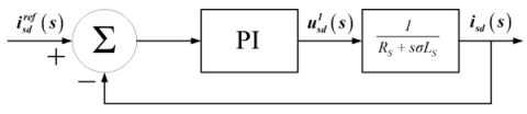
Figure 9 show the block diagram current control loop on d-axis winding, designed from Eq. (53). Similarly speed control loop on q-axis winding is designed from Eq. (54).
Figure 9. A d-axis current control loop schematic
In steady state under vector control $\psi_{r d}$ is constant, which implies $\frac{d \psi_{r d}}{d t}=0$, from Eq. (36), $\psi_{r q}=0$, $\frac{d \psi_{r q}}{d t^{2}}=0$, and for squirrel-cage rotor $u_{r d}=0$. Substituting above values in Eq. (19).
$i_{r d}=0$ (55)
On substitution of Eq. (55) in Eq. (28)
$\psi_{r d}=L_{m} i_{s d}$ (56)
On substitution of Eq. (56) in Eq. (43)
$T_{E}=\frac{p}{2}\left(\frac{L_{m}^{2}}{L_{r}}\right) i_{s d}{ }^{r e f} i_{s q}$ (57)
where, $K_{T}=\frac{p}{2}\left(\frac{L_{m}^{2}}{L_{r}}\right) i_{s d}{ }^{r e f}$ (58)
$\omega_{M e c h}=\frac{1}{J} \int\left(T_{E}-T_{L}\right)$ (59)
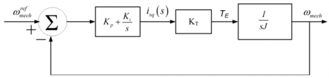
Figure 10. A speed loop controller schematic
Figure 10 is the block diagram of speed control loop, where $\omega_{M e c h}^{r e f}$cc is reference speed and $\omega_{M e c h}$ actual mechanical speed of ASM. The error in the position is fed to PI controller. The proportionality constants for current and speed loop controllers for particular values of crossover frequency and phase margin are derived. In the control scheme of ASM, at initial start-up before zero speed the electromagnetic torque is zero, where $\psi_{r d}$ builds up to its rated value which is dependent on $i_{s d}$ evident from Eq. (56). Once the core gets full magnetized, $\psi_{r d}$ remain unchanged and then the torque varies according to $i_{s q}$ from Eq. (57). There after the drive follows the speed, torque and position commands.
The SVPWM scheme is used mostly in vector controlled drives. Space vector stator voltage in terms of instantaneous phase voltages of stator can be represented in Eq. (60) [13]. The stator winding is star connected, assume hypothetically neutral of stator and negative of DC as reference ground as shown in Figure 11.
$\overrightarrow{u_{s}^{a}(t)}=u_{a}(t) e^{j 0}+u_{b}(t) e^{\frac{j 2 \pi}{3}}+u_{c}(t) e^{\frac{j 4 \pi}{3}}$ (60)
$u_{a}=u_{a n}+u_{n}, u_{b}=u_{b n}+u_{n}, u_{c}=u_{c n}+u_{n}$ (61)
Figure 11. A switching power inverter (PPU)
On Substitution of Eq. (61) in Eq. (60)
$\overrightarrow{u_{s}^{a}}(t)=u_{a n}(t) e^{j 0}+u_{b n}(t) e^{\frac{j 2 \pi}{3}}+u_{c n}(t) e^{\frac{j 4 \pi}{3}}$ (62)
At any instant, space vector stator voltage is written as:
$\overrightarrow{u_{s}^{a}(t)}=U_{d c}\left(q_{a}(t) e^{j 0}+q_{b}(t) e^{\frac{j 2 \pi}{3}}+q_{c}(t) e^{\frac{j 4 \pi}{3}}\right)$ (63)
Let us consider pole-a, if the switch is in up position $q_{a}$ is taken as logic ‘1’ otherwise ‘0’. Likewise, we assign the 1’s and 0’s for $q_{b}$ and $q_{c}$ corresponding to pole-b and pole-c respectively. Here $q_{c}$, $q_{b}$ and $q_{a}$ forms 3-bit digital representation and eight combinations are achieved. On substitution all the possible combinations in Eq. (63), we get eight stator space vectors starting from $\overrightarrow{u_{0}}$ to $\overrightarrow{u_{7}}$. $\overrightarrow{u_{0}}$ and $\overrightarrow{u_{7}}$ are treated as zero vectors and $\overrightarrow{u_{1}}$ to $\overrightarrow{u_{6}}$ are considered as basic vectors. This results in six sectors formation from basic six vectors.
Figure 12. Six basic stator phase voltage space vectors
The six basic vectors with an interval of π/3 radian in the absence of zero vectors are shown in Figure 12. In this scheme, the main aim is to generate the stator output phase voltages in appropriation to reference signals from a current and speed controller. In order to acquire constant switching frequency and finest harmonic response from SVPWM, in one switching period each pole must change its state only one time. This is realized by employing zero state vector accompanied by two adjacent basic space vectors and then followed by zero space vector in one half of switching period. The other half will be the mirror image of first. Let us analyze for sector-I.
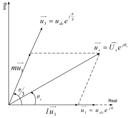
Figure 13. A voltage space vector in sector I
In Figure 13, over a switching period Ts, $\overrightarrow{u_{1}}$ and $\overrightarrow{u_{3}}$ are applied for time intervals of lTs and mTs respectively. $\overrightarrow{u_{0}}$ and $\overrightarrow{u_{7}}$ are the zero vectors applied for n0Ts and n7Ts respectively. Where n=n0+n7, and l+m+n =1.
$\overrightarrow{u_{s}^{a}}=\frac{1}{T_{s}}\left(l T_{s} \overrightarrow{u_{1}}+m T_{s} \overrightarrow{u_{3}}+n T_{s} .0\right)$ (64)
$\overrightarrow{u_{s}^{a}}=\overrightarrow{lu_{1}}+m \overrightarrow{u_{3}}$ (65)
Expressing Eq. (65) in polar form,
$\widehat{U}_{s} e^{j \theta_{s}}=l U_{d c} e^{j 0}+m U_{d c} e^{ \frac{j\pi}{3}}$ (66)
Solve Eq. (66) for time intervals by equating real and imaginary parts.
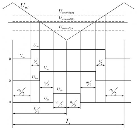
Figure 14. Sector-I pole voltages over time period (Ts)
In Figure 14, it was observed that pole-a have the prolonged time interval for ‘up’ position, following pole-b and then pole-c. Likewise, the switching can be done for any other sectors. Generation of the stator output voltage vector $\overrightarrow{u_{s}^{a}}$ with phase voltages $u_{a}, u_{b}$ and $u_{c}$, for specified $U_{d c}$ include, the comparison of control voltages with reference triangular signal $\widehat{U}_{t r i}$. For ASM, the stator winding is star connected with isolated neutral. So, $u_{a}(t)+u_{b}(t)+u_{c}(t)=0$.
$\left.\begin{array}{rl}\frac{\mathrm{U}_{\text {control }(\mathrm{a})}}{\widehat{\mathrm{U}}_{\text {tri }}}=\frac{\mathrm{u}_{\mathrm{a}}-\mathrm{u}_{\mathrm{k}}}{\left(\mathrm{U}_{\mathrm{dc}} / 2\right)} ; \frac{\mathrm{U}_{\mathrm{control}(\mathrm{b})}}{\widehat{\mathrm{U}}_{\text {tri }}}=\frac{\mathrm{u}_{\mathrm{b}}-\mathrm{u}_{\mathrm{k}}}{\left(\mathrm{U}_{\mathrm{dc} / 2}\right)} ; \frac{\mathrm{U}_{\mathrm{control}(\mathrm{c})}}{\widehat{\mathrm{U}}_{\text {tri }}}=\frac{\mathrm{u}_{\mathrm{c}}-\mathrm{u}_{\mathrm{k}}}{\left(\mathrm{U}_{\mathrm{dc}} / 2\right)} \\ \text { where } \mathrm{u}_{\mathrm{k}}=\frac{\max \left(\mathrm{u}_{\mathrm{a}}, \mathrm{u}_{\mathrm{b}}, \mathrm{u}_{\mathrm{c}}\right)+\min \left(\mathrm{u}_{\mathrm{a}}, \mathrm{u}_{\mathrm{b}}, \mathrm{u}_{\mathrm{c}}\right)}{2}\end{array}\right\}$ (67)
To set up largest magnitude in output voltage of stator voltage space vector $\overrightarrow{u_{s}^{a}}$, join the extreme points of the basic vectors to form a hexagon. Then inscribe a largest circle in hexagon. The inscribed circle radius is the maximum value of $\overrightarrow{u_{s}^{a}}$. The maximum value that $\overrightarrow{u_{s}^{a}}$ can accomplished from Figure 15.
Figure 15. Limit for maximum value output voltage
$\left|\overrightarrow{u_{s(\max )}^{a}}\right|_{p h}=\frac{2}{3} U_{d c} \cos \left(\frac{\pi}{3}\right)=\frac{1}{\sqrt{3}} U_{d c}$ (68)
$\left|\overrightarrow{u_{s(\max )}^{a}}\right|_{L-L(r m s)}=\sqrt{3} \frac{\left|\overrightarrow{u_{s(\max )}^{a}}\right|_{p h}}{\sqrt{2}}=\frac{U_{d c}}{\sqrt{2}}=0.707 U_{d c}$ (69)
In sinusoidal PWM inverter [14].
$\left|\overrightarrow{u_{s(\max )}^{a}}\right|_{L-L(r m s)}=\frac{\sqrt{3} U_{d c}}{2 \sqrt{2}}=0.612 U_{d c}$ (70)
On comparing SVPWM and SPWM from Eq. (69) and Eq. (70) the accessible output voltage is approximately 15% higher for SVPWM scheme. The Simulink model of SVPWM inverter is shown in Figure 18.
To illustrate the design of low pass filter, Butterworth filter approximation was considered because it advantages maximum flat response in magnitude, good roll-off to high frequencies, minimum phase and perfect bandwidth limitation [15]. Here second-order low-pass passive filter was designed. SOLP’s can also be structured by cascading of two first-order low- pass filters, but the cut-off frequency doesn’t remain same as cut-off frequency of first-order filter. For nth order filter the cut-off frequency varies as $\omega_{n c o}=\omega_{c o} \sqrt{2^{1 / n}-1}$. In Butterworth approximation the cascading of any order filters doesn’t affect the cut-off frequency. The circuit of SOLP passive filter is shown in Figure 16. Substitute s=jω and observe the behaviour of the filter for zero and infinite frequencies.
Figure 16. RLC second-order low-pass filter
For $\omega$= 0, the inductor will be short-circuited, while capacitor is open-circuited. The output voltage is nearly equal to the input voltage, and the voltage gain is close to unity. For $\omega=\infty$, inductor will be open-circuited while capacitor is short-circuited and voltage gain is zero. The filter admits all the signals for lower frequencies beneath cut-off frequency and attenuates for higher frequencies upon cut-off frequency. Thus, it acts as low-pass filter. The transfer function of the above filter circuit is shown in Figure 16 is given in Eq. (71).
$\frac{U_{o u t}(s)}{U_{i n}(s)}=\frac{1 / L C}{\left(s^{2}+\frac{R}{L} s+\frac{1}{L C}\right)}$ (71)
The transfer function of SOLP filter is given in Eq. (72).
$\frac{U_{o u t}(s)}{U_{i n}(s)}=\frac{\omega_{c o}^{2}}{\left(s^{2}+\frac{\omega_{c} s}{Q}+\omega_{c o}^{2}\right)}$ (72)
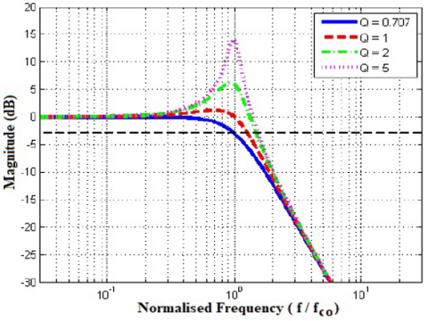
where, $\omega_{c o}$ is cut-off or resonant frequency in rad.s-1 and Q is quality factor. $\omega_{c o}=\frac{1}{2 \pi \sqrt{L C}}$, and $Q=\frac{1}{\omega_{c o} R C}=\frac{\omega_{c o} L}{R}$. In Figure 17, we observe the roll-off rate is 40 dB per decade and the amount of peaking was decided by the value of quality factor (Q). Maximally flat response was observed for Q = 0.707, which is Butterworth response. The Butterworth SOLP filter transfer function is given in Eq. (73). Similarly, one can design a SOLP with the quality factor (Q) equal to 2 and the transfer function of such SOLP filter with quality factor is given in Eq. (74) [15].
Figure 17. A Magnitude Vs frequency plot for SOLP filter
$\frac{U_{o u t}(s)}{U_{i n}(s)}=\frac{\omega_{c}^{2}}{s^{2}+1.414 \omega_{c} s+\omega_{c}^{2}}$ (73)
$\frac{U_{o u t}(s)}{U_{i n}(s)}=\frac{\omega_{c}^{2}}{s^{2}+0.5 \omega_{c} s+\omega_{c}^{2}}$ (74)
The switching frequency ($f_{s w}$) of SVPWM inverter is selected 10 kHz and it would be the cut-off frequency (fco). Substituting the value of $\omega_{c o}$, in Eq. (73), for $\omega_{c o}$=2πfco, and compared with Eq. (71). For a selected value capacitor (C) = 0.01µF, the values of resistance (R) and inductance (L) was determined. The corresponding values of R and L were found to be 2.25kΩ and 25.3mH respectively. Thus, the passive filter was developed by Butterworth approximation. Finally, the filtering is implemented by placing a transfer function per phase in the proposed Simulink model.
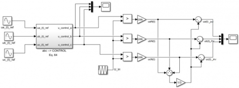
Simulation is performed in MATLAB for SVPWM inverter and IDSVC of ASM of electric vehicle as shown in Figure 18 and Figure 19 respectively.
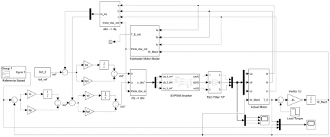
The output voltages of SVPWM inverter are not pure sinusoidal in nature and also at high speed operation of motor, the switching frequency of inverter does not remain constant. So, in order to reshape the output voltages and reject the wanted high frequency voltage signals a SOLP RLC filter is accommodated in conjunction with inverter. This is realized by placing a transfer function in the propounded Simulink model as shown in Figure 19. To simulate the model shown in Figure 19, it is required to run a program to calculate initial conditions and the algorithm 1 is implemented.
Figure 18. A SVPWM inverter Simulink model
Figure 19. A Simulink model of IDSVC of ASM
Algorithm 1. To determine initial conditions of drive
|
1. |
Consider the test motor specifications for Electric vehicle. Frequency (f) = 60 Hz, $u_{L-L(r m s)}$= 460 V, slip(s) = 0.0172, Rs = 1.77 Ω, Rr = 1.34 Ω , Xs = 144.25 Ω, Xr = 143.57 Ω, Xm = 139 Ω, J = 0.025 kg.m2, p = 4, $U_{d c}$= 700 V, $\mathrm{U}_{\text {tri }}$= 5 V and fsw = 104 Hz.[13] |
|
2. |
Consider the equivalent circuit of ASM referred to primary, calculate $\overrightarrow{u_{a}}, \overrightarrow{i_{a}}$, and $\overrightarrow{i_{r}}=\overrightarrow{-i_{r a}^{\prime}}$, using phasor analysis. |
|
3. |
Calculate $\overrightarrow{i_{s}^{a}}$ and $\overrightarrow{i_{r}^{a}}$ by considering a-axis as reference at time t=0 using dq analysis. |
|
4. |
Calculate machine inductances $L_{s}, L_{r}, L_{m}$ and $\tau_{r}$. find matrix [M]. |
|
5. |
For d-axis lined up to a-axis of stator at t = 0 ($\theta_{d s a}=0$), calculate $i_{s d}(0), i_{s q}(0), i_{r d}(0)$ and $i_{r q}(0)$ from Eq. (6) and Eq. (7), and then evaluate for $T_{E}(0)$ and actual rotor speed $\omega_{\operatorname{Mech}}(0)$ from Eq. (31) and Eq. (33). |
|
6. |
Calculate the flux linkages $\psi_{s d}(0), \psi_{s q}(0), \psi_{r d}(0)$ and $\psi_{r q}(0)$ from Eq. (34). |
|
7. |
In steady state, for $\omega_{d s a}=\omega_{s y n}$, all variables of d-q windings are dc in nature, then $\frac{d}{d t} \omega_{s d}=\frac{d}{d t} \omega_{s q}=0$, where $\omega_{s y n}=2 \pi f$. Calculate $\mathrm{u}_{\mathrm{sd}}(0)$ and usq(0) from Eq. (16) and Eq. (17). |
|
8. |
For d-axis aligned to rotor flux, $\psi_{r q}=0$. Calculate new values of $\psi_{r d}(0), \psi_{s d}(0), \psi_{s q}(0), i_{s d}(0), i_{s q}(0), u_{s d}(0)$ and $u_{s q}(0)$. |
|
9. |
Calculate the constants Kp and Ki of speed controller from Figure 10 [14]. Consider cross over frequency = 25 rad.s-1 and phase margin = 75 rad s-1. |
|
10. |
Calculate the constants Kpi and Kii of current controller from Figure 9 [13]. |
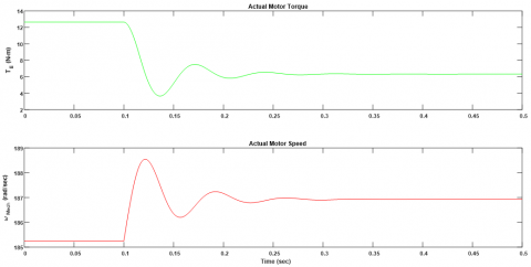
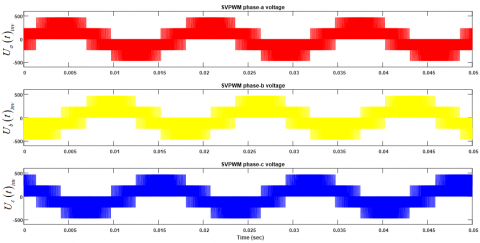
The ASM Simulink model shown in Figure 7 is simulated over a time period of 0.5 s and load torque is reduced to 50% of initial value at 0.1s. The electromechanical torque (TE) and mechanical speed ($\omega_{\mathrm{Mech}}$) plots are figured in Figure 20. It was observed that when the load torque is reduced, the speed is increased by a proper value. The Simulink model of SVPWM inverter shown in Figure 18 is simulated for a time period of 0.05 s. The 3-Փ voltage waveforms generated by SVPWM inverter is shown in Figure 21.
Figure 20. Torque and Speed plot when torque is reduced to half of its value at 0.1 sec of actual ASM
Figure 21. 3-Փ Phase voltages generated by SVPWM inverter
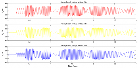
Figure 22. Unfiltered stator voltages
Figure 23. Filtered stator voltages
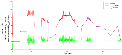
Figure 24. Torque and speed plots for IDSVC of ASM without SOLP RLC filter
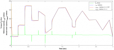
Figure 25. Torque and speed plots for IDSVC of ASM with both SOLP RLC filters wih Q = 0.707 and Q = 2
The block diagram shown in Figure 8 is modelled in Matlab / simulink as shown in Figure 19. A reference speed drive curve is considered over a time period of 3s and system is simulated. The stator voltage waveforms of SVPWM inverter connected without and with SOLP filter is shown in Figure 22 and Figure 23 respectively. In Figure 22, non-uniformity in waveforms is observed at higher amplitudes of stator voltages generated by SVPWM inverter in each of the three phases when operated without SOLP filter. Figure 24 and Figure 25 shows electromechanical torque and output mechanical speed plots when SVPWM inverter is connected without and with filter respectively. Actually, the SVPWM inverter injects required phase voltages into the stator windings. At high–speed (≥126 rad.s-1) operation of vehicle, the switching frequency ($f_{s w}$) of SVPWM inverter is inconsistent, which injects distorted voltages into stator windings of ASM. Spikes are observed in torque and speed plots during this high-speed range as shown in Figure 24. The adversity was mastered by placing a SOLP RLC filter with Butterworth approximation in conjunction with SVPWM inverter as shown in Figure 25.
The speed profile of the vehicle model with Butterworth approximation with quality factor equal to 0.707 is compared with another SOLP filter with quality factor equal to 2 as depicted in Figure 25. It was noticed that the speed profile with Butterworth approximation tracks the reference speed with in short period of time compared to other filter. This is because; in Butterworth approximation the magnitude of the speed has flat response without peaking. As the quality factor increases the peaking increases which require more time to settle and does not track the speed response perfectly.
In this paper, indirect space vector control of ASM for EV is modelled and simulated in Matlab / Simulink environment. The SVPWM power processing unit along with SOLP filter with Butterworth approximation was designed and modelled for high-speed functioning of the vehicle. The drive is tested for wide speed range with and without SOLC filter. Excellent torque and speed tolerant capabilities were found over the entire speed range, when connected with Butterworth approximated SOLP filter compared to SOLP filter with quality factor 2. Fluctuations occur in torque and speed profiles are obliterated. Uniformity in stator voltages generated by the SVPWM inverter is achieved. The vehicle speed follows the speed reference rapidly with improved transient performance and minimum speed regulation. Moreover, the viability of adopting the propounded scheme to high speed EV was met.
|
u, U |
voltage, V |
|
i |
current, A |
|
t |
time, s |
|
N |
dimensionless winding number |
|
T |
torque, N.m |
|
p |
dimensionless pole number, p ≥ 2 |
|
J |
combined inertia of load and motor, Kg.m2 |
|
a,b,c |
three phases of 3-Phase windings |
|
f |
frequency, Hz |
|
q |
switch logic position, 1or 0 |
|
K |
constant |
|
Q |
dimensionless quality factor |
|
Z |
dimensionless state transformation matrix |
|
MMF |
magneto motive force |
|
DC |
direct current |
|
PI |
proportional integral |
|
PM |
phase margin |
|
PPU |
power processing unit |
|
Greek symbols |
|
|
Փ |
phase |
|
α |
orthogonal α winding axis |
|
β |
orthogonal β winding axis |
|
σ |
dimensionless, leakage factor |
|
ϴ |
phase angle, (electrical) rad |
|
ω |
angular speed, ($\omega_{\mathrm{dsa}}, \omega_{\mathrm{dra}}, \omega_{\mathrm{m}}$ and $\omega_{\mathrm{syn}}$) in electrical rad.s-1 |
|
τ |
time constant, s |
|
ψ |
flux linkages, Wb |
|
Subscripts |
|
|
d-q |
direct and quadrature winding axis |
|
s |
Stator winding |
|
r |
Rotor winding |
|
L |
load |
|
E |
Electromagnetic |
|
m |
magnetizing |
|
m |
mechanical (for $\theta_{\mathrm{m}}$ or $\omega_{\mathrm{m}}$) |
|
Mech |
mechanical |
|
l |
leakage |
|
n |
neutral |
|
tri |
triangular |
|
ph |
phase |
|
nco |
nth order cut-off |
|
co |
cut-off |
|
in |
input |
|
out |
output |
|
sw |
switching |
|
syn |
synchronous |
|
Superscripts |
|
|
a |
reference phase –a |
|
T |
transpose of matrix |
|
→ |
Space vector |
|
˄ |
phasor |
|
ref |
reference |
|
est |
estimated |
(1) The MMF produced by stator 3-phase winding is defined as the ratio of number of stator winding turns per phase to pole number and multiplied by stator current. The space vector MMF produced by stator winding is with reference a-axis given by $\overrightarrow{M M F_{s}^{a}}(t)=\frac{N_{s}}{P} \overrightarrow{l_{s}^{a}}(t)$, where $\overrightarrow{l_{s}^{a}}(t)$ is space vector stator current, $N_{s}$ is number of turns per phase, p is pole number.
from Eq. $(5) \overrightarrow{i_{s}^{d}}(t)=\sqrt{\frac{3}{2}}\left(i_{s d}(t)+j i_{s q}(t)\right.$
Multiplying both sides by $\frac{N_{s}}{p}$
$\frac{N_{s}}{p} \overrightarrow{i_{s}^{d}}(t)=\frac{N_{s}}{p} \sqrt{\frac{3}{2}}\left(i_{s d}(t)+j i_{s q}(t)\right)$
The space vector stator current produced by three phase abc windings is independent of reference axis. On substituting $\overrightarrow{i_{s}^{d}}(t)=\overrightarrow{i_{s}^{a}}(t)$ in the above equation.
$\Rightarrow \frac{N_{s}}{P} \overrightarrow{i_{s}^{a}}(t)=\frac{\sqrt{\frac{3}{2}}\left(N_{s}\right)}{P}\left(i_{s d}(t)+j i_{s q}(t)\right) \Rightarrow \overrightarrow{{M M F}_{s}^{a}}(t)=\overrightarrow{{M M F}_{s}^{d}}(t)$
We have chosen the number of turns per phase of d-axis and q-axis winding to be $\sqrt{\frac{3}{2}}\left(\mathrm{~N}_{\mathrm{s}}\right)$. By definition of MMF it was proved that MMF produced by stator three phase abc windings is same as that of MMF produced by orthogonal stator d-q windings.
(2) The matrix M is invertible because, firstly it is a square matrix with the order 4X4 and secondly it is a non-singular matrix. The determinant of the matrix is non zero. For checking the non-singularity, calculate the determinant of the matrix, which is given by
$L_{s}^{2} L_{r}^{2}+L_{m}^{4}-L_{s} L_{r} L_{m}^{2}-L_{s} L_{r}^{2} L_{m}$
In the present model we have considered $X_{s}=144.25 \Omega, X_{r}=143.57 \Omega$ and $X_{m}=139 \Omega$ [13]. From the formula $X=2 \pi f L$, calculate the values of inductances and substitute in the above formula. We can find that the determinant of the matrix is non zero and hence it can be said that the matrix is invertible.
[1] Shafiei, S., Salim, R.A. (2014). Non-renewable and renewable energy consumption and CO2 emissions in OECD countries: A comparative analysis. Energy Policy, 66: 547-556. https://doi.org/10.1016/j.enpol.2013.10.064
[2] Rajashekara, K. (1994). History of electric vehicles in general motors. IEEE Transactions on Industry Applications, 30(4): 897-904. https://doi.org/10.1109/28.297905
[3] Attias, D. (2016). The Automobile Revolution: Towards a New Electro-Mobility Paradigm. Springer.
[4] Tvrdon, M., Chlebis, P., Hromjak, M. (2013). Design of power converters for renewable energy sources and electric vehicles charging. Advances in Electrical and Electronic Engineering, 11(3): 204-209. https://doi.org/10.15598/aeee.v11i3.795
[5] Sarlioglu, B., Morris, C.T., Han, D., Li, S. (2015). Benchmarking of electric and hybrid vehicle electric machines, power electronics, and batteries. In 2015 Intl Aegean Conference on Electrical Machines & Power Electronics (ACEMP), pp. 519-526. https://doi.org/10.1109/OPTIM.2015.7426993
[6] Windisch, T., Hofmann, W. (2015). Loss minimizing and saturation dependent control of induction machines in vehicle applications. In IECON 2015-41st Annual Conference of the IEEE Industrial Electronics Society, pp. 001530-001535. https://doi.org/10.1109/IECON.2015.7392318
[7] Koga, K., Ueda, R., Sonoda, T. (1992). Constitution of V/f control for reducing the steady-state speed error to zero in induction motor drive system. IEEE Transactions on Industry Applications, 28(2): 463-471. https://doi.org/10.1109/28.126757
[8] Patil, U.V., Suryawanshi, H.M., Renge, M.M. (2014). Closed-loop hybrid direct torque control for medium voltage induction motor drive for performance improvement. IET Power Electronics, 7(1): 31-40. https://doi.org/10.1049/iet-pel.2012.0509
[9] Krishnan, R., Bharadwaj, A.S. (1991). A review of parameter sensitivity and adaptation in indirect vector controlled induction motor drive systems. IEEE Transactions on Power Electronics, 6(4): 695-703. https://doi.org/10.1109/63.97770
[10] Perdukova, D., Fedor, P. (2014). A model-based fuzzy control of an induction motor. Advances in Electrical and Electronic Engineering, 12(5): 427-434. https://doi.org/10.15598/aeee.v12i5.1229
[11] Ong, C.M. (1998). Dynamic simulation of electric machinery: Using MATLAB/SIMULINK, 5. Upper Saddle River, NJ: Prentice hall PTR.
[12] Chau, K.T. (2015). Electric Vehicle Machines and Drives: Design, Analysis and Application. John Wiley & Sons.
[13] Mohan, N. (2014). Advanced Electric Drives: Analysis, Control, and Modeling Using MATLAB/Simulink. John Wiley & Sons.
[14] Mohan, N. (2012). Electric Machines and Drives: A First Course (No. 621.31042 M697e). Wiley.
[15] Schaumann, R., Mac Elwyn Van Valkenburg, X., Xiao, H. (2001). Design of Analog filters, 1. New York: Oxford University Press.