Basma Ismail | Mahmoud Abo El Enin | Mariam Osama | Mariam Abdelhaleem | Michael Geris | Mohamed Kamel | Sally Kassem* | Irene S. Fahim
© 2021 IIETA. This article is published by IIETA and is licensed under the CC BY 4.0 license (http://creativecommons.org/licenses/by/4.0/).
OPEN ACCESS
Route optimization is tactically important for companies that must fulfill the demands of different customers with fleet of vehicles, considering multiple factors like: the cost of the resources (vehicles) involved and the operating costs of the entire process. As a case study, a third-party logistics service provider, ABC Company, is introduced to implement optimization on. Furthermore, ABC Company’s problem is defined as route optimization and load consolidation problems that will be solved as heterogeneous vehicle routing problem with soft time windows (HVRPSTW). In this paper’s case, Vehicles travel from a central depot with a restricted capacity, serving clients just once within a defined time interval and providing a needed demand before returning to the central depot. ABC Company’s problem is mathematically formulated and solved using branch and bound method. The formulation is solved on LINGO. The final output is the route, time, cost, and load of each vehicle.
heterogeneous vehicle routing problem, soft time windows, mixed integer programing, case study
The classical VRP is one of the most important problems studied within the field of transportation optimization. This is due to the significant cost encountered in the transportation process. Since the problem has been introduced for the first time [1], it has been subject to numerous research. VRP, creates ideal delivery routes in which each vehicle only takes one route that starts from a centralized depot. The VRP's aim is to discover a set of least-cost vehicle routes in which each client is visited precisely once by one vehicle, each vehicle begins and ends its route at the depot, and the vehicle capacity is not overloaded [2-4]. The problem has been viewed and modeled from different perspectives and using several techniques, for example mathematical models [5], agent based VRP [6], and unified modeling language modeling [7]. The traditional VRP has been expanded in a variety of ways by including new real-life elements or traits, leading to a massive number of VRP variations. Extensions include changing the capacities of vehicles, resulting in the Heterogeneous Fleet VRP (HFVRP), also recognized as the Mixed Fleet VRP [8]. In VRP with time windows (VRPTW), which is another common extension, customers are often only available over a specific period. This adds up constraints on delivery/picking time, as the vehicle must visit a customer within a defined time frame [9, 10]. Failing to visit customers within their determined time window results in customer dissatisfaction. Another variant of the problem is the Vehicle routing Problem with Pickup and Delivery (VRPPD), in which each vehicle will pick up items/passengers at location A and drop them off at location B. On demand transport is a typical case – delivering services that satisfy consumer demands directly (e.g., taxi, shuttle service, buses, etc.). Routing results in paired pick-up and delivery points aligned with origin and destination. Goods must be picked up from a specific place and delivered to their destination. Because the pick-up and drop-off must be done by the same truck, the pick-up and drop-off locations must be included in the identical route. A similar issue is the VRP with backhauls (VRPB), in which a car does both deliveries and pick-ups along the same route. Some clients demand deliveries (known as line hauls), while others want pick-ups (referred to as backhauls). The combination of line hauls and backhauls has shown to be quite beneficial to the industry [1].
VRP with time windows could be categorized as VRP with hard time windows and VRP with soft time windows. In case of hard time windows, vehicles routing is done with the objective of minimizing total trip cost, and customers must be visited within their time windows without any flexibility in violating these time windows constraints. On the other hand, in VRP with soft time windows, the same objective holds, but visiting customers outside the predefined time windows of a customer is permitted at an additional cost known as penalty. The penalty is usually added to the trip cost and is proportional to the amount of time windows violation [11].
Heterogeneous vehicle routing problem with soft time windows (HVRPSTW) is an updated model from the VRP with soft time windows, where a set of customers are served using a fleet of heterogeneous vehicles. Vehicles with different capacities are located at a central depot, and are required to deliver customers’ demands. Customers’ coordinates and their associated demands are known before the start of the trip. Customers’ demands are assigned to vehicles, and hence vehicles depart to deliver demand to customers in a sequence that minimized the entire transportation costs of all customers’ deliveries, and at the same time, customers are to be visited as much as possible within their preset time windows. Time window violation is allowed at a cost. The time window violation cost is added to the transportation cost to be minimized [12]. After visiting the assigned customers, each vehicle ends the trip at the depot. VRP and its variants are NP hard in nature. Hence, only small size problems could be solved using exact methods to obtain optimal solutions [2]. Practical size problems require other solution methods like heuristics and metaheuristics. When adding time windows constraints and variability of truck types, VRP will be solved accurately with respect to the company’s given specific constraints and problem size. This will aid in saving costs by decreasing number of trips made and reducing time windows’ violation.
1.1 Related work
The authors [13] discuss a heterogeneous fleet VRP modeled by including the entire trip load constraint into the goal function. The problem is solved using a sequential inclusion heuristic with a punishment function that allows capacity breaches but limits them to a changeable specified upper bound. Periodic Heterogeneous Vehicle Routing Problem (PHVRP) is introduced in the reference [14]. The paper aim is to schedule deliveries based on viable combinations of delivery days, as well as to set fleet and driver scheduling and vehicle routing regulations. The authors [15] illustrate a Construction of a variety of velocity profiles along road segments, which are subsequently translated into traveling-time tables. A case study of rice distribution across communities by the bureau of logistics is presented to find the best option in terms of vehicle routes and service start times.
Column generation is used to solve the LP relaxation of the VRPTW’s set partitioning formulation [16]. An iterative route construction procedure is introduced in the reference [17] to solve the VRP with soft time windows as well as VRP with hard time windows. The proposed solution algorithm has quality and computing time that are comparable to existing solutions on benchmark problems. VRP with time windows in cross docking stations is presented in, and the problem in solved using Tabu Search and Variable Neighborhood Search methods [2, 18]. VRP with hard time windows and stochastic service times is formulated as a set partitioning problem and is solved using precise branch-cut-and-price algorithms [19]. The algorithm depends on creating efficient labelling algorithms by selecting appropriate label components and establishing lower and higher bounds on partial route decreased cost to be utilized in the column production phase. A case study considering distribution of liquefied petroleum gas in Turkey is discussed by Onut et al. [20], where the paper presents a model of heterogeneous vehicles used to deliver goods such that the total demand cannot exceed the vehicle capacity and the model was solved using GAMS for optimum solutions. Most studies in the field of VRP and its extensions focus on modelling the problem variants and/or developing heuristics or metaheuristics methods to solve large size problems. However, few research work addressed the variant of soft time windows. Moreover, and to the best of our knowledge, no research has addressed the topic of heterogeneous vehicle routing problem with soft time windows within the assumptions and constraints given in this work.
In this paper, a heterogeneous vehicle routing problem with soft time windows (HVRPSTW) is modeled to represent an existing case study in Egypt, as case studies are good for describing, comparing, evaluating and understanding different aspects of a research problem, and allows in-depth, multi-faceted explorations of complex issues in real-life settings. To the best of our knowledge, the developed model with the details representing the case study is a novel mixed integer linear programming mathematical model. To offer a solution to the company of the case study, the developed model is solved to optimality using LINGO software.
The rest of this paper is organized as follows: Section 2 provides a detailed description of the problem statement representing the case study, Section 3 illustrates the methodology adopted to solve the problem in hand, in Section 4 results obtained for the data of the case study are presented and, finally, Section 5 concludes the paper.
ABC Company is a delivery company that offers transportation solutions for fast moving consumer goods (FMCG) companies. It combines logistics technologies with high quality service to offer customized delivery solutions in the Middle East and North Africa (MENA) region. To provide full control and visibility over the driver, ABC Company connect FMCG companies with a wide network of trucks with different types and capacities to serve as a fleet.
The services that ABC Company offers include paperless transactions, multiple drop offs, data analytics, time & motion study, drivers, tailored operation process, capacity utilization, cash collection, and backhauling logistics. Cashless transactions service is coming soon.
ABC Company’s problem is misallocation of vehicles’ resources. They allocate any vehicle type or size to the customer even if the truck capacity is larger than the required demand resulting in a more expensive trip and, hence an unsatisfied customer. Moreover, Company ABC does not have the concept of consolidation.
The problem this paper solves is summarized as follows: ABC company is utilizing a fleet of heterogeneous vehicles. The fleet of vehicles is located at several locations that are close to each other and hence, may be approximated as being located at a central depot. ABC company receives several FMCG orders from customers. These orders are to be first collected from several warehouse locations, and then, delivered to several demand points. ABC company collects all orders, select the appropriate vehicle(s) to be dispatched from the central depot to visit the appropriate warehouses to collect the demanded orders, and then visit the customers to deliver the demand orders, and finally return to the central depot. Warehouses are closely located, and are all within the proximity of the depots, and hence, warehouses are also approximated to be coinciding with the location of the central depot. Accordingly, depots and warehouses are approximated to be the central depot (one single node) from where vehicles loaded with customers’ demands are dispatched to serve customers. Dispatched vehicles carry demand that does not exceed the capacity of any vehicle. Each customer is visited by one vehicle during a pre-determined time window set by the customer. If the vehicle arrives earlier or later than the time window boundaries, a penalty is encountered that increases the overall trip cost. For example, if a vehicle arrives earlier than the earliest time defined by the customer, the demand drops off start immediately but a penalty is added. Similarly, if the vehicle arrives later than the latest arrival time determined by the customer, a penalty is added.
As a group of customers is served by a diverse fleet of vehicles. Vehicles of various capacities depart from a central depot to meet the needs of customers and return to the central depot at the end of the trip (Heterogeneous Vehicle Routing Problem). Vehicles are allowed to service customers before and after the earliest and latest time window bounds in this problem (soft time windows) but with penalties. Hence, the problem in hand described in the problem definition could be categorized as Heterogeneous Vehicle Routing Problem with Soft Time Windows (HVRPSTW). Similar analysis is seen in [12], with different problem details and assumptions.
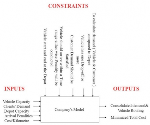
Figure 1. Block diagram to illustrate ABC Company model
Figure 1 illustrates how to build a model that represents the activities performed in ABC company, starting with the system inputs which are divided into Vehicle capacity illustrating the maximum capacity the vehicle can load, Clients’ Demand explains the needed amount of load to be delivered to customer , Depot Capacity is the maximum amount of load the depot can store, Arrival Penalties illustrate the fine price which will be included if the driver arrives early/late to the customer and finally, Cost/Kilometer illustrates the cost applied for each kilometer , constraints are divided into 5 main which are: To calculate demand compared to Depot which shows that the demand of client should be equal or less than the maximum load of depot, Vehicle has one Drop-off or more, this constraint shows that a vehicle can have more than a client to drop off some load at, Customer Demand should be satisfied, here the constraint explains that the customer demand should be equal or less than the supply we have, Vehicle should arrive within a Time range otherwise a penalty will be conducted, this constraint illustrates that arriving out of the time range will apply penalty on the driver and finally, Vehicle start and end at the depot, here the constraint is allowing the vehicle to start the trip from depot and finish it at the same depot. and finally the model outputs need to reduce travel costs and improve coordination between different deliveries.
In this paper, the problem is mathematically formulated. The developed mathematical model is solved using LINGO software to obtain an optimum solution.
3.1 Mathematical formulation
A mixed integer linear programming model for the HVRPTW problem of the case study is formulated and given below.
The parameters used in the mathematical formulation are:
N: Number of nodes.
K: Maximum number of vehicles to employ.
Qk: Capacity of vehicle type k.
$C_{i j}$: Transportation cost between node i and node j, where node 0 represents the site of the depot; i, j = 0, 1, 2… N and $C_{i j}$=0.
$P E_{-} C_{i}$: Early penalty cost for customer i, if vehicle arrives before the earliest allowed start time at node i, the service will start with considering this penalty cost; i= 1, 2... N and $P E_{-} C_{0}$= 0 where 0 is a central depot.
$P L_{-} C_{i}$: Late penalty cost for customer i, if vehicle arrives after the latest allowed start time at node i, the service will start with considering this penalty cost; i= 1, 2... N and $P L_{-} C_{0}=$= 0 where 0 is a central depot.
$T_{i j}$: Travel time between node i and node j, i, j = 0, 1, 2… N and $T_{i i}$ = 0.
$E_{j}$: Earliest allowed start time of service for the customer at node, j = 1, 2…N.
$L_{j}$: Latest allowed start time of service for the customer at node, j = 1, 2…N.
$S r_{j}$: Service time for the customer at node, j = 1, 2…N.
$d_{j}$: Amount of products to deliver to the customer at node j, j = 1, 2….N.
M: large positive number.
Decision Variables:
$x_{i j k}\left\{\begin{array}{c}1 \text { if vehicle } \mathrm{k} \text { travels from node } \mathrm{i} \text { to } \\ \mathrm{j} \mathrm{i}, \mathrm{j}=0 \ldots \ldots, N \\ 0 \quad \text { otherwise }\end{array}\right.$
$P E_{-} T_{j k}\left\{\begin{array}{c}1, \text { if service start time for customer } \\ \mathrm{j}, S t_{j}<E_{j}, j=1, \ldots, N \\ 0 \quad \text { otherwise }\end{array}\right.$
$P L_{-} T_{j k}\left\{\begin{array}{c}1, \text { if service start time for customer } \\ \mathrm{j}, S t_{j}>L_{j}, j=1, \ldots, N \\ 0 \quad \text { otherwise }\end{array}\right.$
$S t_{j}$: start of service time at customer j, j = 1,…,N.
$l d_{k}$: load of vehicle k at the start of the trip.
Objective Function:
The model's objective function is to minimize the total transportation costs, including penalties for arriving earlier or later than the time windows. The objective function is:
Min $=\sum_{i=0}^{N} \sum_{j=0}^{N} \sum_{k=1}^{K} C_{i j k} X_{i j k}+$
$\sum_{j=1}^{N} \sum_{\mathrm{k}=1}^{K} P E_{-} C_{j} * P E_{-} T_{j k}+\sum_{\mathrm{j}=1}^{N} \sum_{\mathrm{k}=1}^{K} P L_{-} C_{j} *$
$P L_{-} T_{j k}$ (1)
Constraints:
The objective function is subject to the following constraints:
$\sum_{i=0}^{N} \sum_{k=1}^{K} X_{i j k}=1 \quad j=1, \ldots, N$ (2)
$l d_{k}=\sum_{i=0}^{N} \sum_{i=1}^{N} d_{j} X_{i j k} \forall k \in K$ (3)
$l d_{k} \leq Q_{k} \quad \forall \mathrm{k} \in \mathrm{K}$ (4)
$\sum_{i=0}^{N} \mathrm{x}_{\mathrm{ibk}}-\sum_{j=0}^{N} \mathrm{x}_{\mathrm{bjk}}=0 \quad b=1, \ldots N, \forall \mathrm{k} \in \mathrm{K}$ (5)
$M \times P E_{-} T_{j k}+S t_{j} \geq E_{j}$ (6)
$-M \times\left(1-P E_{T_{j k}}\right)+S t_{j}<E_{j}$ (7)
$-M \times P L_{-} T_{j k}+S t_{j} \leq L_{j}$ (8)
$M \times\left(1-P L_{T_{j k}}\right)+S t_{j}>L_{j}$
$j=2 \ldots \ldots N, k=1,2 \ldots \ldots . K$ (9)
$S t_{i}+T_{i j}+S r_{i}-M \times\left[1-x_{i j k}\right] \leq S t_{j}$
$i=0 \ldots N, j=2 \ldots N, k=1 \ldots K$ (10)
$X_{i j k}=\{0,1\} i, j=1, \ldots \ldots N, k=1,2 \ldots \ldots . K$ (11)
$P E_{-} T_{j k}=\{0,1\} j=2, \ldots \ldots N, k=1,2 \ldots \ldots . K$ (12)
$P L_{-} T_{j k}=\{0,1\} j=2, \ldots \ldots N, k=1,2 \ldots \ldots . . K$ (13)
Constraint (2) assures that vehicle k visits node j from node i only once. In constraint (3), the load of a vehicle is calculated according to the demand for all nodes j assigned to the vehicle. Constraint (4) assures that the total load assigned to a vehicle does not exceed the vehicle’s capacity. Constraint (5) states that when a vehicle visits a node will ultimately leave it (flow conservation constraint). Constraints (6) and (7) determine whether the vehicle visits a node earlier than the earliest allowable time of the time window, and accordingly, determines the amount of violation and the penalty for early arrival, if exists. Constraints (8) and (9) determine whether the vehicle visits a node later than the latest allowable time of the time window, and accordingly, determines the amount of violation and the penalty for late arrival, if exists. Constraint (10) calculates the start of service time, which equals to the arrival time, at customers’ nodes. Constraints (11) to (13) are binary constraints.
3.2 ABC company’s cost structure
Table 1. Oil changes
|
Vehicle Types |
Oil changes 3000Km (105 LE/Liter) |
Cost of 1 0il filter/LE |
Total (LE) |
|
T series (Consumes 7 Liter) |
735 |
100 |
835 |
|
N series (Consumes 8 Liter) |
840 |
200 |
1040 |
A cost structure was prepared to set a pricing criterion for the contractors. The cost structure depends on the influencing factors that affect the costs of a trip, directly and indirectly and on the short and long term such as the running costs (oil /3000 Km, diesel consumption/ liter 100 Km, loaded vehicle diesel consumption, tires and the deteriorated engine consumption (it is calculated based on each 800 Km) for the two types of trucks used in ABC Company (N series (6 tires) and T series (4 tires) as shown in the Tables 1-5. After calculating the overall cost which includes diesel price / liter/100 Km, it will be used in the mathematical formulation to minimize the trip cost.
Table 2. Diesel consumption
|
Vehicle Types |
Diesel consumption (liters/100km) |
Diesel Price consumed (liters/100km)/L.E. |
|
T series |
12.8 |
64 |
|
N series |
13.6 |
93 |
Table 3. Loaded diesel consumption
|
Vehicle Types |
Diesel consumption (liters/100km) |
Diesel price consumed (liters/100km)/L.E. |
|
T series (Loaded 1 Ton) |
94.5 |
85.6 |
|
N series (Loaded 4.25 ton) |
130.4 |
195 |
Table 4. Tires
|
Vehicle Types |
Cost of Tires/L.E. |
|
T series (4 Tires) |
4890 |
|
N series (6 Tires) |
12765 |
Table 5. Deteriorated engine consumption
|
Vehicle Types |
Diesel consumption increased for each 8000 Km |
Diesel price increased/L.E./Km |
|
T Series |
753 |
0.09425 |
|
N Series |
1181 |
0.1476 |
3.3 Software implementation
To test the effectiveness of the model, it is using a linear programming software. This study applies the model on LINGO software, the following data is gathered and assembled on ABC Company’s routing problem. Some of the data is collected by calculating the time and the destination using Google Maps. It represents a limited form of the data to test the efficiency of the model. ABC Company requires a centered depot among the nodes to be reachable by every destination. They deal with the following locations:
The six locations mentioned are represented by nodes from 1 to 6, respectively. The first node (depot) has a capacity of 100 units and the system operates with two vehicles with capacities of 50 and 80 units. The cost/km according to the cost structure is 3.16 L.E. The rest of the data such as: demand, early and late hours, service time, travel time, and early/late penalty cost are represented in Tables 6, 7 in the form of nodes and matrices that satisfy these nodes. Data in Tables 8, 9 are extracted from a web mapping platform between each node.
HVRPSTW model requires these data in order to operate vehicles with different capacities to fully optimize vehicles, depot capacity that vehicles must meet, time window range to check the arrival time to each node, and finally penalty cost which is applied to both late and early arrivals.
Table 6. Demand units, early & late minutes, and service time at each node
|
Nodes |
Demand Units |
Early Minutes |
Late Minutes |
Service Time Minutes |
|
1 |
0 |
0 |
200 |
0 |
|
2 |
20 |
60 |
80 |
10 |
|
3 |
30 |
0 |
120 |
10 |
|
4 |
30 |
0 |
90 |
10 |
|
5 |
10 |
90 |
130 |
10 |
|
6 |
10 |
90 |
100 |
10 |
Table 7. Randomly generated numbers for penalties
|
Early Penalty Cost |
Late Penalty Cost |
|
1 |
1 |
|
20 |
20 |
|
65 |
65 |
|
100 |
100 |
|
90 |
90 |
|
80 |
80 |
|
170 |
170 |
|
50 |
50 |
|
200 |
200 |
|
120 |
120 |
Table 8. Distance between defined nodes in Km
|
Nodes |
1 |
2 |
3 |
4 |
5 |
6 |
|
1 |
0 |
26 |
20 |
28 |
28 |
23 |
|
2 |
26 |
0 |
14 |
56 |
17 |
48 |
|
3 |
20 |
14 |
0 |
52 |
24 |
42 |
|
4 |
28 |
56 |
52 |
0 |
49 |
12 |
|
5 |
29 |
17 |
24 |
49 |
0 |
40 |
|
6 |
23 |
48 |
42 |
12 |
49 |
0 |
Table 9. Travel Time in minutes between nodes
|
Nodes |
1 |
2 |
3 |
4 |
5 |
6 |
|
1 |
0 |
38 |
33 |
42 |
41 |
33 |
|
2 |
38 |
0 |
27 |
58 |
31 |
55 |
|
3 |
33 |
27 |
0 |
53 |
38 |
56 |
|
4 |
42 |
58 |
53 |
0 |
55 |
26 |
|
5 |
41 |
31 |
38 |
55 |
0 |
62 |
|
6 |
33 |
55 |
56 |
26 |
62 |
0 |
4.1 Cost structure
When such cost structure is formulated, ABC Company will be able to stabilize the prices they pay for a trip which came out to be 3.16 L.E./km = 0.20$/Km on a systematic base to hinder the fluctuations in the prices they pay for the contractor on a single trip. The results of the cost structure will be used as an input in the objective function.
4.2 Solved model
The model is categorized as (non-deterministic polynomial-time hardness) NP hard type of models, which was solved using LINGO software and after implementing the model on LINGO the following results were concluded: vehicle 1 was loaded with 60 units while vehicle 2 was loaded with 40 units with a total of 100 which is satisfying needed demand and the capacity of the depot (node 1) as shown in Table 10 below.
Table 10. Capacity and load of each vehicle and capacity of depot
|
|
V1 |
V2 |
Depot |
|
Capacity |
80 Unit |
50 Unit |
100 Unit |
|
Load |
60 Unit |
40 Unit |
100 Unit |
The model was solved with a total of 4404 solver iterations, 169 solver steps, 116 variables and 130 constraints; to have a final objective function value minimized to 451.88 L.E.
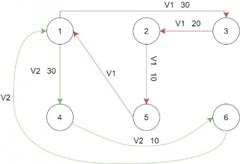
Table 11 and Figure 2 describe the two vehicles routing and drop offs loads were Vehicle 1 will start from Point 1 (Ezz Al Arab) with loaded capacity of (60 Unit) to Drop-off (30 Unit) at Point 3 (Dandy) and then drop-off (20 Unit) at Point 2 (Mall of Arabia) and finally, last drop-off of (10 Unit) at Point 5 (Mall of Egypt) and returning again to Point 1. On the other hand, Vehicle 2 will start from Point 1 (Ezz Al Arab) with loaded capacity of (40 Unit) to drop-off (30 Unit) at Point 4 (CFC) and then drop-off (10 Unit) at Point 6 (City Center Almaza) and finally, returning again to Point 1 (Ezz Al Arab).
Figure 2. Vehicles’ routes for the case study after solving the model
Table 11. From/to chart for each service point
|
From/to |
Ezz Al Arab Agouza |
Mall of Arabia |
Dandy |
CFC |
Mall of Egypt |
City center Almaza |
|
Ezz Al Arab Agouza |
0 |
0 |
30/V1 |
30/V2 |
0 |
0 |
|
Mall of Arabia |
0 |
0 |
0 |
0 |
10/V1 |
0 |
|
Dandy |
30/v1 |
0 |
0 |
0 |
0 |
0 |
|
CFC |
0 |
0 |
0 |
0 |
0 |
10/V2 |
|
Mall of Egypt |
0/V1 |
0 |
0 |
0 |
0 |
0 |
|
City center Almaza |
0/V2 |
0 |
0 |
0 |
0 |
0 |
Vehicle routing problem (VRP) has been a significant topic in logistics and transportation management study in recent years, and it is frequently utilized in transportation systems, logistics distribution systems, and express delivery systems. The goal of solving VRP is to discover delivery routes that can meet both supplier and clients in the same route without generating additional costs. The concept of the research concentrates mainly on a case study of a single-depot heterogeneous VRP with soft time windows since it is a critical issue to investigate to achieve its goal, therefore a linear programming model has been formulated, which contains a specific objective function subject to various constraints. The problem is NP- hard in nature. Lingo software was used as a method to validate the model and acquire the most optimum solution. Future work will be based on conducting a more in-depth examination of the best VRP solution at various multiple depot transportation demand model & further implementation on LINGO software.
[1] Dantzig, G.B., Ramser, J.H. (1959). The truck dispatching problem. Management Science, 6(1): 80-91. https://doi.org/10.1287/mnsc.6.1.80
[2] Kassem, S., Korayem, L., Khorshid, M., Tharwat, A. (2019). A hybrid bat algorithm to solve the capacitated vehicle routing problem. In 2019 Novel Intelligent and Leading Emerging Sciences Conference (NILES), 1: 222-225. https://doi.org/10.1109/NILES.2019.8909300
[3] Shalaby, M., Mohammed, A., Kassem, S. (2021). Supervised fuzzy C-means techniques to solve the capacitated vehicle routing problem. International Arab Journal of Information Technology, 18(3A): 452-463. https://doi.org/10.34028/iajit/18/3A/9
[4] Shalaby, M.A.W., Mohammed, A.R., Kassem, S. (2020). Modified fuzzy c-means clustering approach to solve the capacitated vehicle routing problem. In 2020 21st International Arab Conference on Information Technology (ACIT), pp. 1-7. https://doi.org/10.1109/ACIT50332.2020.9300082
[5] Toth, P., Vigo, D. (2002). An overview of vehicle routing problems. The Vehicle Routing Problem, 1-26. https://doi.org/10.1137/1.9780898718515.ch1
[6] Vokrínek, J., Komenda, A., Pˇechoucek, M. (2010). Agents towards vehicle routing problems. In AAMAS. 773-780.
[7] Abdullatif, N., Kassem, S. (2020). Modelling of agent-based vehicle routing problem using unified modelling language. Journal Européen des Systèmes Automatisés, 53(6): 781-789. https://doi.org/10.18280/jesa.530604
[8] Baldacci, R., Battarra, M., Vigo, D. (2008). Routing a heterogeneous fleet of vehicles. In The Vehicle Routing Problem: Latest Advances and New Challenges, 43: 3-27. https://doi.org/10.1007/978-0-387-77778-8_1
[9] Kallehauge B., Larsen J., Madsen O.B., Solomon M.M. (2005). Vehicle routing problem with time windows. In: Desaulniers G., Desrosiers J., Solomon M.M. (eds) Column Generation. Springer, Boston, MA. https://doi.org/10.1007/0-387-25486-2_3
[10] Braekers, K., Ramaekers, K., Van Nieuwenhuyse, I. (2016). The vehicle routing problem: State of the art classification and review. Computers & Industrial Engineering, 99: 300-313. https://doi.org/10.1016/j.cie.2015.12.007
[11] Mustafa, M., Abdel Salam, H., Kassem, S. (2018). Vehicle routing problems with simultaneous pickup and delivery soft time window. International Journal of Academic Management Science Research, 2(9): 1-7.
[12] Kang, H.Y., Lee, A.H. (2018). An enhanced approach for the multiple vehicle routing problem with heterogeneous vehicles and a soft time window. Symmetry, 10(11): 650. https://doi.org/10.3390/sym10110650
[13] Rabbani, M., Taghi-Molla, A., Farrokhi-Asl, H., Mobini, M. (2019). Sustainable vehicle-routing problem with time windows by heterogeneous fleet of vehicles and separated compartments: Application in waste collection problem. International Journal of Transportation Engineering, 7(2): 195-216. https://doi.org/10.22119/IJTE.2019.94586.1361
[14] Panggabean, E.M., Mawengkang, H., Azis, Z., Sari, R.F. (2018). Periodic heterogeneous vehicle routing problem with driver scheduling. In IOP Conference Series: Materials Science and Engineering, 300(1): 012017. https://doi.org/10.1088/1757-899X/300/1/012017
[15] Hanum, F., Hartono, A.P., Bakhtiar, T. (2018). On the multiple depots vehicle routing problem with heterogeneous fleet capacity and velocity. In IOP Conference Series: Materials Science and Engineering, 332(1): 012052. https://doi.org/10.1088/1757-899X/332/1/012052
[16] Desrochers, M., Desrosiers, J., Solomon, M. (1992). A new optimization algorithm for the vehicle routing problem with time windows. Operations Research, 40(2): 342-354. https://doi.org/10.1287/opre.40.2.342
[17] Figliozzi, M.A. (2008). An iterative route construction and improvement algorithm for the vehicle routing problem with soft and hard time windows. https://www.researchgate.net/publication/228669883_An_iterative_route_construction_and_improvement_algorithm_for_the_vehicle_routing_problem_with_soft_and_hard_time_windows.
[18] Sadri Esfahani, A., Fakhrzad, M.B. (2014). Modeling the time windows vehicle routing problem in cross-docking strategy using two meta-heuristic algorithms. International Journal of Engineering, 27(7): 1113-1126. https://doi.org/10.5829/idosi.ije.2014.27.07a.13
[19] Errico, F., Desaulniers, G., Gendreau, M., Rei, W., Rousseau, L.M. (2016). A priori optimization with recourse for the vehicle routing problem with hard time windows and stochastic service times. European Journal of Operational Research, 249(1): 55-66. https://doi.org/10.1016/j.ejor.2015.07.027
[20] Onut, S., Kamber, M.R., Altay, G. (2014). A heterogeneous fleet vehicle routing model for solving the LPG distribution problem: A case study. In Journal of Physics: Conference Series, 490(1): 012043. https://doi.org/10.1088/1742-6596/490/1/012043