Mulukala Sri Lalith | Patthi Sridhar* | Ranjith Kumar Gatla | Alladi Sathish Kumar
© 2021 IIETA. This article is published by IIETA and is licensed under the CC BY 4.0 license (http://creativecommons.org/licenses/by/4.0/).
OPEN ACCESS
This paper is devoted to describe how surge magnitudes are calculated and how do we use this data in order to determine the ageing of insulation on the transmission line poles so that we can replace the insulation in pre fault time, based on its condition. The main object of this report is to design algorithm of implementation of SCADA in the transmission line system to identify insulation ageing factor. In order to identify the magnitude of voltage due to direct lightning source, we have some formulae which provides the approximate value. For the magnitude value due to indirect lightning strokes, we use two methods namely RBF-FDTD method which uses artificial neural network function in order to study the detailed concept of coupling between field to transmission lines and the other method is the modelling of simulation system in which the coupling system approximations are taken. This paper also describes about the calculation of outage rate and its Geometrical analysis.
surge magnitude, radial basis function, finite difference time domain
There are two types of overvoltage in a power system: lightning impulse and switching impulse [1]. Switching impulses are triggered by changes in the system's operation. When lightning strikes power system equipment, it causes lightning impulses. Negative and positive lightning are the two forms of lightning that can be triggered based on the type of electrical discharge, with the latter being about 10 times greater than the former [2]. Cloud to Ground (CG), Ground to Cloud (GC), and Cloud to Cloud (CC) are the three general classifications based on charge flow. Direct lightning strikes on power systems are triggered by CG and CC, while induced lightning effects in power systems can be caused by any kind of lightning.
Since the effects of lightning strokes can be seen in the power system equipment, earthing of all power system equipment, including transmission line poles, is needed. The transmission line poles' footing resistance and the earth mat of the substations should be held at low values to achieve better protection from lightning. In order to achieve maximum protection, the earth resistance is usually kept below 10Ω [3]. The earth resistance is maintained about 1-2Ω in some high-altitude areas. Transmission cables, poles, overhead lines near the substation, and the substation itself are the places where lightning strikes are most likely to occur.
Electrical transmission system is adopted to transfer electricity from generating station to the load centres, electricity travels around hundred to thousands of kilometers through these transmission lines. Here the voltage is raised 400kv or other high value with the help of power transformers to reduce the losses. Lightning strikes transmission lines in both direct and indirect (induced) ways [4]. Poles are used to link transmission cables from the source to the destination. There's a risk that lightning could strike the tops of poles, inducing lightning surges in the phase conductors. The poles must be grounded in order to prevent the transients in the system [5]. The conduction between the pole and the overhead line cables is stopped with the help of high insulations which prevents the cables from direct contact to the pole.
For the selection of an appropriate insulation level and the design of an effective protection scheme in medium voltage lines, the assessment of lightning flashover rate is unavoidable [6, 7]. Because lightning stroke variables are stochastic in nature, peak lightning-induced overvoltage’s (LIVs) also vary wildly. The flashover voltage of line insulation exposed to a specific voltage stress, on the other hand, is stochastic in nature. Given the randomness of the magnitude and shape of LIVs, as well as the widely dispersed probabilities of insulation flashover voltages, employing a risk-based insulation coordination method is more realistic [8, 9].
The worst-case scenario for a lightning strike is overhead lines near to substations. Both the substation and the transmission are damaged when lightning hits overhead lines near the substation [10]. If the lightning protection systems fail to stop it, it has the potential to cause significant damage to the system equipment. The magnitude of the surge current is divided into two parts and drives into the system. Lightning protection systems have been installed in the substations. To divert the direction of surge to the ground, all of the equipment in the substation is grounded. In order to divert surges to ground, various forms of earthing and grounding practices are used. The lightning rod is taken as a lightning protection scheme.
In order to identify the Induced effect of lightning on the transmission line system we have to identify the effect of electromagnetic fields in the overhead cables CC lightning often serves as an indirect lightning stroke in certain high-altitude regions, influencing system parameters.
2.1 Calculation of EMF across the line
In order to calculate the electromagnetic fields (EMF) the current channel is considered as a function of altitude and time i(z',t). The Induced lightning current is a function of current obtained on the basis of current channel i(o,t) As it is the only form of current which can be measured directly [11].
$i(0, t)=I_{0}\left(e^{(-\alpha t)}-e^{(-\beta t)}\right)$ (1)
I0 - magnitude of surge currents produced due to Induced effect of lightning.
α, β are constants,
$i\left(z^{\prime}, t\right)=i\left(0, t-z^{\prime} / v\right) e^{\left(-z^{\prime} / \lambda\right)}$ (2)
The model that describes the relationship between indirect lightning and phase line fields is used to calculate the emf equation of the lightning return stroke. We must consider the Maxwell theory in both scalar and vector potentials in order to obtain the horizontal and vertical components of the emf equation.
$\varphi=\frac{1}{4 \pi \varepsilon_{0}} \int_{(V)} \frac{t-R / C}{R} d V$ (3)
$\bar{A}=\frac{\mu}{4 \pi} \int_{(V)} \frac{\bar{J}(t-R / C)}{R} d V$ (4)
when there is a known potential in the system, the electric field is calculated by using the following equation:
$\bar{E}=-\operatorname{grad} \varphi-\frac{\partial \bar{A}}{\partial t}$ (5)
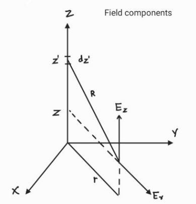
Figure 1. Field component coordinate system
X axis - transmission line.
Y axis - to determine distance between point of strike to cable.
Z axis - to analyse vertical dipole.
By considering the ground as a reference conductor, we derive the equations of electromagnetic fields of horizontal and vertical dipoles with help of coordinate system as shown in Figure 1. The Figure 1 describes the information about field component coordinate ordination system in which we consider a 3D axis in order to identify the point of strike which lies at a particular distance from transmission line. The overall fields consist of three different components of fields they are:
Electrostatics: It consists of the field effects of static charged particles and it is directly proportional to integral of current.
Electrostatics $\propto \int$ current.
Induction: This effect changes with the change in currents of the system.
Induction $\propto$ current.
Radiation: This effect changes with the rate of change of current with respect to time.
Radiation $\propto \frac{\partial(\text { current })}{\partial t}$.
The overall vertical dipole EMF (EZ) is written as:
Ez = Ez1 + Ez2+Ez3 (6)
where,
$E_{z 1}(r, z, t)=\frac{1}{4 \pi \varepsilon_{0}} \int_{-z^{\prime}}^{z^{\prime}}\left(\frac{2\left(z-z^{\prime}\right)^{2}-r^{2}}{R^{5}} e^{\left(-z^{\prime} / \lambda\right)} \cdot \int_{0}^{t} i\left(0, \tau-z^{\prime} / V-R / c\right) d \tau\right) d z^{\prime}$ (7)
$E_{z 2}(r, z, t)=\frac{1}{4 \pi \varepsilon_{0}} \int_{-z^{\prime}}^{z^{\prime}}\left(\frac{2\left(z-z^{\prime}\right)^{2}-r^{2}}{c R^{4}} e^{\left(-z^{\prime} / \lambda\right)} \cdot i\left(0, t-z^{\prime} / V-R / c\right)\right) d z^{\prime}$ (8)
$E_{z 3}(r, z, t)=\frac{1}{4 \pi \varepsilon_{0}} \int_{-z^{\prime}}^{z^{\prime}}\left(\frac{r^{2}}{c^{2} R^{3}} e^{\left(-z^{\prime} / \lambda\right)}\right.$.
$\left.\frac{\partial i\left(0, t-z^{\prime} / V-R / c\right)}{\partial t}\right) d z^{\prime}$ (9)
For Er, the EMF of horizontal dipole is written as:
$E_{r}=E_{r 1}+E_{r 2}+E_{r 3}$ (10)
where,
$E_{r 1}(r, z, t)=\frac{1}{4 \pi \varepsilon_{0}} \int_{-z^{\prime}}^{z^{\prime}}\left(\frac{3 r\left(z-z^{\prime}\right)}{R^{5}} e^{\left(-z^{\prime} / \lambda\right)} \cdot \int_{0}^{i} i\left(0, \tau-z^{\prime} / V-R / c\right) d \tau\right) d z^{\prime}$ (11)
$E_{r 2}(r, z, t)=\frac{1}{4 \pi \varepsilon_{0}} \int_{-z^{\prime}}^{z^{\prime}}\left(\frac{3 r\left(z-z^{\prime}\right)}{c R^{4}} e^{\left(-z^{\prime} / \lambda\right)} \cdot i\left(0, t-z^{\prime} / V-R / c\right) d z^{\prime}\right.$ (12)
$E_{r 3}(r, z, t)=\frac{1}{4 \pi \varepsilon_{0}} \int_{-z^{\prime}}^{z^{\prime}}\left(\frac{r\left(z-z^{\prime}\right)}{c^{2} R^{3}} e^{\left(-z^{\prime} / \lambda\right)}\right.$.
$\frac{\partial i\left(0, t-z^{\prime} / V-R / c\right)}{\partial t} d z^{\prime}$ (13)
where, i(0,t) is the current at channel base.
C = $3 \times 10^{8}$ m/s (speed of light).
$R=\sqrt{\left(r^{2}+\left(z-z^{\prime}\right)^{2}\right)}$ (14)
The value of z is altitude (taking ground as reference) where the field is calculated (z=h).
In order to obtain the value of time t we integration limit is set w.r.to z.
$z^{\prime} / v+\sqrt{\left(r^{2}+\left(z-z^{\prime}\right)^{2}\right) / c}=t$ (15)
2.2 Identification of overvoltage magnitude using EMF
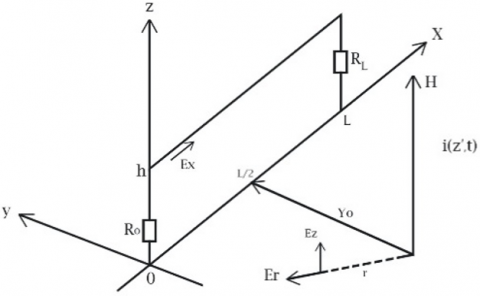
In order to design a coupling system which calculates the induced over voltages due to indirect lightning we have to project the components of Er (11) to (13) on the x-Er axis. The purpose of getting x-Er axis is to shift the point of strike to the cable point as we are supposed to calculate emf at cable not on the point of strike. This is done by the following equation which provides relation between Ex and Er [12].
$E_{x}(r, z, t)=E_{r}(r, z, t)(L / 2-x) / r$ (16)
Figure 2. Geometry of surge calculations
The field parameters are calculated for ground with high conductive property with the steps.
Step 1: Vertical parameters of the field.
Step 2: Frequency domain vertical components using DFT.
Step 3: Frequency domain horizontal components using transfer function.
$W(j \omega)=\frac{E_{r}(j \omega)}{E_{z}(j \omega)}=\left(\varepsilon_{r}+\frac{\sigma_{g r}}{j \omega \varepsilon_{0}}\right)^{-\frac{1}{2}}$ (17)
The above equation includes permittivity and conductivity of the ground which is displayed in Figure 2.
Step 4: Time domain horizontal components using IDFT.
The induced voltage due to indirect lightning stroke is calculated with the help of modifications in the normal form of travelling wave equation, this considers only a certain portion of the transmission line, this makes a modification in the system basic equations.
$\frac{\partial u^{s}(x, t)}{\partial x}+L^{\prime} \frac{\partial i(x, t)}{\partial t}=E_{x}^{i}(x, h, t)$ (18)
$\frac{\partial i(x, t)}{\partial x}+C^{\prime} \frac{\partial u^{s}(x, t)}{\partial t}=0$ (19)
The equation in time domain are as follows,
$u^{s}(t, x)=v\left(t-\tau_{x}\right)+w\left(t-\tau_{l-x}\right)$ (20)
$Z_{c} i(t, x)=v\left(t-\tau_{x}\right)-w\left(t-\tau_{l-x}\right)$
$+Z_{c} \frac{1}{L} \int_{0}^{t} E_{x}^{i}(t) d t$ (21)
The surge calculation is done in MATLAB which intakes the following parameters as an input to the code.
$r=\sqrt{Y_{0}^{2}+\left(\frac{L}{2}-(p-1) \cdot \frac{L}{N}\right)^{2}}$ (22)
It takes the numerical value of sections present in the transmission line system.
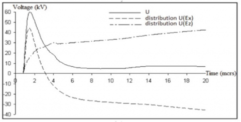
Figure 3. The induced voltages at x = 0m
Figure 4. The induced voltage at x = 250m
2.3 Direct formula for magnitude of induced voltage
Whenever an indirect lightning strikes nearby the transmission line system, the surge Ui will be injected into the system due to the coupling of magnetic field H. The induced voltage waveform for different values of x is shown in Figure 3 and Figure 4. Here, x is the distance between point of strike to the line, at x = 0 meters it is almost a direct lightning strike so the distribution Ex is positive, and at x = 250 meters, it is an indirect lightning strike, so as time increases it has to compensate. There is a direct formula which provides us with the approximate value of the induced voltage surge, it was given by Rusck [13].
$U_{\max , i}=Z_{0} i_{b} \frac{h}{x}$ (23)
where,
Z0 - mutual impedance (between line and strike point);
h - height of line with respect to the ground;
x - displacement between line and strike point;
ib- surge current induced in the transmission line.
Modified version of this formula is given as,
$U_{\max }=\frac{z_{0} I_{0} h}{d}\left(1+\frac{1}{\sqrt{2}} \frac{v}{c} \frac{1}{\sqrt{1-\frac{1}{2}\left(\frac{v}{c}\right)^{2}}}\right)$ (24)
where,
d - displacement between line and strike point;
v - return stroke velocity;
c = $3 \times 10^{8}$ m/s (speed of light).
2.4 RBF-FDTD method
This approach is used to solve the numerical equations in the coupling of the field produced by the lightning to the transmission line model. This method's output is the precise value of the lightning-induced overvoltage. The Radial Basis Function (RBF) and the Finite Difference Time Domain (FDTD) method are integrated in this method [2]. It provides comprehensive data on electromagnetic coupling in different phases of the power system (distribution and transmission phase). Advantages of FDTD is you can use to analyse electromagnetic fields for a time varying field, RBF is used to make nonlinear data point into linear.
2.4.1 Introduction to FDTD assumptions
The Maxwell’s equations are used in the finite difference time domain system to formulate the upcoming electric and magnetic field values. Based on the initial parameters, these formulae are used to predict the upcoming electric and magnetic field values [14]. The initial x-t plane must be used to construct a finite difference grid, which divides the overall plane into equipotential grids of steps, respectively $\Delta x$ and $\Delta t$. By considering The first and second order spatial derivatives of the function f(x,t) at a grid point, as well as the second order estimates of centred difference, are provided below.
$\frac{\partial}{\partial x} f(x, t)=\frac{f_{k+1}^{n}-f_{k-1}^{n}}{2 \Delta x}$ (25)
The second derivative of the above equation is given as:
$\frac{\partial^{2}}{\partial x^{2}} f(x, t)=\frac{f_{k+1}^{n}-2 f_{k}^{n}+f_{k-1}^{n}}{\Delta x^{2}}$ (26)
The first order time related derivative is given as:
$\frac{\partial}{\partial t} f(x, t)=\frac{f_{k}^{n+1}-f_{k}^{n-1}}{2 \Delta t}$ (27)
2.4.2 RBF FDTD Formulation
The mth order derivative of a function with respect to x, at a point xi, is approximated by the summation given below.
$\left.\frac{d^{m} f}{d x^{m}}\right|_{x_{i}}=\sum_{j=1}^{n} w_{i, j}^{m} f\left(x_{j}\right)$ (28)
The radial basis function is given as:
$f(x)=\sum_{j=1}^{n} \lambda_{j} \phi\left(\left\|\underline{x}-\underline{x}_{j}\right\|\right)+\beta$ (29)
The above equation includes RBF, $\|.\|$ is considered to be the norm.
We use multiquadric RBF to get the derived approximations in a one-dimensional (1D) domain as shown in Figure 5.
Figure 5. Support points for i in 1D domain
The first and second order spatial derivatives of finite difference and the first order derivative of temporal finite difference are given as:
$\frac{\partial}{\partial x} f(x, t)=k_{x}^{1}\left(f_{k+1}^{n}-f_{k-1}^{n}\right)$ (30)
$\frac{\partial^{2}}{\partial x^{2}} f(x, t)=k_{x}^{2}\left(f_{k+1}^{n}+f_{k-1}^{n}-2 f_{k}^{n}\right)$ (31)
$\frac{\partial}{\partial t} f(x, t)=k_{t}^{1}\left(f_{k}^{n+1}-f_{k}^{n-1}\right)$ (32)
The approximations of the radial basis function corresponding to the geometrical parameters of c are:
$k_{x}^{1}=\frac{\Delta x}{\left(\sqrt{4 \Delta x^{2}+c^{2}}-c\right) \sqrt{\Delta x^{2}+c^{2}}}$ (33)
$k_{x}^{2}=\frac{\frac{c^{2}}{\left(\sqrt{\Delta x^{2}+c^{2}}\right)^{3}}-\frac{1}{c}}{3 c-\sqrt{\Delta x^{2}+c^{2}}+\sqrt{4 \Delta x^{2}+c^{2}}}$ (34)
$k_{t}^{1}=\frac{\Delta t}{\left(\sqrt{4 \Delta t^{2}+c^{2}}-c\right) \sqrt{\Delta t^{2}+c^{2}}}$ (35)
when c tends to ∞ the approximations generated are same in both the methods [15]. In order to select a parameter for the spatial domain, we consider different values which provide a better result than the FDTD method [16]. The induced voltage calculation geometry is depicted in Figure 6.
We consider the coupling equation FTL (field to transmission lines (lossless)).
$\frac{\partial V^{s}(x, t)}{\partial x}+L \frac{\partial}{\partial t} I(x, t)=E_{x}^{i}(x, t)$ (36)
$\frac{\partial I(x, t)}{\partial x}+C \frac{\partial}{\partial t} V^{s}(x, t)=0$ (37)
where, $V^{s}(x, t)$ and $I(x, t)$ are the surges induced into the line due to FTL coupling.
Figure 6. Induced voltage calculation geometry
L and C are the inductance and capacitance (per unit length).
By differentiating the Eqns. (36) and (37) with respect to x, we get the second order equations as shown below:
$\frac{\partial^{2} V^{s}(x, t)}{\partial x^{2}}-L C \frac{\partial^{2} V^{s}(x, t)}{\partial t^{2}}=\frac{\partial E_{x}^{i}(x, t)}{\partial x}$ (38)
$\frac{\partial^{2} I(x, t)}{\partial x^{2}}-L C \frac{\partial^{2} I(x, t)}{\partial t^{2}}=-C \frac{\partial E_{x}^{i}(x, t)}{\partial t}$ (39)
By considering the Taylor series for the surges generated in the system up to second order is given as:
$\begin{aligned} V^{s}(x, t)=V^{s}(x,&\left.t_{0}\right)+\Delta t \frac{\partial V^{s}(x, t)}{\partial x} \\+& \frac{\Delta t^{2}}{2 !} \frac{\partial^{2} V^{s}(x, t)}{\partial t^{2}}+O\left(\Delta t^{3}\right) \end{aligned}$ (40)
$\begin{aligned} I(x, t)=I\left(x, t_{0}\right) &+\Delta t \frac{\partial I(x, t)}{\partial x}+\frac{\Delta t^{2}}{2 !} \frac{\partial^{2} I(x, t)}{\partial t^{2}} \\ &+O\left(\Delta t^{3}\right) \end{aligned}$ (41)
By substituting the values of first and second order derivatives of surges (time-based domain).
$V^{s}(x, t)=V^{s}\left(x, t_{0}\right)-\Delta t C^{-1} \frac{\partial I(x, t)}{\partial x}+\frac{\Delta t^{2}(L C)^{-1}}{2}\left(\frac{\partial^{2} V^{s}(x, t)}{\partial x^{2}}-\frac{\partial E_{x}^{i}(x, t)}{\partial x}\right)+O\left(\Delta t^{3}\right)$ (42)
$I(x, t)=I\left(x, t_{0}\right)-\Delta t L^{-1}\left(\frac{\partial V^{s}(x, t)}{\partial x}-E_{x}^{i}(x, t)\right)+\frac{\Delta t^{2}(L C)^{-1}}{2}\left(\frac{\partial^{2} I(x, t)}{\partial x^{2}}+C \frac{\partial E_{x}^{i}(x, t)}{\partial t}\right)+O\left(\Delta t^{3}\right)$ (43)
By representing the above equations in the spatial and time related derivatives using RBF-FDTD approximation are given as:
$V_{k}^{n+1}=V_{k}^{n}-\Delta t C^{-1} k_{x}^{1}\left(I_{k+1}^{n}-I_{k-1}^{n}\right)+\frac{\Delta t^{2}(L C)^{-1}}{2}\left[k_{x}^{2}\left(V_{k+1}^{n}+V_{k-1}^{n}-2 V_{k}^{n}\right)-k_{x}^{1}\left(E_{k+1}^{n}-E_{k-1}^{n}\right)\right]$ (44)
$I_{k}^{n+1}=I_{k}^{n}+\Delta t L^{-1}\left(E_{k}^{n}-k_{x}^{1}\left(V_{k+1}^{n}-V_{k-1}^{n}\right)\right)+\frac{\Delta t^{2}(C L)^{-1}}{2}\left[k_{x}^{2}\left(I_{k+1}^{n}+I_{k-1}^{n}-2 I_{k}^{n}\right)+C k_{t}^{1}\left(E_{k}^{n+1}-E_{k}^{n-1}\right)\right]$ (45)
The approximations are given as:
$V_{k}^{n} \equiv \mathrm{V}^{s}((k-1) \Delta x, n \Delta t)$ (46)
$I_{k}^{n} \equiv \mathrm{I}((\mathrm{k}-1) \Delta x, n \Delta t)$ (47)
where, $\Delta x, \Delta t$ are spatial and time steps (equal grid steps).
k, n are kth and nth integral steps (k is spatial and n is temporal).
The conditions to the boundaries of the surge voltage with a load at two-line closing is given as follows:
$V_{1}^{n}=\int_{0}^{h} E_{z}^{i}(0,0, t) d z-Z_{0} I_{1}^{n}$ (48)
$V_{N x+1}^{n}=\int_{0}^{h} E_{z}^{i}(L, 0, t) d z-Z_{L} I_{N x+1}^{n}$ (49)
where, $E_{z}^{i}$ refers to the incident electrical field (with respect to vertical field lines).
Z refers to the impedance of the termination of boundary lines.
The terminating conditions are designed in order to avoid the reflected waves on the boundaries [12].
The overall surge voltage induced into the transmission line system due to the indirect lightning stroke is given as a sum of the voltage scattered and the incident vertical electric field with a finite integral ranging from 0 to h.
$V^{T}(x, t)=V^{s}(x, t)-\int_{0}^{h} E_{z}^{i}(x, h, t) d z$ (50)
The above equation can be expressed as the sum of scattered and incident voltage.
$V^{T}(x, t)=V^{s}(x, t)+V^{i}(x, t)$ (51)
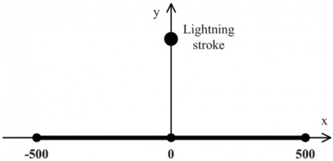
Figure 7. Distance between line and stroke
A perpendicular is drawn from the point of incidence of lightning to the transmission line considering the observation point at 500m, the 1D varies in the range [-500, 500] as shown in Figure 7. The results of magnitude of surge voltage due to lightning is shown in the Figure 8. 3D surface plot (voltage vs distance vs time).
Figure 8. Induced voltage plot
Direct lightning stroke is a case where the lightning directly come in contact with the power system equipment, in a transmission line system this case is considered if the lightning directly hits the cables or transmission line poles. If no proper protection system is equipped the it will cause a severe damage to the system [17]. In order to protect the system from these strokes we employee different protection schemes.
The surge current flows in both the directions, the overall magnitude of the current is divided into two equal parts. By knowing the value of surge impedance, we can find the overvoltage magnitude of the lightning stroke.
Let’s consider that the surge current Induced here is ib = 30kA.
The surge impedance Z = 200 ohms.
Then the surge voltage,
U = Z × ib (52)
U = 200 × 30 = 6000kV
For the above, the surge voltage Induced in transmission line due to direct lightning is 6000kV.
When a direct lightning strikes on the top of Pole or on earth Wire (shielding protector) under ideal conditions (zero Pole resistance) the complete surge current will be moved directly into the ground. But in practical conditions the Pole resistance can never be zero, so the surge is produced in the Pole, the surge produced is more than the withstand value of insulation which leads to a generation of flash between the Pole and the phase conductor.
Let’s consider that the surge current Induced here is ib = 30kA.
The pole resistance RE,P = 100 ohms.
Then the surge voltage,
U = RE,P × ib (53)
U = 100 × 30 = 3000kV
The value of surge obtained is higher than the withstand value of insulation which resulting in addition of surge into the phase wire due to back flash mechanism. In order to avoid this, we have to maintain the least possible resistance of the pole and we should maintain high withstand value insulation in the transmission line system. In order to absorb the surges raised in the system due to the lightning effect we employee voltage sensing equipment which helps in identifying the magnitude of surges in the system. The voltage sensing part has a stray capacitance C1 between the conductor and tank and a potential divider capacitance C2 in the pre amplification stages. We can also predict whether the surge formed due to direct or indirect lightning stroke with the help of polarities of the surges. The surge polarities are constant in all the phases for the Induced lightning effect but in the direct lightning effect the polarities differ in all the phases. These are arranged at the switching substations and the surges can be recorded by the continuous monitoring of the phase lines of the transmission line. The magnitude of voltage across the line is measured with the help of the impact dividers (voltage dividers capacitance) and stray capacitance and the value is enhanced in the further procedure in order.
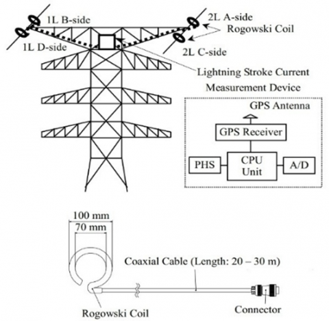
In order to perform the study on lightning strike effects on transmission line we employee certain instrumentation in the transmission line which helps to identify the Amplitude of the surges encountered in the system. This is known as an observatory system. In the UHV lines we employee the observatory system in order to study the surge that encountered in the earth Wire of the transmission line.
This system analyses the potential in the earth Wire with the help of Rogowski coil arranged at both the sides of the earth Wire shield as shown in Figure 9. The measurement device shown in Figure 9 are lightning surge invasions were captured through continuous line voltage observation using voltage sensors (mostly voltage sensor including stray capacitance/ voltage capacitance divider) installed on the detector terminal at the GIS space of switching stations/substations. The recorded data is transmitted with the help of GPS to the personal handset (PHS) and we do have analog to digital converter in order to obtain the value of the surge current due to lightning stroke on the ground Wire.
Figure 9. Observatory system for UHV TL
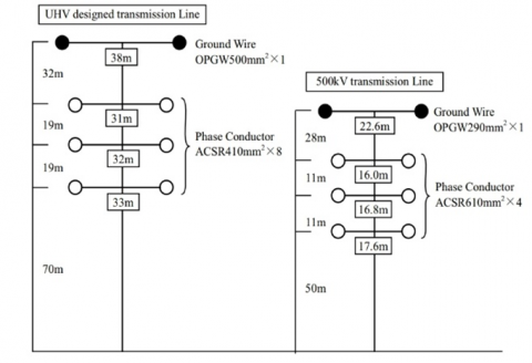
These arrangement plans shown in Figure 10 are designed to reduce the effect of lightning and to increase the probability of lightning to fall on the earth Wire shielding in order to reduce the chances of high surges generated in the phase wires of the UHV lines.
Figure 10. Conductor positioning in the UHV transmission lines
Outage rate gives the relation between the lightning shielding success and its failure. It mostly describes about the shielding success in the transmission line system. If the lightning shielding works efficiently, outages can be eradicated from the system. The lightning outage in a transmission line system causes back flashover voltages. The lightning outage at different conductors is shown in Figure 11.
Figure 11. Examples of lightning outage at different conductors
4.1 Outage rate calculation
The IEEE standards provide us with the formulae applied to find the lightning density on the ground. Generally, ground flash density is calculated based on LLC (lightning location system) and LFC (lightning flash counters) but these are inaccurate, So instead we calculated Ng as below (Only one location per flash us considered).
$N_{g}=0.04 T_{d}^{1.25}$ (54)
$N_{g}=0.054 T_{h}^{1.1}$ (55)
where, $N_{g}$ is the Lightning density on the ground (GLD).
$T_{d}$ is the count of thunderstorm days.
$T_{h}$ is the count of lightning hours.
For every 100 kilometres line being hit by lightning surges each year is described as:
$N=N_{g}\left(\frac{28 H_{T}^{0.6}+b}{10}\right)$ (56)
$N=N_{g}\left(\frac{4 h_{p}^{1.09}+b}{10}\right)$ (57)
$N=N_{g}\left(\frac{38 h_{p}^{0.45}+b}{10}\right)$ (58)
where, N is the count of lightning strikes.
$h_{p}$ - height of line with respect to ground.
$H_{T}$ - tower height with respect to ground.
b - ground wire spacing.
The function of return stroke current is given as:
$f_{i}(I)=\left(\frac{1}{\sqrt{2 \pi} \sigma_{l n} I}\right) e^{\frac{-(\ln I / \bar{I})^{2}}{2 \sigma_{l n}^{2}}}$ (59)
where, $\sigma_{l n}$ for current less than 20kA.
$\bar{I}$ is the reference current.
If the amplitude of the return stroke > the collective, requires $f_{i}(I)$.
The probability can also be given as:
$P\left(I_{f}>I\right)=\frac{1}{1+\left(\frac{I}{\bar{I}_{\text {first }}}\right)^{2.6}}$ (60)
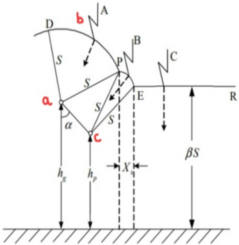
4.2 Geometrical analysis
In order to understand the concept of lightning strike in the transmission line environment, we consider the geometrical analysis which provides the protection angle value in order to increase the shielding efficiency. This analysis is known as Electrical shielding geometry. We use this model in order to analyse the failure in shielding which consists of ground wire on the top of the tower and reference ground component. Let us consider, α as a protection angle, the striking distance is given by S and its factor is given as β. The model of the considered case is shown in Figure 12.
Figure 12. Geometrical model (Xs ≠ 0)
where, DPER- path of lightning pilot.
a- line of lightning.
b - point of lightning strike.
c - describes the phase line.
Due to increase in the magnitude of surge current (due to lightning) the distance of striking will also increase. Due to this, the distance PE will gradually decrease and becomes 0 eventually.
Figure 13. Geometrical model (Xs = 0)
where, point P is known as critical point.
The Figure 13 describes the model where Xsis absent, at this point, the conductor is completely shielded due to maximum surge current shielding and maximum strike distance.
We do observe sag in the conductor which results in the new height of the phase line with respect to the ground. We need to identify the average height of the phase line which is provided by the given formula.
$H_{p}=h_{p}-\frac{2}{3} S_{a p}$ (61)
where, $S_{a p}$ denotes sag observed in the phase line.
If the strike distance is identified and the product of the strike distance factor and the strike distance is less than the height of phase line (considering sag).
$X_{s}=S\left[\cos \theta+\sin \left(\alpha_{s}-\omega\right)\right]$ (62)
$\theta=\sin ^{-1}\left(\frac{\beta S-H_{p}}{S}\right)$ (63)
$\omega=\cos ^{-1}\left(\frac{\sqrt{\left(x_{p}-x_{g}\right)^{2}+\left(H_{p}-H_{g}\right)^{2}}}{2 S}\right)$ (64)
$\alpha_{s}=\tan ^{-1}\left(\frac{x_{p}-x_{g}}{H_{g}-H_{p}}\right)$ (65)
These are obtained with the help of horizontal coordinates of phase and ground wires. Under this condition.
$X_{s}=S\left[1+\sin \left(\alpha_{s}-\omega\right)\right]$ (66)
whenever there is a minimum amount of surge current the exposure distance is maximum and the exposure distance is 0 corresponding to maximum surge current [18].
$N_{S F}=0.1 N_{g} \frac{X_{s}}{2}\left(P_{\min }-P_{\max }\right)$ (67)
where, Pmin is the probability of the surge current amplitude being above Imin.
Pmax is the probability of the surge current amplitude being above Imax.
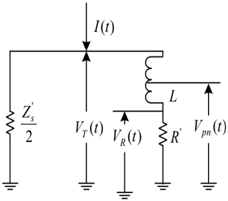
In HV transmission lines, whenever a direct lightning strikes on the top of the pole it produces a back flash if the insulation failure occurs.
Let us consider a voltage calculation model with respect to resistance and inductance.
Figure 14. Electrical circuitry of tower
In Figure 14, we have considered tower or the pole as a transmission line.
where,
$Z_{S}^{\prime}=\frac{2 Z_{S} Z_{T}}{Z_{S}+2 Z_{T}}$ (68)
$R^{\prime}=\frac{R Z_{T}}{Z_{T}-R}$ (69)
By considering the time of propagation and the attenuation coefficient we get the values.
$Z_{W}=\frac{2 Z_{T} Z_{S}^{2}}{\left(2 Z_{T}+Z_{S}\right)^{2}} \frac{Z_{T}-R}{Z_{T}+R}$ (70)
$\psi=\frac{2 Z_{T}-Z_{S}}{2 Z_{T}+Z_{S}} \frac{Z_{T}-R}{Z_{T}+R}$ (71)
where, $\psi$ is the coefficient of attenuation.
With these parameters, we can find out the total inductance of the tower.
$L=\left(\frac{Z_{S}^{\prime}+2 R^{\prime}}{Z_{S}^{\prime}}\right) \frac{2 Z_{w} \tau_{T}}{(1-\psi)^{2}}$ (72)
We use volt time characteristics of lightning current to calculate the value of voltage at which the critical breakdown takes place.
Whenever the lightning strike takes place, we have to calculate the voltage on the insulation at only two points. Let us consider the time divisions as 2-6 micro seconds. Let’s consider two cases in calculating the value of voltage at insulator.
Case 1 - Non reflective case
$V_{T 2}=\left[Z_{1}-\frac{\mathrm{Z}_{w}}{1-\psi}\left(1-\frac{\tau_{T}}{1-\psi}\right)\right] I$ (73)
The impedance is given as:
$Z_{i}=\frac{Z_{s} Z_{T}}{Z_{s}+2 Z_{T}}$ (74)
Case 2 - Reflective case
$V_{T 2}^{\prime}=\left[Z_{1}-\frac{-4 \mathrm{~K} V_{T 2}}{Z_{s}}\left(1-\frac{\tau_{T}}{Z_{s}}\right)\right]\left(1-\tau_{s}\right)$ (75)
This includes the coefficient of attenuation (considering Ks = 0.85 in this case).
If the current propagation time is greater than one microsecond then it come under a non-reflective case (at time = 2 micro seconds). When the propagation time is less than one microsecond.
$V_{T 2}=V_{T 2}+V_{T 2}{ }^{\prime}$ (76)
The grounding voltage at time is equals 2+τT is given as:
$V_{R 2}=\left[\frac{\alpha_{1} Z_{1}}{1-\psi}\left(1-\frac{\psi \tau_{T}}{1-\psi}\right)\right] I$ (77)
$\alpha_{1}=\frac{2 R}{z_{T^{+R}}}($ Grounding current related $)$ (78)
$V_{p n 2}=V_{R 2}+\frac{\tau_{T}-\tau_{p n}}{\tau_{T}}\left(V_{T 2}-V_{R 2}\right)$ (79)
$\tau_{p n}$ is the time of transmission from pole top to the n bars of magnitude of surge current.
The voltage of the nth number phase line is given as the difference between the voltage of insulator strings to the phase voltage.
$V_{s n 2}=V_{p n 2}-K_{n} V_{T 2}$ (80)
At a time, t = 6 micro seconds, the pole has lost its impact resistance as the peak of surge current has passed. So, the voltage is given as:
$V_{T 6}=\left(\frac{Z_{s} R}{Z_{s}+2 R}\right) I$ (81)
For a reflecting case, the voltage expression is given as:
$V^{\prime}{ }_{T 6}=-4 K_{s} Z_{s}\left(\frac{R}{Z_{s}+2 R}\right)^{2}\left(1-\frac{2 R}{Z_{s}+2 R}\right) I$ (82)
The insulator voltage is given as:
$V_{s n 6}=\left[V_{T 6}+V_{T 6}^{\prime}\right]\left(1-K_{n}\right)$ (83)
The voltage of insulators at two microseconds and 6 microseconds is given as:
$V_{I 2}=820 l$ (84)
$V_{16}=585 l$ (85)
where, l is the length of insulation.
The flash over currents is given as:
$I_{c n 2}=\frac{V_{I 2}}{V_{s n 2}}$ (86)
$I_{c n 6}=\frac{V_{I 6}}{V_{s n 6}}$ (87)
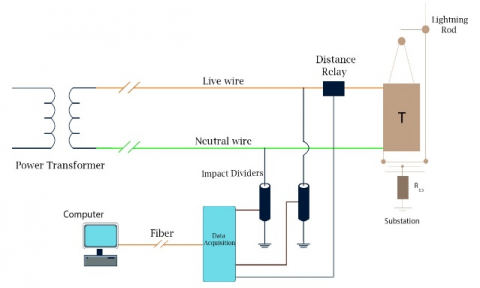
5.1 SCADA interface block diagram
Our idea is to monitor the two-port network of the Transmission line system by using SCADA, this helps in monitoring the system and to identify the faults and we can also record the data regarding the faults occurred in the system.
Figure 15. SCADA interface diagram
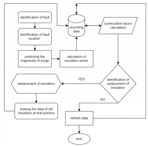
Figure 16. Algorithm of the proposed idea
The new methodology as shown in Figure 15 deals with the identification of fault location using distance relay in order to use in future analysis purpose. we must identify the fault parameters and analyze the electrical stress encountered by the insulation at the position of fault. We have to employee a long-range distance relay in between the power transformer of the generating station and primary distribution station to analyze The UHV lines. We have built an algorithm shown in Figure 16, which identifies the places where more faults occurred and we have to calculate the electrical stress on the insulation installed at that particular place based on the previous data recorded. SDFL (Smart-dispatching Decision-support and Fault Location) is an advanced application system based on EMS (Energy Management System), GIS (Geographic Information System) and fault recorder system. It is mainly used to judge the nature of power grid faults and locate faults. But the algorithm presented in this paper uses the simple data given by the distance relay and there is no need of GIS as we go with the numbering of poles. This helps in identifying the insulation strength by which we can predict the survival of that insulation in further fault cases and analyze if replacement is needed or not in order to reduce the probability of lightning outage and insulation failure at the time of lightning strike, this helps introducing the faults entering into the phase Wires of the transmission line.
In order to record and save the data in the server we use SCADA system and we employee certain communication systems in order to achieve the required conditions. The data cables which come from the distance relay are given to the RTU (remote terminal unit) just as the IED (Intelligence Electronic Device) and this data communication is taken place. The recorded data must be made available to the compiler which runs the code to calculate the dielectric strength of the insulation in the transmission lines. The lifetime of the insulation is affected by various factors such as treeing, tracking, Electrical stress on insulation.
The lifetime of insulation is directly proportional to the electric field intensity.
L = E-n K (88)
where, K is a constant.
In order to find the ageing, we have to identify the lifetime of insulation for the surge parameters and predict the ageing of the insulation.
Let us consider two surge conditions for the detailed study.
Step 1: Identification of fault location.
Table 1. Surge location
|
Surge location |
Insulation point 1 |
Insulation point 2 |
|
787m |
INS26 |
INS27 |
Table 1 represents that the fault occurred at 787 meters is in between the Pole insulation INS26 and INS27. INS is the naming of insulation and the number represents the transmission line poles that cover the fault.
Step 2: Identification of surge parameters and aging calculation.
Table 2. Surge parameters
|
Surge parameters |
Case 1 787m |
Case 2 1327m |
|
Surge voltage magnitude |
3.5MV |
1MV |
|
Back flashover |
Yes |
No |
|
Lightning shielding |
Fail |
Success |
|
electrical stress |
High |
Moderate |
|
Insulation ageing factor |
0.7 |
0.2 |
The ageing factor represents the lifetime reduction and as we can see from the Table 2, the ageing of insulation is faster in case 1 when compare to the case 2. This implies about the change of insulation requirement. By this method we can pre determine if any insulation is going to fail or age early than assumed time.
5.2 Communication system
The communication systems are connected to the RTU of the substation. so, we are going to place the distance relay near to the sub-station and the RTU of the primary distribution sub-station will accept the data regarding the distance relay. The data is also collected from the impact dividers which provide more detailed information regarding the surges generated, but mostly impact dividers are reliable when there is a short transmission path. A distance relay can be considered after the generating station with a long range so that tracking the faults will become easy and efficient. The communication is done mostly in two ways, which are mentioned below:
Both the MPLS and GPRS, the data is transferred in the form of packets.
A. MPLS: In this communication system, the output of the RTU is given to the MPLS with FO (Fiber Optic) cables. This sends the data to the control center. It adds a MPLS label to the data which allows the IP packets of the data to pass at switching level, without being passed up to the routing level, by which the transmission is done faster when compared to the packet data transfer.
B. GPRS: This is the secondary option for communication, where the Router will be installed with a SIM card and it transmits the signal through 3G network in case of FO breakdown condition. This data gets transmits through the MPLS communication system.
5.3 Working of MPLS
IP address of data before MPLS label.
In routing level, the IP of the data is checked at each stage of transmission through router.
Now, the routers only look at the MPLS label, and never check the IP address till the receiver level. This label creates a pre-defined path to the data from transmitter to the receiver, which makes the data to travel faster when compared to routing level. MPLS creates an end-to-end path that act like a circuit switched condition. Since layer-3: routing function is made to act like layer-2: switching function the MPLS is also called as 2.5-layer protocol.
5.4 Future scope of the integration with SCADA
In future this system can also include the weather forecast details which helps in increasing the efficacy in identification of insulation ageing factor as it has a collective data of electrical and environmental stress applied over the insulation which helps in the in-depth analysis of condition of insulation.
In order to attain high lightning shielding success, insulation is critical. As a result, determining the insulation strength in advance based on common problems aids in tracking the insulation's ageing rate. The RBF is employed in addition to FDTD to provide accurate surge magnitude estimates, which were further used to compute the insulation factor. We have devised a new element called Insulation Ageing Factor, which aids in determining insulation ageing based on previous data of the insulation stored in database.
[1] Liu, Z. (2015). Chapter 5 - Lightning overvoltage and protection of UHV grid. Ultra-High Voltage Ac/dc Grids, pp. 193-227. https://doi.org/10.1016/B978-0-12-802161-3.00005-6
[2] Vu, L.A.P., Vu, P.T. (2012). Calculation of lightning-induced voltages on overhead power lines using the RBF-FDTD method. In 2012 10th International Power & Energy Conference (IPEC), pp. 573-577. https://doi.org/10.1109/ASSCC.2012.6523331
[3] Williams, T. (2017). Chapter 16 - Systems EMC. EMC for Product Designers (Fifth Edition), pp. 457-484.
[4] Fan, C.L., Wu, G.N., Li, R.F. (2008). Study on shielding failure flashover rate for EHV transmission line. In 2008 International Conference on High Voltage Engineering and Application, pp. 172-175. https://doi.org/10.1109/ICHVE.2008.4773901
[5] Geng, J., Jia, B.Y., Gao, S.G. (2012). Calculation of lightning outage rate of high voltage transmission line. In 2012 Asia-Pacific Power and Energy Engineering Conference, pp. 1-4. https://doi.org/10.1109/APPEEC.2012.6307346
[6] Rizk, M.E., Mahmood, F., Lehtonen, M., Badran, E.A., Abdel-Rahman, M.H. (2016). Computation of peak lightning-induced voltages due to the typical first and subsequent strokes considering high ground resistivity. IEEE Transactions on Power Delivery, 32(4): 1861-1871. https://doi.org/10.1109/TPWRD.2016.2555856
[7] Rizk, M.E., Mahmood, F., Lehtonen, M., Badran, E.A., Abdel-Rahman, M.H. (2016). Influence of highly resistive ground parameters on lightning-induced over voltages using 3-D FDTD method. IEEE Transactions on Electromagnetic Compatibility, 58(3): 792-800. https://doi.org/10.1109/TEMC.2016.2527503
[8] Bullich-Massague, E., Sumper, A., Villafafila-Robles, R., Rull-Duran, J. (2014). Optimization of surge arrester locations in overhead distribution networks. IEEE Transactions on Power Delivery, 30(2): 674-683. https://doi.org/10.1109/TPWRD.2014.2312077
[9] Mahmood, F., Sabiha, N.A., Lehtonen, M. (2015). Probabilistic risk assessment of MV insulator flashover under combined AC and lightning-induced over voltages. IEEE Transactions on Power Delivery, 30(4): 1880-1888. https://doi.org/10.1109/TPWRD.2015.2388634
[10] Takami, J., Okabe, S., Zaima, E. (2009). Study of lightning surge over voltages at substations due to direct lightning strokes to phase conductors. IEEE Transactions on Power Delivery, 25(1): 425-433. https://doi.org/10.1109/TPWRD.2009.2033975
[11] Napolitano, F. (2010). An analytical formulation of the electromagnetic field generated by lightning return strokes. IEEE Transactions on Electromagnetic Compatibility, 53(1): 108-113. https://doi.org/10.1109/TEMC.2010.2065810
[12] Paolone, M., Rachidi, F., Borghetti, A., Nucci, C.A., Rubinstein, M., Rakov, V.A., Uman, M.A. (2009). Lightning electromagnetic field coupling to overhead lines: Theory, numerical simulations, and experimental validation. IEEE Transactions on Electromagnetic Compatibility, 51(3): 532-547. https://doi.org/10.1109/TEMC.2009.2025958
[13] Araujo, A.E., Paulino, J.O., Silva, J.P., Dommel, H.W. (2001). Calculation of lightning-induced voltages with RUSCK's method in EMTP: Part I: Comparison with measurements and Agrawal's coupling model. Electric Power Systems Research, 60(1): 49-54. https://doi.org/10.1016/S0378-7796(01)00167-5
[14] Vu, A.P.L., Vu, T.N.P., Huynh, T.N., Vu, T.P. (2016). The RBF-FDTD method for modeling the lightning-induced voltages on overhead distribution lines. Science and Technology Development Journal, 19(2): 25-33. https://doi.org/10.32508/stdj.v19i2.644
[15] Andreotti, A., Assante, D., Mottola, F., Verolino, L. (2009). An exact closed-form solution for lightning-induced over voltages calculations. IEEE Transactions on Power Delivery, 24(3): 1328-1343. https://doi.org/10.1109/TPWRD.2008.2005395
[16] Zygiridis, T.T., Tsiboukis, T.D. (2004). Low-dispersion algorithms based on the higher order (2, 4) FDTD method. IEEE Transactions on Microwave Theory and Techniques, 52(4): 1321-1327. https://doi.org/10.1109/TMTT.2004.825695
[17] Sponsor. (2013). IEEE guide for direct lightning stroke shielding of substations. IEEE Std 998-2012 (Revision of IEEE Std 998-1996), pp. 1-227. https://doi.org/10.1109/IEEESTD.1996.81546
[18] Cooray, V., Scuka, V. (1998). Lightning-induced over voltages in power lines: Validity of various approximations made in overvoltage calculations. IEEE Transactions on Electromagnetic Compatibility, 40(4): 355-363. https://doi.org/10.1109/15.736222