Henri-Joël Akoue* | Pascal Ntsama Eloundou | Salomé Ndjakomo Essiane | Pierre Ele | Léandre Nneme Nneme | Benjamin Salomon Diboma | Olivier Thierry Sosso Mayi
© 2021 IIETA. This article is published by IIETA and is licensed under the CC BY 4.0 license (http://creativecommons.org/licenses/by/4.0/).
OPEN ACCESS
In this paper, we propose a novel hybrid algorithm based on MAX-MIN Ant System version of ant colony optimization coupled with quadratic programming (MMAS-QP). Quadratic programming is used to optimize the Economic Dispatching process and MMAS for planning the switching schedule of a set of production units. The algorithm is implemented in MATLAB software environment for two systems, one is 4 generating units running for 8 hours, and the other is 10 generating units running for 24 hours. The impact of heuristic parameters on the behavior of the algorithm is highlighted through the parameters setting. Results obtained shows improved solution compared to several methods such as Modified Ant Colony Optimization (MACO), particle Swarm Optimization combined with Lagrange Relaxation (PSO-LR), Swarm and Evolutionary Computation (SEC), Particle Swarm Optimization combined with Genetic Algorithm (PSO-GA). The proposed method improves sufficiently the quality of the solution as well as the execution time.
heuristic algorithms, hybrid algorithm, MAX-MIN ant system, metaheuristic, quadratic programming, unit commitment
Unit commitment problem (UCP) is a combinatorial optimization problem that consists of planning the switching schedule of a set of production units [1-3]. Moreover, UCP allows us to determine over a precise planning period the power that each unit should produce in order to meet energy demand while respecting the economic or environmental constraints imposed [4]. UCP is therefore a complex problem that involves both binary variables and continuous variables and for which several solutions are proposed in the literature. UCP was proposed for the first time by Lowery in 1966. The dynamic programming method was used to overcome the major difficulty of enumerative methods. Indeed, the enumerative methods consists in testing all possible combinations of supply with the units considered in order to choose the optimal solution. This procedure may require significant resources for a large number of units.
Nevertheless, various methods have been used to solve the UCP. Amongst these methods are the Lagrangian method [5], Tabu search [6], Neural network [7], Fuzzy logic [8], Corridors of observations method [9], Particle swarm optimization [10], Artificial bee colony algorithm [11], and Ant colony algorithm [12]. Ant Colony optimization algorithm is a metaheuristic method which was introduced by Dorigo et al. in 1991 [13]. This method is inspired by the behavior of ant when searching their food. This algorithm is focused on artificial ants building their solutions in a given optimization problem and exchanging the quality of their solutions by a mechanism inspired from the behavior of real ants [14]. Even if their major drawback its slowness of convergence, in particular when solving large scale problems, Ant Colony algorithms is widely used for their great flexibility due to their distributed and adaptive nature [1]. This nature gives them average performance in the static case, but seem more suited for dynamic problems.
The first and original version of ACO called Ant system (AS) was applied for the first time to solve the traveler salesman problem [13, 15]. Unfortunately, the results obtained while using the original version of the AS were not competitive compared to those solutions from other algorithms such as GA, PSO [1]. As matter of fact, several improved versions were developed such as the ACS (Ant Colony System) version [16], MMAS (MAX-MIN Ant System) version [17]. In fact, AS algorithm follows proportional random transition rule [18]; the pheromone is deposited and evaporated in each path proportionally to the length of the path. Ant colony System (ACS) [16] version use a pseudo-random transition rule and the pheromone are deposited and evaporated only on best solutions [18]. MAX-MIN Ant System (MMAS) [19] is an improved version of AS developed by Stützle and applied to solve few optimization problem [19, 20].
Several studies have proposed MMAS approaches to solve some problems. Stützle et al. [20] proposes an extension of MAX-MIN Ant System and apply it to Traveling Salesman Problems and Quadratic Assignment Problems. He made two main changes, namely the modification of the transition rule and the addition of a local search method. The proposed version presents better results than the ACS and MMAS algorithms. Otherwise, the obtained results show that this algorithm can be used to efficiently find near-optimal solutions to hard combinatorial optimization problems and that it is one of the best methods for solving structured quadratic assignment problems.
Zecchin et al. proposes in 2003 [21] a method for optimizing a water distribution system using the MMAS algorithm. The proposed algorithm was tested on two systems of different sizes and the results were compared with those obtained with Ant System and the Genetic Algorithm. For the first system, the developed MMAS algorithm produced better results in terms of costs and computation time than the AS and GA algorithms [21]. For the second system, even if the proposed algorithm could not lead to the optimal solution, there is however a significant reduction in the computation time compared to the GA algorithms which provided a better cost.
Bai et al. in 2009 implements a parallel version of the MMAS algorithm on GPUs with a CUDA architecture [22]. The algorithm was tested on the traveling salesman problem and the results were compared to a sequential version of MMAS. The results show that the parallel version reduces solution costs and improves computational speed by a factor greater than 2 for different size of problem.
Santos et al. in 2016 applied the MMAS algorithm to the path planning problem for a mobile autonomous robot [23]. The compared results pointed that the MMAS algorithm was more efficient for this task than GA. Moreover, MMAS was able to find the optimal solution for all the topological maps tested.
Al-Shihabi et al. propose in 2017 a method of solving the financial planning problem based on the MMAS algorithm [24]. Three versions of MMAS using different heuristic functions during solution generation have been implemented and tested on 60 sample problems. The results obtained have been compared with those produced with Branch and Bound approaches (BB) and show that MMAS allows the lowest computation time.
Yu et al. developed in 2010 a hybrid approach for solving the unit commitment problem based on the MMAS version of ACO and the lambda iteration method [25]. Here, the lambda iteration method is used to determine economic dispatching and MMAS to determine the on/off schedule for the units over the planning period. This method was simulated in the MATLAB environment on 4 systems of different sizes. In order to improve the computation efficiency, the solution of unit commitment is coded into unit operation sequence, making the space complexity fall. The results obtained demonstrated the efficiency of this method and that its more suitable than the Genetic Algorithm (GA), Evolutionary Programming (EP) and Priorty List (PL) algorithms.
Lai et al. in 2012 [26] implements an MMAS version of ACO and an improved version by adding a local update process suitable for the UCP. Both versions were tested on a 10-unit system over a running period of 24-hour horizon and the results obtained are better than those obtained by the Hybrid Particle Swarm Optimization (HPSO), GA, Here-And-Now (HN) approach and the classic version of the ACO.
Taking into consideration the advantages of the MMAS algorithm previously highlighted, several authors have exploited this method for solving optimization problems such as Traveling Salesman [22], optimization of water distribution system [21], path planning [23], financial planning [24], and unit commitment [26]. MMAS (Max-Min Ant System) has the capacity of avoiding stagnation while others versions fail to it. Furthermore, the pheromone is bounded between a minimal value $\tau^{\min }$ and a maximal value $\tau^{\max }$. With the MMAS, only best ants are allowed to update the pheromone in their path, thus this yield to best solutions found in each iteration of algorithm. The drawbacks of Ant colony algorithm in general are that probability distribution change by iteration, time to convergence is uncertain (but convergence is guaranteed), research is experimental rather than theorical [1, 27]. These weaknesses of the MMAS could be strengthen by combining it with quadratic programming.
Quadratic programming is one of the most successful approaches for solving nonlinearly constrained optimization problems since its popularization in the late 1970s.This method has been used sole or combined with others algorithms (hybridization) in the literature by several authors and has produced satisfactory and very encouraging results for a wide variety of problems. Among these problems, we have electrical power management problems as the economic load dispatch [28], optimal power flow [29] and unit commitment [30].
This paper proposes of course a new hybrid Ant Colony algorithm for solving the unit commitment problem combining MMAS algorithm and Quadratic programming.
In this hybridization Quadratic programming method is used to optimize economic load dispatch (ELD) and the on/off switching program of units is ensured by MMAS algorithm.
The rest of the paper is organized as follows: Following the introduction, section 2 presents the mathematical formulation of unit commitment problem. Section 3 describe the keys steps of MMAS algorithm. Section 4 focusses on the proposed hybrid method for solving UCP. MAX-MIN Ant system algorithm and Quadratic programming method are developed. Section 5 clarify the setting of the initial heuristic parameters. Then section 6 is devoted to the presentation of the results and section 7 offers a conclusion.
Unit commitment problem is an optimization problem whose aim is to minimize the production cost by committing available units within their constraints taken over a period. The total production cost is the sum of the production cost, the startup cost and shut down cost of all the committed units. Thus, the formulation of UCP involves the objective function and various constraints. In this study, we consider a Thermal formulation approach by considering the production cost as the only optimization criterion. The production cost therefore comprises three terms: the fuel cost, the start-up cost and the shutdown cost.
2.1 Objective function
The objective function unit commitment problem is expressed as:
$\min \left(\sum_{i=1}^{N} \sum_{t=1}^{T}\left(F_{i}\left(P_{i}(t)\right) U_{i}(t)+S T_{i}(t) U_{i}(t)+S D_{i}(1\right.\right. \left.\left.\left.-U_{i}(t)\right) U_{i}(t-1)\right)\right)$ (1)
where,
$F_{i}\left(P_{i}(t)\right)=a_{i}+b_{j} \cdot P_{i}(t)+c_{i} \cdot P_{i}(t)^{2}$ (2)
$S T_{i}(t)=\left\{\begin{array}{c}H S C_{i}, \text { si } T_{\min , i}^{\text {off }} \leq T_{i}^{\text {off }} \leq T_{\min , i}^{\text {of }}+S C_{i} \\ C S C_{i}, \text { si } T_{i}^{\text {off }}>T_{\min . i}^{\text {off }}+S C_{i}\end{array}\right.$ (3)
$i$ is the unit identification number; $N$ is the total number of units; $T$ denotes the period of scheduling; $F_{i}\left(P_{i}(t)\right)$ is the fuel cost of the unit $i$ at the time $t$ when the unit generates a power $P_{i}(t) ; U_{i}(t)$ represent the status of unit $i$ at the time $t$; $S T_{i}(t)$ et $S D_{i}\left(1-U_{i}(t)\right)$ are respectively the startup and shut down cost of unit $i$ at the time $t ; a_{i}, b_{i}$ and $c_{i}$ are fuel costs coefficient of unit $i$.
$T_{\min , i}^{o f f}$ is the minimum down time of unit $i ; S C_{i}$ is the number of cold-start hours of unit $i$;
$H S C_{i}$ and $C S C_{i}$ are respectively the hot startup cost and cold startup cost of unit $i$.
2.2 Constraints
We present here the four constraints which accompany the minimization of the objective function. These four constraints are: the load demand constraints, the constraints related to spinning reserve, the constraints relating to the production limits of each unit, and the constraints relating to minimum up and minimum down time of each unit.
2.2.1 Load demand constraints
In an electrical energy supply system, production must constantly balance demand. If we consider that losses energy is not involved here, we have:
$\sum_{i=1}^{N} U_{i}(t) p_{i}(t)=D_{t}, t \in\{1, \ldots \ldots, T\}$ (4)
$D_{t}$ represents the load demand at the time t.
2.2.2 Constraints related to spinning reserve
Any sudden drops in production can be observed while supplying the load. This can happen by prediction deviation in a real-time supply or even during a failure of one or more production units in operation [31]. Besides, a way to minimize such effects and to balance the losses quickly, it is necessary to provide spinning reserve for the demand load at that time. This can be achieved by taking into account the spinning reserve $R_{t}$ in the balance equation of load demand constraints.
$\sum_{i=1}^{N} U_{i}(t) p_{i}(t) \geq R_{t}+D_{t}, t \in\{1, \ldots \ldots, T\}$ (5)
2.2.3 Constraints relating to the production limits of each unit
Due to the characteristics of each generating unit i the generated power is bounded by two limits, the lower limits denoted $\operatorname{Pmin}_{i}$ and the upper limit $\operatorname{Pmax}_{i}$. Thus, we have:
$P \min _{i} \leq p_{i}(t) \leq P \max _{i} . U_{i}(t), t \in\{1, \ldots \ldots, T\}$ (6)
2.2.4 Constraints relating to minimum up and minimum down time of each unit
The minimum start-up time is the time after which a unit can be stopped after it has been started. Likewise, the minimum shutdown time is the time after which a unit can reliably be considered shutdown and stable for a possible restart. These conditions are achieved by:
$T_{i}^{\text {on }} \geq T_{i}^{\text {up }}$ and $T_{i}^{\text {off }} \geq T_{i}^{\text {down }}$ (7)
where, $T_{i}^{u p}$ and $T_{i}^{\text {down }}$ are respectively the minimum up time and the minimum down time of the unit $i$.
MAX-MIN Ant System algorithm has been defined and used by some authors for solving a number of problems. This is the case in the ref. [24] for financial planning problem and for path planning problem in the ref. [23]. In this work, MAX-MIN Ant system is used to solve the unit commitment problem. The approach adopted is that the trials limits values are calculated for each period and we use a pheromone matrix for each time transition. This means that we are using N pheromone matrices for a horizon of N hours. Let us recall here the transition rule and the pheromone update rule of MMAS.
3.1 MMAS state transition rule
In the MMAS algorithm, ants build a solution in a probabilistic way step by step by using information related to pheromone and specifics heuristics information of the given problem. Thus, the probability for an ant k to moves from state i to the state j, is given by Eq. (8).
$P_{i, j}^{k}=\frac{\tau_{i, j}^{\alpha} \cdot \eta_{i, j}^{\beta}}{\sum_{k=1}^{c} \tau_{i, k}^{\alpha} \cdot \eta_{i, k}^{\beta}}$ (8)
with α, β: are respectively the relative importance of intensity and visibility.
$\eta_{i, j}$ : Visibility of the solution.
$\tau_{i j}:$ Pheromone intensity of the path.
3.2 MMAS pheromone updating rule
The pheromone update is done after each iteration. The update rule in each path is given by Eq. (9).
$\left\{\begin{array}{c}\tau_{i, j} \leftarrow(1-\rho) \cdot \tau_{i, j}+\Delta \tau_{i, j}^{\text {best }} \text { if } \tau^{\min }<\tau_{i, j}<\tau^{\max } \\ \tau_{i, j} \leftarrow \tau^{\max } \text { if } \tau_{i, j}>\tau^{\max } \\ \tau_{i, j} \leftarrow \tau^{\min } \text { if } \tau_{i, j}<\tau^{\min }\end{array}\right.$ (9)
$\Delta \tau_{i, j}^{\text {best }}$ is defined by the Eq. (10):
$\Delta \tau_{i, j}^{b e s t}=\left\{\begin{array}{c}\frac{1}{L_{b e s t}} \text { if the path }(i, j) \text { is the best } \\ \text { amongst the solution } \\ \text { 0 elsewhere. }\end{array}\right.$ (10)
where:
$\rho$ : pheromone evaporation coefficient.
$L_{\text {best }}$ : best solution cost.
Quadratic programming is used to optimize the Economic load Dispatching (ELD) process and MMAS for planning the switching schedule of a set of production units. This section describes clearly the procedure of the proposed hybrid optimization algorithm.
4.1 Quadratic programming for economic dispatching
Once the search space is established, the ELD is carried out for each state and each hour of the planning period, taking into account the characteristics of the units and that of the demand.
ELD is a sub-problem of unit commitment, which consists of production cost minimizing for each given operating moment in order to achieve the power economic dispatching between operational units.
The objective function to be minimized is expressed as follows:
$\min \left(\sum_{i=1}^{N} \sum_{t=1}^{T} F_{i}\left(P_{i}(t)\right)\right)$ (11)
where, $F_{i}\left(P_{i}(t)\right)$ is the expression of the fuel cost function of unit i in time t and given in Eq. (2).
In this paper, to solve the economic dispatching problem, quadratic programming is used. It is an optimization method for solving optimization problems whose objective function is a quadratic function with linear constraints [28, 32].
The goal of quadratic programming is to find the vector x that minimizes the quadratic function $\frac{1}{2} x^{T} H x+f^{T} x$.
Hence the expression of the following objective function:
$\min \left(\frac{1}{2} x^{T} H x+f^{\mathrm{T}} x\right)$ (12)
The minimization of this function is subject to various constraints:
-Inequality constraints
$A x \leq b$ (13)
-Equality constraints
$A_{e q} x=b_{e q}$ (14)
-Boundary constraints
$l b \leq x \leq u b$ (15)
$H, A$ and $A_{e q}$ are matrices, and $f, b, b_{e q}, l b$, and $x$ are vectors.
Note that, the quadratic programming algorithm requires equality constraints, all-inequality constraints must be converted to equalities by introducing slack variables. Thus, each quantity that is bounded by upper and lower limits introduces two constraints and two new variables [32]. However, nowadays, most solvers used for this purpose take care of this conversion.
In order to adapt the problem of economic load dispatching to the quadratic programming method, the variables of the objective function have been redefined as follows:
$x=\left[p_{1} p_{2} \ldots \ldots \ldots \ldots \ldots p_{n}\right]^{T}$ (16)
$H=2 *\left[\begin{array}{ccc}C_{1} & 0 & 0 \\ 0 & \ddots & 0 \\ 0 & 0 & C_{n}\end{array}\right]$ (17)
$f=\left[b_{1} \cdots \cdots \cdots \cdots b_{n}\right]$ (18)
In order to satisfy the equality constraint (2.17), $b_{e q}$ have been set such that:
$b_{e q}=D t$ and $A_{e q}=\left[u_{1} u_{2} \cdots \cdots u_{n}\right]$ (19)
Production ranges constraints of units are imposed on the quadratic programming solver on the form:
$-\quad l b=\left[P 1^{\min } \quad P 2^{\min } \ldots P n^{\min }\right]$ (20)
$-\quad u b=\left[\begin{array}{llll}P 1^{\max } & P 2^{\max } & \ldots & P n^{\max }\end{array}\right]$ (21)
In order to solve the problem of economic dispatching by quadratic programming, the following steps have been followed:
-Steps 1: initialize the procedure and assign the smallest value to each generator.
-Step 2: bring back H, f, Aeq, beq, lb, ub in their matrix form using expressions (16)-(21).
-Step 3: replace the quantities from step 2 in a quadratic programming solver in order to determine the optimal power to be allocated to each generator.
-Step 4: check the convergence using the relation.
$\left|D_{t}-\sum_{i=1}^{n} P_{i} U_{i}(t)\right| \leq \varepsilon$ (22)
where, ε is the tolerance for violation of the balance between generated power and the load demand.
By considering spinning reserve capacity.
$\sum_{i=1}^{n} P_{i} U_{i}(t)=D_{t}+R_{t}$
$1 \leq t \leq T i \epsilon \in \mathbb{N}^{*}$ (23)
Steps 1 to 4 are repeated until there is convergence of the algorithm.
Once the ELD is completed, at each state of each hour of the search space is now associated a combination of active/inactive units and an optimal output power.
4.2 MAX-MIN ant system-quadratic programming for unit commitment problem
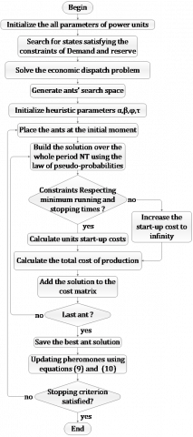
The algorithm can be divided in 6 keys steps: the initialization of the all parameters of power units, definition of search space, economic dispatching of power by using quadratic programming, initialization of heuristic parameters, exploration of search space and pheromones update.
4.2.1 Initialization of the all parameters of power units
Firstly, the parameters of the power units are initialized with the characteristics of different units for given data set. It is specified for each unit the power range, fuel cost coefficients, hot startup cost and cold startup cost, minimum up time and the minimum down time. In this part the forecasted load demands are also initialised.
4.2.2 Search space definition
After the first step, all combinations of the UCP are found in the form of binary variables by using exhaustive enumeration. Thus, for a system of n units we will have $2^{n}$ combinations. Furthermore, for each period, all state that their power cannot satisfy load and spinning reserve are eliminated; as matter of fact, the reminding state are used to build our ant search space.
Assuming that for a system of $n$ units, over a horizon of $T$ hours, if $k_{i}$ is the number of eliminated states for $i$ hour and $n_{i}=2^{n}-k_{i}$ number of states remaining, each ant examines $\prod_{i=1}^{T}\left(2^{n}-k_{i}\right)$ cases to find the minimum cost path. For high values of $n$ and $T$, this number of cases can become very important and thus lead to unsuitable computational time. In this article in order to reduce the number of states and reduce the computational time, especially for the 10 units in 24 hours system, a priority order has been set for each hour. This priority order is based on the frequency of operation of each unit at full load and on minimization of transition cost. It should be noted that for the case of 4-unit system, no reduction in the number of cases was made.
4.2.3 Economic load dispatch
Once the search space is established, quadratic programming is used to realize the ELD for each state in each period of scheduling. This is done by taking into account the characteristics of each unit, the load demand and the spinning reserve.
After the realization of ELD, for each state at any time on the search space, an optimal combination of actives/inactives of units is associated.
For a T horizon, to move from hour $i$ to hour $i+1$ we form a pheromone matrix of dimension $n_{i} \times n_{i+1}$. where $n_{i}$ and $n_{i+1}$ are the number of states for hour $i$ and $i+1$ respectively.
4.2.4 Initialisation of algorithm parameters
Appropriate parameters for the algorithm are well defined in initialization step. Out of them, we have: the number of ants (m), the relative importance of pheromone (α), the relative importance of visibility (β), the evaporation coefficient (ρ), as well as the initial, maximum and minimum quantities of pheromones on each arc respectively $\tau_{0}, \tau_{\max }$ and $\tau_{\min }$.
The quantity of deposit pheromone is given by the following relationships [19, 26]:
$\tau_{0}=\frac{1}{\sum_{t=1}^{T} \min F\left(D_{t}\right)}$ (24)
where, $\sum_{t=1}^{T} \min F\left(D_{t}\right)$ is the sum of points with the smallest generating cost in each period.
$\tau_{\max }=\frac{1}{1-\rho} \tau_{0}$ (25)
$\tau_{\min }=\frac{\tau_{\max \left(1-\sqrt[n]{\left.P_{\text {best }}\right)}\right.}}{(\operatorname{avg}-1) \sqrt[n]{P_{\text {best }}}}$ (26)
where, $P_{\text {best }}$ is the probability of finding the optimal solution when the MMAS algorithm converges, which is generally 0.05 [33].
4.2.5 Exploration of search space
In this step, each ant explores the search space looking for the best solution as possible. Every ant starts with a minimal cost in the first hour till the last hour; the transition rule is given by Eq. (8).
In each transition, constraints related to minimum up time and minimum down time are set. If these constraints are fulfilled, then startup cost are calculated, if they are not fulfilled startup cost are set to infinity.
At the last hour, the total production cost of the solution found is calculated and saved. The solution is added in the total cost matrix which the size depends on the number of units as well as the planning horizon. The total production cost takes into account the fuel costs and the startup costs. We repeat the procedure to all the ants after comparison and only the best solution is saved.
4.2.6 Pheromones update rule
This operation consists of reinforcing the pheromone tracks associated with promising solutions and, on the contrary, degrading by “evaporation” that associated with bad solutions. The pheromone update rule is given by Eq. (9).
4.2.7 MMAS-QP algorithm for solving the UCP
UCP is solved by using MMAS algorithm through the following steps:
Step 1: Initialize the all parameters of power units.
Step 2: search all state combinations on/off able to satisfy the load demand and spinning reserve.
Step 3: for each state found in step 2, find the optimal power able to satisfy load demand constraints through quadratic programming process.
Step 4: initialization of algorithm parameters.
Step 5: Exploration of search space.
ants are released randomly at an initial state in the first hour.
from the first hour till the last hour, each ant builds his solution by choosing the next state in aid of the transition rule (law of pseudo-probabilities).
When the tour is completed, we introduce the minimum up and down time constraints to check if the corresponding path fulfills the unit constraints: two case are studied:
-If the found path fulfills those unit constraints, we compute the total cost and save it.
-If it does not satisfy the constraints, then cost is set to infinity ($\infty$).
We calculate the total production cost.
Step 6: Save the minimal cost and apply update pheromone rule to each path.
If the end of criterion is achieved then print unit commitment schedule, else returned to step 5.
The Figure 1 present a flowchart that summarizes all these steps.
Figure 1. Flowchart of MMAS algorithm for UCP
The setting of initial heuristic parameters of an algorithm can have direct consequences on convergence behaviour. It is therefore necessary in this work to set heuristic parameters through criteria such as cost and speed. 2. Thus we have done manual adjustment of heuristic parameters with emphasis on the impact of each heuristic parameters on algorithm behaviour as the total generation cost and the execution time. This is one of the main contributions of this work. The settings are done on numerical for 4-unit system and 10-unit system whose generator characteristics and load demand are given in Appendix.
Apart from the $P_{\text {best }}$ and Q parameters whose values were respectively adjusted to 0.05 and 0.9 by considering the results produced in literature [33, 34] and the verification tests carried out, the other parameters are adjusted here. The parameters are adjusted by sampling and interpreting several measurements. The idea is to maintain the values of the other parameters and vary the one that the best value must be determined within the defined interval. The advantage of this method is to extract the best values of the parameters at the same time as we study their impact on the performance of the algorithm.
For each parameter, the simulations were repeated 30 times. The desired parameters α, β, ρ, m and maxIter have been bounded as follows: 0≤α≤5; 0≤β≤87; 0<ρ<1; 0<m≤1100; 0<maxIter≤1000 for 10-unit system and 0≤α≤5; 0≤β≤25; 0<ρ<1; 0<m≤1100; 0<maxIter≤1000 for 4-unit system.
where:
α: relative importance of the pheromone trail.
β: relative importance of the visibility.
ρ: pheromone evaporation coefficient.
m: number of ants.
maxIter: maximum number of iterations.
This section records some measurements that can justify the choice made for the values of heuristic parameters respectively for 4-unit system and 10-unit system.
Even if all the statistics do not appear, it should be noted that the choice of the values of the parameters takes into account a compromise between the values of the Total average generation cost, the best costs, the worst costs and the execution time for a given number of iterations.
5.1 Choice of the ρ parameter
This part deals with choosing an optimal value for the $\rho$ parameter. The fixed initial parameters are m=50; α=0.8; β=30; maxIter=70 for 10-unit system and m=200; α=0.3; β=0; maxIter=100 for 4-unit system.
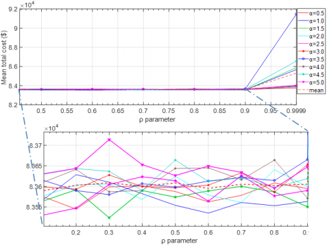
Figure 2 shows the evolution of average total generation cost as function of $\rho$ for $\alpha$ values ranging from 0.5 to 5. It appears that the production cost function diverges for values of rho greater than 0.9. For this reason, only the values of rho lower than 0.9 will be considered in the rest of this paper.
As shown in Table 1 and Table 2, a statistical treatment of the different values makes it possible to choose as the optimal value of ρ=0.3 for 4-unit system, and ρ=0.7 for 10-unit system. It should be noted that this parameter does not have significant influence on the execution time.
Figure 2. Average total generation cost as function of ρ parameter for some values of α
Table 1. Impact of the ρ parameter for 4-unit system
|
ρ |
0 |
0.1 |
0.2 |
0.3 |
0.4 |
0.5 |
0.6 |
0.7 |
0.8 |
0.9 |
|
|
TGC($) |
Best |
73444.68 |
73444.68 |
73513.87 |
73444.68 |
73444.68 |
73444.68 |
73444.68 |
73513.87 |
73444.68 |
73444.68 |
|
Average |
73869.94 |
73834.38 |
73869.18 |
73823.09 |
73889.04 |
73905.04 |
73860.19 |
73885.97 |
73876.67 |
73866.76 |
|
|
Worst |
74173.59 |
74249.13 |
74296.14 |
74166.94 |
74242.60 |
74242.72 |
74189.82 |
74184.34 |
74240.84 |
74183.12 |
|
|
Std. Deviation |
208.0237 |
214.4459 |
221.4563 |
211.7181 |
240.2445 |
227.1776 |
213.6921 |
193.7333 |
228.8980 |
218.4678 |
|
|
CV (%) |
0.2816 |
0.2904 |
0.2998 |
0.2868 |
0.3251 |
0.3074 |
0.2893 |
0.2622 |
0.3098 |
0.2958 |
|
|
Time (s) |
8.2953 |
8.2718 |
7.9408 |
7.8890 |
7.8047 |
8.1670 |
8.3258 |
8.1307 |
7.7551 |
8.3309 |
|
Table 2. Impact of the ρ parameter for 10-unit system
|
ρ |
0.1 |
0.2 |
0.3 |
0.4 |
0.5 |
0.6 |
0.7 |
0.8 |
0.9 |
|
|
TGC($) |
Best |
83522.40 |
83508.47 |
83586.62 |
83598.49 |
83664.19 |
83529.86 |
83508.47 |
83578.45 |
83578.45 |
|
Average |
83723.71 |
83706.96 |
83757.78 |
83702.63 |
83735.58 |
83702.45 |
83692.28 |
83737.57 |
83717.04 |
|
|
Worst |
83952.55 |
83860.32 |
83978.32 |
83814.48 |
83862.25 |
83926.08 |
83801.77 |
83814.48 |
83878.43 |
|
|
Std. Deviation |
121.70 |
94.49 |
127.38 |
88.19 |
59.93 |
150.22 |
95.86 |
73.03 |
94.26 |
|
|
CV(%) |
0.1454 |
0.1129 |
0.1521 |
0.1054 |
0.0716 |
0.1795 |
0.1145 |
0.0872 |
0.1126 |
|
|
Mean Time (s) |
6.69057 |
6.37258 |
6.3853 |
6.1576 |
6.1986 |
6.2872 |
6.3239 |
6.4200 |
6.3834 |
|
|
Std. Deviation |
0.0842 |
0.0925 |
0.0653 |
0.0577 |
0.0775 |
0,0796 |
0.1250 |
0,3304 |
0,1166 |
|
|
CV(%) |
1.26 |
1.45 |
1.02 |
0.94 |
1.25 |
1.26 |
1.98 |
5.15 |
1.83 |
|
TGC: Total Generation Cost
5.2 Choice of the α parameter
For this part, the fixed initial parameters are:
ρ=0.3; m=100; β=5; maxIter=50 for 4-unit system and ρ=0.7; m=50; β=30; maxIter=70 for 10-unit system and 4-unit system. Table 3 and Table 4 shows the influence of the α parameter on Mean total generation cost and mean execution time respectively for 4-unit system and 10-unit system. Table 3 shows an increasing of average total generation cost with a relatively constant execution time. It appears that α=0 present the best results for 4-unit system. Table 4 shows that for 10-unit system, the best value for α is 1.5 with a best total generation cost and good coefficients of variation for cost and execution time. It should be noted, as in the case of ρ, that the α parameter do not have a significant influence on the computation time.
Table 3. Impact of α parameter for 4-unit system
|
|
Total generation Cost ($) |
Mean Execution Time (s) |
||||||||
|
α |
Best |
Average |
Worst |
Std. Deviation |
CV(%) |
Best |
average |
Worst |
Std. Deviation |
CV(%) |
|
0 |
73444.68 |
73837.86 |
74180.31 |
215.77 |
0.29 |
6.52 |
6.66 |
7.80 |
0.57 |
8.62 |
|
0.1 |
73513.87 |
73845.68 |
73958.81 |
188.82 |
0.25 |
6.69 |
7.40 |
7.46 |
0.35 |
4.70 |
|
0.2 |
73513.87 |
73897.22 |
74171.65 |
269.76 |
0.36 |
7.36 |
8.14 |
8.30 |
0.41 |
5.01 |
|
0.3 |
73444.68 |
73861.06 |
74160.43 |
293.50 |
0.40 |
7.32 |
7.74 |
8.38 |
0.44 |
5.66 |
|
0.4 |
73794.08 |
73962.99 |
74160.43 |
149.71 |
0.20 |
7.31 |
7.78 |
8.12 |
0.33 |
4.25 |
|
0.5 |
73444.68 |
73856.84 |
74196.62 |
235.10 |
0.32 |
6.67 |
6.72 |
7.69 |
0.39 |
5.53 |
|
1 |
73513.87 |
73850.20 |
74210.34 |
215.69 |
0.29 |
6.37 |
6.61 |
7.73 |
0.37 |
5.67 |
|
1.5 |
73444.68 |
73859.25 |
74212.64 |
255.78 |
0.35 |
6.67 |
6.98 |
7.87 |
0.34 |
4.91 |
|
2 |
73513.87 |
73882.02 |
74242.72 |
220.69 |
0.30 |
6.51 |
7.01 |
7.70 |
0.41 |
5.85 |
|
2.5 |
73513.87 |
73884.74 |
74183.13 |
211.88 |
0.29 |
6.73 |
7.18 |
7.72 |
0.32 |
4.52 |
|
3 |
73444.68 |
73922.80 |
74240.84 |
218.24 |
0.29 |
6.77 |
7.30 |
7.95 |
0.38 |
5.26 |
|
3.5 |
73444.68 |
73849.36 |
74249.14 |
230.55 |
0.31 |
6.96 |
7.39 |
8.00 |
0.27 |
3.67 |
|
4 |
73444.68 |
73843.15 |
74184.34 |
230.31 |
0.31 |
7.04 |
7.82 |
8.69 |
0.66 |
8.40 |
|
4.5 |
73444.68 |
73902.53 |
74296.14 |
238.18 |
0.32 |
7.00 |
7.93 |
9.25 |
0.81 |
10.23 |
|
5 |
73444.68 |
73852.09 |
74191.56 |
243.59 |
0.33 |
7.05 |
7.32 |
8.31 |
0.42 |
5.71 |
Table 4. Impact of α parameter for 10-unit system
|
|
|
Total generation Cost (\$) |
Mean Execution Time (s) |
|||||||
|
α |
Best |
Average |
Worst |
Std. Deviation |
CV(%) |
Best |
average |
Worst |
Std. Deviation |
CV(%) |
|
0.5 |
83544.81 |
83583.60 |
83608.68 |
19.34 |
0.00023 |
3.35 |
3.45 |
3.57 |
0.08 |
0.024 |
|
1 |
83535.25 |
83572.85 |
83628.61 |
27.90 |
0.00033 |
3.32 |
3.42 |
3.56 |
0.07 |
0.020 |
|
1.5 |
83523.92 |
83574.53 |
83600.10 |
23.10 |
0.00028 |
3.42 |
3.50 |
3.61 |
0.05 |
0.015 |
|
2 |
83560.88 |
83595.36 |
83640.87 |
25.05 |
0.00030 |
3.30 |
3.41 |
3.60 |
0.09 |
0.028 |
|
2.5 |
83530.30 |
83586.44 |
83626.59 |
32.24 |
0.00038 |
3.41 |
3.54 |
3.72 |
0.13 |
0.037 |
|
3 |
83586.34 |
83610.28 |
83653.27 |
21.10 |
0.00025 |
3.40 |
3.47 |
3.65 |
0.09 |
0.025 |
|
3.5 |
83580.14 |
83611.65 |
83665.33 |
22.80 |
0.00028 |
3.43 |
3.51 |
3.71 |
0.08 |
0.024 |
|
4 |
83571.24 |
83618.81 |
83664.08 |
29.92 |
0.00036 |
3.37 |
3.47 |
3.66 |
0.10 |
0.028 |
|
4.5 |
83590.25 |
83623.72 |
83664.17 |
21.63 |
0.00026 |
3.39 |
3.52 |
3.70 |
0.10 |
0.030 |
|
5 |
83595.61 |
83643.85 |
83713.91 |
29.67 |
0.00035 |
3.39 |
3.50 |
3.72 |
0.12 |
0.033 |
5.3 Choice of the β parameter
For this part, the fixed initial parameters are ρ=0.3 α=0; m=100; maxIter=50 for 4-unit system and ρ=0.7; α=1.5; m=100; maxIter=20 for 10-unit system.
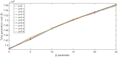
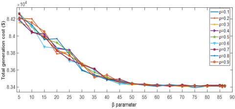
Figure 3 and Figure 4, and Tables 5 and 6 shows the total generation cost as well as the average execution time as a function of β parameters.
For ρ varying from 0.1 to 0.9, we obtain in figure 3 and figure 4 the curves that shows the evolution of the average total generation cost as a function of β. For the 4-unit system, β values are considered in the interval 0 to 25 and for 10-unit system are considered in the interval 5 to 87. Figure 3 shows for 4-unit system that the total generation cost increases significantly with increasing of β. For 10-unit system, as show in Figure 4, the total generation cost decreases with increasing of β and converge. The details given by the associated statistical study are recorded in the Tables 5 and 6. It therefore appears that the increase and decrease in β respectively for 4-unit system and 10-unit system improves the Total generation cost without degradation of time. The chosen β value is 0 for 4-unit system and 86 for 10-unit system, given the fact that they present best results.
5.4 Choice of the number of ants
The fixed initial parameters are ρ=0.3; α=0; β=0; maxIter=50 for 4-unit system and ρ=0.7; α=1.5; β=86; maxIter=20 for 10-unit system.
Tables 7 and 8 give the total generation cost and iteration time according to the number of ants. By varying the number of ants from 50 to 1100 for 4-unit system and from 10 to 1100 for 10-unit system, it appears that this parameter significantly improves the total generation cost. However, the major drawback remains the increase of execution time. It is therefore appropriate, depending on the needs, to make a good choice of m. In this paper, the choice of m is made so that we have a reduced cost and a short time as far as possible. Taking this into account the values of m chosen are 200 for 4-unit system and 300 for 10-unit system.
Figure 3. Average total generation cost as function of β parameter for 4-unit system
Figure 4. Average total generation cost as a function of β parameter
Table 5. Impact of β parameter on Total Generation cost and mean iteration time for 4-unit system
|
β |
0 |
0.1 |
0.2 |
0.3 |
0.4 |
0.5 |
0.6 |
|
|
TGC($) |
Best |
73444.68 |
73444.68 |
73444.68 |
73444.68 |
73534.46 |
73444.68 |
73816,98 |
|
Average |
73458.52 |
73836.75 |
73790.09 |
73728.81 |
73998.83 |
73833.31 |
73951.51 |
|
|
Worst |
73513.87 |
74184.55 |
73958.81 |
73959.63 |
74204.93 |
74160.43 |
74160.07 |
|
|
Std. Deviation |
27.67 |
233.93 |
130.29 |
203.27 |
215.00 |
200.09 |
126.35 |
|
|
CV (%) |
0.04 |
0.32 |
0.18 |
0.27 |
0.29 |
0.27 |
0.17 |
|
|
Time (s) |
7.23 |
7.41 |
7.44 |
7.37 |
7.37 |
7.14 |
7.26 |
|
|
β |
5 |
10 |
15 |
20 |
25 |
|||
|
TGC($) |
Best |
73444.68 |
73886.38 |
74086.69 |
74610.76 |
74794.31 |
||
|
Average |
73638.07 |
74090.02 |
74534.65 |
74746.22 |
75057.12 |
|||
|
Worst |
73842.16 |
74242.60 |
74715.36 |
74796.93 |
75165.09 |
|||
|
Std. Deviation |
146.15 |
129.59 |
169.97 |
51.14 |
114.23 |
|||
|
CV (%) |
0.20 |
0.17 |
0.23 |
0.07 |
0.15 |
|||
|
Time (s) |
7.33 |
7.34 |
7.38 |
7.32 |
7.32 |
|||
Table 6. Impact of β parameter on Total Generation cost and mean execution time
|
β |
5 |
10 |
15 |
20 |
25 |
30 |
35 |
40 |
|
|
TGC($) |
Best |
84157.57 |
84039.45 |
83873.90 |
83791.23 |
83708.33 |
83594.83 |
83514.36 |
83486.53 |
|
Average |
84218.05 |
84107.07 |
83987.79 |
83860.38 |
83785.94 |
83653.15 |
83570.96 |
83503.67 |
|
|
Worst |
84268.64 |
84202.36 |
84051.36 |
83968.87 |
83835.47 |
83682.97 |
83614.78 |
83542.30 |
|
|
Std. Deviation |
36.40 |
51.33 |
48.62 |
50.81 |
42.09 |
29.26 |
36.40 |
17.22 |
|
|
CV (%) |
0.043 |
0.061 |
0.058 |
0.060 |
0.050 |
0.035 |
0.043 |
0.021 |
|
|
Time (s) |
8.11 |
8.29 |
8.16 |
8.30 |
8.13 |
8.20 |
8.56 |
8.16 |
|
|
β |
45 |
50 |
55 |
60 |
65 |
70 |
75 |
80 |
|
|
TGC ($) |
Best |
83438.04 |
83425.99 |
83421.55 |
83407.51 |
83410.24 |
83406.24 |
83393.03 |
83393,03 |
|
Average |
83463.90 |
83437.52 |
83428.58 |
83419.78 |
83421.16 |
83415.43 |
83410.84 |
83411,52 |
|
|
Worst |
83493.70 |
83447.16 |
83440.15 |
83431.50 |
83430.66 |
83426.76 |
83420.30 |
83421,19 |
|
|
Std. Deviation |
16.73 |
5.85 |
5.64 |
6.38 |
5.67 |
7.29 |
7.30 |
7.59 |
|
|
CV (%) |
0.020 |
7.01E-03 |
6.76E-03 |
7.64E-03 |
6.80E-03 |
8.74E-03 |
8.76E-03 |
9.10E-03 |
|
|
Time (s) |
8.21 |
7.99 |
8.06 |
8.07 |
8.05 |
8.00 |
8.02 |
8.06 |
|
|
β |
85 |
86 |
87 |
||||||
|
TGC ($) |
Best |
83393.03 |
83393.03 |
83393.03 |
|||||
|
Average |
83412.77 |
83408.11 |
83410.16 |
||||||
|
Worst |
83420.97 |
83416.16 |
83417.19 |
||||||
|
Std. Deviation |
7.894089 |
6.94 |
6.82 |
||||||
|
CV (%) |
9.46E-03 |
8.32E-03 |
8.17E-03 |
||||||
|
Time (s) |
8.16 |
8.43 |
8.09 |
||||||
Table 7. Total generation cost and mean execution time depending of the number of ants for 4-unit system
|
Ants Number |
50 |
100 |
150 |
200 |
250 |
300 |
400 |
|
|
TGC($) |
Best |
74003.21 |
73794.08 |
73444.68 |
73444.68 |
73513.87 |
73444.68 |
73534.46 |
|
Average |
74317.70 |
74078.36 |
73828.17 |
73733.85 |
73824.16 |
73861.77 |
73782.78 |
|
|
Worst |
74729.33 |
74251.64 |
74080.39 |
74013.05 |
74011.61 |
74156.83 |
73958.81 |
|
|
Std. Deviation |
218.93 |
190.21 |
138.06 |
191.13 |
153.55 |
258.76 |
153.62 |
|
|
CV(%) |
0.29 |
0.26 |
0.19 |
0.26 |
0.21 |
0.35 |
0.21 |
|
|
Time (s) |
Best |
2.23 |
3.89 |
5.71 |
7.29 |
9.01 |
10.58 |
17.38 |
|
Average |
2.49 |
4.02 |
5.95 |
7.58 |
9.33 |
12.58 |
18.54 |
|
|
Worst |
3.20 |
4.26 |
6.38 |
7.95 |
10.71 |
15.84 |
20.63 |
|
|
Std. Deviation |
0.26 |
0.10 |
0.24 |
0.22 |
0.49 |
2.28 |
1.15 |
|
|
CV(%) |
10.59 |
2.62 |
4.03 |
2.89 |
5.26 |
18.15 |
6.21 |
|
|
Ants Number |
500 |
600 |
700 |
800 |
900 |
1000 |
1100 |
|
|
TGC ($) |
Best |
73444.68 |
73444.68 |
73513.87 |
73444.68 |
73444.68 |
73444.68 |
73444.68 |
|
Average |
73724.12 |
73599.94 |
73675.17 |
73619.36 |
73701.97 |
73563.86 |
73610.68 |
|
|
Worst |
73868.33 |
73868.33 |
73817.54 |
73879.13 |
73865.79 |
73799.14 |
73817.19 |
|
|
Std. Deviation |
148.50 |
170.57 |
146.27 |
169.25 |
155.96 |
125.48 |
173.77 |
|
|
CV(%) |
0.20 |
0.23 |
0.20 |
0.23 |
0.21 |
0.17 |
0.24 |
|
|
Time (s) |
Best |
21.89 |
25.72 |
28.83 |
29.35 |
30.24 |
33.53 |
38.26 |
|
Average |
24.06 |
28.32 |
32.70 |
34.34 |
33.09 |
35.57 |
43.31 |
|
|
Worst |
26.83 |
31.82 |
38.30 |
38.83 |
41.95 |
42.51 |
47.76 |
|
|
Std. Deviation |
1,49 |
2.00 |
3.05 |
2.72 |
4.14 |
2.80 |
3.43 |
|
|
CV(%) |
6,18 |
7.07 |
9.32 |
7.91 |
12.51 |
7.88 |
7.91 |
|
Table 8. Total generation cost and mean execution time depending of the number of ants for 10-unit system
|
Ants Number |
10 |
50 |
100 |
200 |
300 |
400 |
500 |
|
|
TGC ($) |
Best |
83450.47 |
83437.78 |
83382.93 |
83375.32 |
83371.21 |
83371.21 |
83371,21 |
|
Average |
83644.01 |
83579.68 |
83504.95 |
83489.02 |
83441.69 |
83448.74 |
83440,42 |
|
|
Worst |
83730.27 |
83686.39 |
83598.99 |
83536.31 |
83475.57 |
83499.70 |
83486,49 |
|
|
Std. Deviation |
42.83 |
73.34 |
51.749 |
52.85 |
29.16 |
32.90 |
30.67 |
|
|
CV(%) |
0.00051 |
0.00088 |
0.00062 |
0.00063 |
0.00035 |
0.00039 |
0.00037 |
|
|
Time (s) |
1.24 |
2.33 |
3.54 |
4.68 |
6.42 |
8.16 |
10.06 |
|
|
Ants Number |
600 |
700 |
800 |
900 |
1000 |
1100 |
|
|
|
TGC ($) |
Best |
83371.21 |
83371.21 |
83375.32 |
83371.21 |
83371.21 |
83371.21 |
|
|
Average |
83432.58 |
83439.07 |
83429.15 |
83422.72 |
83432.58 |
83418.03 |
||
|
Worst |
83459.18 |
83477.25 |
83460.32 |
83460.32 |
83455.08 |
83469.90 |
||
|
Std. Deviation |
25.82 |
30.88 |
23.54 |
25.74 |
24.29 |
25.17 |
||
|
CV(%) |
0.030 |
0.037 |
0.028 |
0.031 |
0.029 |
0.030 |
||
|
Time (s) |
11.61 |
13.90 |
15.32 |
17.38 |
19.10 |
20.47 |
||
Taking into account all the previous considerations, the values retained for the parameters for 4-unit system and 10-unit system are given in Table 9.
Table 9. Optimal parameters retained
|
Parameters |
4-unit system |
10-unit system |
|
β |
0 |
86 |
|
ρ |
0.3 |
0.7 |
|
α |
0 |
1.5 |
|
m |
200 |
300 |
In this section, we present the results that come out of our various simulations of proposed MAX-MIN Ant System-Quadratic programming algorithm (MMAS-QP).
Programming and simulation have been done in Matlab software environment version 9.2.0.538062 (R2017a) on a computer Intel(R) Core (TM) i5-3340M CPU @ 2.70GHz (4 CPUs), ~2.7GHz, and 8192MB of RAM. The operating system installed is Windows 10 professional 64 bits (10.0, version 19041).
The aim here is to show the performances of the algorithm.
Two different systems of data are chosen to solve unit commitment problem because they are constantly used for validating the results of this kind of problem [35–38]. We have tested system 1 composed by 4 units over a running period of 8 hours and tested the system 2 composed by 10 units over a running period of 24 hours [34, 39]. The initial parameters used are m=200, α=0, β=0, ρ=0.3, Q=0.9, Pbest=0.05 for 4-unit system and m=300, α=1.5, β=86, ρ=0.7, Q=0.9, Pbest=0.05 for the 10-unit system.
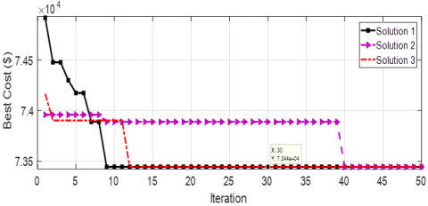
Tables 10 and 11 show the results of the units switching on/off programs, the powers generated by each generator over the planning period as well as the cumulative costs, respectively for the systems of 4 units and 10 units. We can extract from these tables the best total generation cost obtained on test system 1 for the 8 hours of the planning horizon, namely \$ 73,444.69. For test system 2 the total generation cost including the running cost of the generators and their start-up costs over the 24 hours period is \$ 83,371.2087. Answer convergence graphs are presented in Figure 5 and Figure 6 for respectively 4-unit system and 10-unit system. Three convergence graphs are given as solutions for each units system. Note that the best times to find the best solutions are 3.0155 seconds and 4.0641seconds respectively for 4 unit system and 10 unit system.
6.1 Comparison of results
Table 12 establish a comparison between the total generation costs and the computational time obtained with the proposed MMAS-QP algorithm and those obtained in the literature by other algorithms using the same system of 4-unit on 8 hours [34, 39]. The results allow to assert that the proposed algorithm significantly improves the quality of the solution with a cost difference ranging from \$488.4 to \$1787.2 (change from 0.661 to 2.376%) on 8 hours. Table 13 also compare the results of our algorithm and some others algorithms found in the literature for the 10-unit system on 24 hours. We also note that for this dataset, the algorithm shows better results than some existing algorithms for the same dataset. Thus, the difference in cost between the proposed algorithm and some others varies from $104.05 to $281.2 on 24 hours. However, [35] was able to produce a better cost generation than us. This can be justified by the fact that the reduction of the number of states to improve the computational time impacts the quality of our solution. In both Tables 12 and 13, we have recorded the different computational times despite the difference of computer specifications. This allows us to affirm that, for 4-unit system and 10-unit system our algorithm provides the best solution cost in a reasonable timeframe with one of the best times. This is certainly due to the reduction of the number of states during the economic dispatching operation and also above all to the adjustment of heuristic parameters.
Table 10. UCP Results with MMAS for 4-units system
|
Hour |
Demand (MW) |
Status of Units |
Power generated for each unit (MW) Power generations of Units (MW) |
Total Power Generated (MW) |
Fuel Cost ($) |
Transition Cost ($) |
Total cumulative Cost ($) |
|||
|
1 2 3 4 |
1 |
2 |
3 |
4 |
||||||
|
1 |
450 |
1 1 0 0 |
300 |
150 |
0 |
0 |
450 |
9109.36 |
0 |
9109.36 |
|
2 |
530 |
1 1 0 0 |
300 |
230 |
0 |
0 |
530 |
10593.04 |
0 |
19702.40 |
|
3 |
600 |
1 1 0 1 |
300 |
250 |
0 |
50 |
600 |
12412.86 |
0.02 |
32115.28 |
|
4 |
540 |
1 1 0 0 |
300 |
240 |
0 |
0 |
540 |
10782.28 |
0 |
42897.56 |
|
5 |
400 |
1 1 0 0 |
276.19 |
123.81 |
0 |
0 |
400 |
8205.79 |
0 |
51103.35 |
|
6 |
280 |
1 1 0 0 |
196.19 |
83.81 |
0 |
0 |
280 |
6067.15 |
0 |
57170.50 |
|
7 |
290 |
1 1 0 0 |
202.86 |
87.15 |
0 |
0 |
290 |
6243.83 |
0 |
63414.33 |
|
8 |
500 |
1 1 0 0 |
300 |
200 |
0 |
0 |
500 |
10030.36 |
0 |
73444.69 |
Figure 5. Answer convergence graph for 4-unit system
Figure 6. Answer convergence graph for 10-unit system
Table 11. Results provided by MMAS for UCP for 10-Units system
|
Hour |
Demand (MW) |
Power generated for each unit (MW) Power generations of Units (MW) |
Total Power Generated (MW) |
Fuel Cost ($) |
Transition Cost ($) |
Total cumulative Cost ($) |
|||||||||
|
1 |
2 |
3 |
4 |
5 |
6 |
7 |
8 |
9 |
10 |
||||||
|
1 |
1170 |
200 |
125.41 |
150 |
250 |
122.45 |
105.94 |
77.12 |
81.32 |
0 |
57.763 |
1170 |
2443.52 |
274 |
2717.52 |
|
2 |
1250 |
200 |
128.32 |
150 |
250 |
125.67 |
109.91 |
79.32 |
83.46 |
63.89 |
59.414 |
1250 |
2612.70 |
101 |
5431.23 |
|
3 |
1380 |
200 |
145.77 |
150 |
280.10 |
144.99 |
133.69 |
92.52 |
96.29 |
76.62 |
60 |
1380 |
2880.38 |
0 |
8311.61 |
|
4 |
1570 |
200 |
176.24 |
150 |
349.45 |
178.73 |
150 |
115.57 |
110 |
80 |
60 |
1570 |
3295.82 |
0 |
11607.43 |
|
5 |
1690 |
200 |
202.61 |
150 |
409.45 |
207.93 |
150 |
120 |
110 |
80 |
60 |
1690 |
3578.66 |
0 |
15186.10 |
|
6 |
1820 |
200 |
232.27 |
150 |
476.95 |
240.78 |
150 |
120 |
110 |
80 |
60 |
1820 |
3906.41 |
0 |
19092.51 |
|
7 |
1910 |
200 |
254.55 |
150 |
520 |
265.44 |
150 |
120 |
110 |
80 |
60 |
1910 |
4146.40 |
0 |
23238.92 |
|
8 |
1940 |
200 |
270.00 |
150 |
520 |
280 |
150 |
120 |
110 |
80 |
60 |
1940 |
4229.72 |
0 |
27468.63 |
|
9 |
1990 |
200 |
320.00 |
150 |
520 |
280 |
150 |
120 |
110 |
80 |
60 |
1990 |
4378.19 |
0 |
31846.82 |
|
10 |
1990 |
200 |
320.00 |
150 |
520 |
280 |
150 |
120 |
110 |
80 |
60 |
1990 |
4378.19 |
0 |
36225.01 |
|
11 |
1970 |
200 |
300.00 |
150 |
520 |
280 |
150 |
120 |
110 |
80 |
60 |
1970 |
4317.06 |
0 |
40542.07 |
|
12 |
1940 |
200 |
270.00 |
150 |
520 |
280 |
150 |
120 |
110 |
80 |
60 |
1940 |
4229.72 |
0 |
44771.79 |
|
13 |
1910 |
200 |
254.55 |
150 |
520 |
265.44 |
150 |
120 |
110 |
80 |
60 |
1910 |
4146.40 |
0 |
48918.20 |
|
14 |
1830 |
200 |
234.55 |
150 |
482.14 |
243.30 |
150 |
120 |
110 |
80 |
60 |
1830 |
3932.55 |
0 |
52850.74 |
|
15 |
1870 |
200 |
243.68 |
150 |
502.91 |
253.41 |
150 |
120 |
110 |
80 |
60 |
1870 |
4038.40 |
0 |
56889.15 |
|
16 |
1830 |
200 |
234.56 |
150 |
482.14 |
243.30 |
150 |
120 |
110 |
80 |
60 |
1830 |
3932.55 |
0 |
60821.69 |
|
17 |
1690 |
200 |
202.61 |
150 |
409.45 |
207.93 |
150 |
120 |
110 |
80 |
60 |
1690 |
3578.66 |
0 |
64400.36 |
|
18 |
1510 |
200 |
164.57 |
150 |
322.88 |
165.81 |
150 |
106.74 |
110 |
80 |
60 |
1510 |
3160.87 |
0 |
67561.23 |
|
19 |
1420 |
200 |
150.83 |
150 |
291.62 |
150.60 |
140.59 |
96.35 |
100.01 |
80 |
60 |
1420 |
2965.24 |
0 |
70526.46 |
|
20 |
1310 |
200 |
136.99 |
150 |
260.11 |
135.26 |
121.72 |
85.87 |
89.83 |
70.21 |
60 |
1310 |
2734.68 |
0 |
73261.14 |
|
21 |
1260 |
200 |
149.54 |
0 |
288.67 |
149.16 |
138.83 |
95.37 |
99.06 |
79.37 |
60 |
1260 |
2614.26 |
30 |
75905.40 |
|
22 |
1210 |
200 |
143.26 |
0 |
274.39 |
142.21 |
130.27 |
90.62 |
94.45 |
74.79 |
60 |
1210 |
2508.74 |
0 |
78414.14 |
|
23 |
1250 |
200 |
148.28 |
0 |
285.85 |
147.77 |
137.12 |
94.42 |
98.14 |
78.46 |
60 |
1250 |
2593.01 |
0 |
81007.16 |
|
24 |
1140 |
200 |
134.48 |
0 |
254.40 |
132.48 |
118.30 |
83.98 |
87.99 |
68.38 |
60 |
1140 |
2364.05 |
0 |
83371.21 |
Table 12. Comparison of total cost of production with other methods for 4-unit systems
|
Hours |
ILR [37] |
LR-PSO [37] |
MACO [35] |
Hybrid HS and Random Search Algorithm [36] |
IBCS [38] |
BGWO [40] |
Proposed MMAS-QP |
||||||||||||||||||||||
|
Units |
Units |
Units |
Units |
Units |
Units |
Units |
|||||||||||||||||||||||
|
1 |
2 |
3 |
4 |
1 |
2 |
3 |
4 |
1 |
2 |
3 |
4 |
1 |
2 |
3 |
4 |
1 |
2 |
3 |
4 |
1 |
2 |
3 |
4 |
1 |
2 |
3 |
4 |
||
|
1 |
1 |
1 |
1 |
0 |
1 |
1 |
1 |
0 |
1 |
1 |
0 |
0 |
1 |
1 |
0 |
0 |
1 |
1 |
0 |
0 |
1 |
1 |
0 |
0 |
1 |
1 |
0 |
0 |
|
|
2 |
1 |
1 |
1 |
0 |
1 |
1 |
1 |
0 |
1 |
1 |
0 |
0 |
1 |
1 |
1 |
0 |
1 |
1 |
1 |
0 |
1 |
1 |
1 |
0 |
1 |
1 |
1 |
0 |
|
|
3 |
1 |
1 |
1 |
0 |
1 |
1 |
1 |
1 |
1 |
1 |
1 |
0 |
1 |
1 |
1 |
1 |
1 |
1 |
1 |
1 |
1 |
1 |
1 |
0 |
1 |
1 |
1 |
0 |
|
|
4 |
1 |
1 |
1 |
0 |
1 |
1 |
1 |
0 |
1 |
1 |
0 |
0 |
1 |
1 |
1 |
0 |
1 |
1 |
1 |
0 |
1 |
1 |
1 |
0 |
1 |
1 |
1 |
0 |
|
|
5 |
1 |
1 |
1 |
0 |
1 |
1 |
0 |
0 |
1 |
1 |
1 |
0 |
1 |
0 |
1 |
1 |
1 |
1 |
0 |
0 |
1 |
1 |
0 |
0 |
1 |
0 |
1 |
1 |
|
|
6 |
1 |
1 |
0 |
0 |
1 |
1 |
0 |
0 |
1 |
1 |
0 |
0 |
1 |
0 |
1 |
0 |
1 |
1 |
0 |
0 |
1 |
1 |
0 |
0 |
1 |
0 |
0 |
0 |
|
|
7 |
1 |
1 |
0 |
0 |
1 |
1 |
0 |
0 |
1 |
0 |
0 |
0 |
1 |
0 |
1 |
0 |
1 |
1 |
0 |
0 |
1 |
1 |
0 |
0 |
1 |
0 |
0 |
0 |
|
|
8 |
1 |
1 |
1 |
0 |
1 |
1 |
0 |
0 |
1 |
1 |
0 |
0 |
1 |
1 |
0 |
0 |
1 |
1 |
0 |
0 |
1 |
1 |
0 |
0 |
1 |
1 |
0 |
0 |
|
|
Total cost ($) |
75231.9 |
74808 |
74520.3 |
74476.0 |
74240.7 |
73933.1 |
73444.7 |
||||||||||||||||||||||
|
Difference ($) |
1787.2 |
1363.3 |
1075.6 |
1031.3 |
796.0 |
488.4 |
0 |
||||||||||||||||||||||
|
Change (%) |
2.376 |
1.822 |
1.443 |
1.385 |
1.072 |
0.661 |
0 |
||||||||||||||||||||||
|
Best time (s) |
- |
- |
- |
20.68 |
1.91 |
3.455 |
3.015 |
||||||||||||||||||||||
|
Computer specifications |
/ |
/ |
/ |
Intel Core i5-3470S CPU@2.90 GHz, 4.00 GB RAM |
Intel Core i5-6200U CPU@2.3 GHZ 4GB RAM |
i5 INTEL processor, 16 GB RAM |
Intel Core i5-3340M CPU @ 2.70GHz 8GB of RAM |
||||||||||||||||||||||
/: Means that it is not necessary -: Means that it is not reported in the referred literature.
Table 13. Comparison of total cost of production with other methods for 10-unit systems
|
Hours |
Proposed MMAS-QP |
BRANCH AND BOUND [34] |
Ant colony system [34] |
Dynamic programming [34] |
MACO [35] |
EACO [41] |
|
Units |
Units |
Units |
Units |
Units |
Units |
|
|
1 2 3 4 5 6 7 8 9 10 |
1 2 3 4 5 6 7 8 9 10 |
1 2 3 4 5 6 7 8 9 10 |
1 2 3 4 5 6 7 8 9 10 |
1 2 3 4 5 6 7 8 9 10 |
1 2 3 4 5 6 7 8 9 10 |
|
|
1 |
1 1 1 1 1 1 1 1 0 1 |
1 1 1 1 1 1 1 0 0 1 |
1 1 1 1 1 1 1 1 0 1 |
1 1 1 1 1 0 1 0 0 1 |
1 1 1 1 1 1 1 1 1 1 |
1 1 1 1 1 1 1 1 0 1 |
|
2 |
1 1 1 1 1 1 1 1 1 1 |
1 1 1 1 1 1 1 0 0 1 |
1 1 1 1 1 1 1 1 0 1 |
1 1 1 1 1 1 1 0 0 1 |
1 1 1 1 1 1 1 0 1 1 |
1 1 1 1 1 1 1 1 0 1 |
|
3 |
1 1 1 1 1 1 1 1 1 1 |
1 1 1 1 1 1 1 0 0 1 |
1 1 1 1 1 1 1 1 0 1 |
1 1 1 1 1 1 1 0 0 1 |
1 1 1 1 1 1 1 0 1 1 |
1 1 1 1 1 1 1 1 1 1 |
|
4 |
1 1 1 1 1 1 1 1 1 1 |
1 1 1 1 1 1 1 1 0 1 |
1 1 1 1 1 1 1 1 1 1 |
1 1 1 1 1 1 1 1 0 1 |
1 1 1 1 1 1 1 1 1 1 |
1 1 1 1 1 1 1 1 1 1 |
|
5 |
1 1 1 1 1 1 1 1 1 1 |
1 1 1 1 1 1 1 1 0 1 |
1 1 1 1 1 1 1 1 1 1 |
1 1 1 1 1 1 1 1 0 1 |
1 1 1 1 1 1 1 1 1 1 |
1 1 1 1 1 1 1 1 1 1 |
|
6 |
1 1 1 1 1 1 1 1 1 1 |
1 1 1 1 1 1 1 1 0 1 |
1 1 1 1 1 1 1 1 1 1 |
1 1 1 1 1 1 1 1 0 1 |
1 1 1 1 1 1 1 1 1 1 |
1 1 1 1 1 1 1 1 1 1 |
|
7 |
1 1 1 1 1 1 1 1 1 1 |
1 1 1 1 1 1 1 1 1 1 |
1 1 1 1 1 1 1 1 1 1 |
1 1 1 1 1 1 1 1 1 1 |
1 1 1 1 1 1 1 1 1 1 |
1 1 1 1 1 1 1 1 1 1 |
|
8 |
1 1 1 1 1 1 1 1 1 1 |
1 1 1 1 1 1 1 1 1 1 |
1 1 1 1 1 1 1 1 1 1 |
1 1 1 1 1 1 1 1 1 1 |
1 1 1 1 1 1 1 1 1 1 |
1 1 1 1 1 1 1 1 1 1 |
|
9 |
1 1 1 1 1 1 1 1 1 1 |
1 1 1 1 1 1 1 1 1 1 |
1 1 1 1 1 1 1 1 1 1 |
1 1 1 1 1 1 1 1 1 1 |
1 1 1 1 1 1 1 1 1 1 |
1 1 1 1 1 1 1 1 1 1 |
|
10 |
1 1 1 1 1 1 1 1 1 1 |
1 1 1 1 1 1 1 1 1 1 |
1 1 1 1 1 1 1 1 1 1 |
1 1 1 1 1 1 1 1 1 1 |
1 1 1 1 1 1 1 1 1 1 |
1 1 1 1 1 1 1 1 1 1 |
|
11 |
1 1 1 1 1 1 1 1 1 1 |
1 1 1 1 1 1 1 1 1 1 |
1 1 1 1 1 1 1 1 1 1 |
1 1 1 1 1 1 1 1 1 1 |
1 1 1 1 1 1 1 1 1 1 |
1 1 1 1 1 1 1 1 1 1 |
|
12 |
1 1 1 1 1 1 1 1 1 1 |
1 1 1 1 1 1 1 1 1 1 |
1 1 1 1 1 1 1 1 1 1 |
1 1 1 1 1 1 1 1 1 1 |
1 1 1 1 1 1 1 1 1 1 |
1 1 1 1 1 1 1 1 1 1 |
|
13 |
1 1 1 1 1 1 1 1 1 1 |
1 1 1 1 1 1 1 1 1 1 |
1 1 1 1 1 1 1 1 1 1 |
1 1 1 1 1 1 1 1 1 1 |
1 1 1 1 1 1 1 1 1 1 |
1 1 1 1 1 1 1 1 1 1 |
|
14 |
1 1 1 1 1 1 1 1 1 1 |
1 1 1 1 1 1 1 1 1 1 |
1 1 1 1 1 1 1 1 1 1 |
1 1 1 1 1 1 1 1 1 1 |
1 1 1 1 1 1 1 1 1 1 |
1 1 1 1 1 1 1 1 1 1 |
|
15 |
1 1 1 1 1 1 1 1 1 1 |
1 1 1 1 1 1 1 1 1 1 |
1 1 1 1 1 1 1 1 1 1 |
1 1 1 1 1 1 1 1 1 1 |
1 1 1 1 1 1 1 1 1 1 |
1 1 1 1 1 1 1 1 1 1 |
|
16 |
1 1 1 1 1 1 1 1 1 1 |
1 1 1 1 1 1 1 1 1 1 |
1 1 1 1 1 1 1 1 1 1 |
1 1 1 1 1 1 1 1 1 1 |
1 1 1 1 1 1 1 1 1 1 |
1 1 1 1 1 1 1 1 1 1 |
|
17 |
1 1 1 1 1 1 1 1 1 1 |
1 1 1 1 1 1 1 1 1 1 |
1 1 1 1 1 1 1 1 1 1 |
1 1 1 1 1 1 1 1 1 1 |
1 1 1 1 1 1 1 1 1 1 |
1 1 1 1 1 1 1 1 1 1 |
|
18 |
1 1 1 1 1 1 1 1 1 1 |
1 1 1 1 1 1 1 1 1 1 |
1 1 1 1 1 1 1 1 1 1 |
1 1 1 1 1 1 1 1 1 1 |
1 1 1 1 1 1 1 1 1 1 |
1 1 1 1 1 1 1 1 1 1 |
|
19 |
1 1 1 1 1 1 1 1 1 1 |
1 1 1 1 1 1 1 1 1 1 |
1 1 1 1 1 1 1 1 1 1 |
1 1 1 1 1 1 1 1 1 1 |
1 1 1 1 1 1 1 1 1 1 |
1 1 1 1 1 1 1 1 1 1 |
|
20 |
1 1 1 1 1 1 1 1 1 1 |
1 1 1 1 1 1 1 1 1 1 |
1 1 0 1 0 1 1 1 1 1 |
1 1 1 1 1 1 1 1 1 1 |
1 1 1 1 1 1 1 0 1 1 |
1 1 1 1 0 1 1 1 1 1 |
|
21 |
1 1 1 1 0 1 1 1 1 1 |
1 1 1 1 1 1 1 1 1 1 |
1 1 0 1 0 1 1 1 1 1 |
1 1 1 1 1 1 1 1 1 1 |
1 1 1 1 1 1 1 0 1 1 |
1 1 1 1 0 1 1 1 1 1 |
|
22 |
1 1 1 1 0 1 1 1 1 1 |
1 1 1 1 1 1 1 1 1 1 |
1 1 0 1 0 1 1 1 1 1 |
1 1 1 1 1 1 1 1 1 1 |
1 1 1 1 1 1 1 0 1 1 |
1 1 0 1 0 1 1 1 1 1 |
|
23 |
1 1 1 1 0 1 1 1 1 1 |
1 1 1 1 1 1 1 1 1 1 |
1 1 0 1 0 1 1 1 1 1 |
1 1 1 1 1 1 1 1 1 1 |
1 1 1 1 1 1 1 0 1 1 |
1 1 0 1 0 1 1 1 1 1 |
|
24 |
1 1 0 1 0 1 1 1 0 1 |
1 1 0 1 1 1 1 1 1 1 |
1 1 0 1 0 1 1 1 1 1 |
1 1 0 1 1 1 1 1 1 1 |
1 1 1 1 1 1 1 0 1 1 |
1 1 0 1 0 1 1 1 1 1 |
|
Total cost ($) |
83371.2 |
83475.25 |
83491.42 |
83652.4 |
83051.1033 |
83240.17 |
|
Difference ($) |
0 |
104.05 |
120.22 |
281.2 |
- |
- |
|
Change (%) |
0 |
0.125 |
0.144 |
0.336 |
- |
- |
|
Best Time (s) |
4.06 |
383.56 |
112.54 |
13.05 |
- |
- |
|
Computer specifications |
Intel Core i5-3340M CPU @2.70GHz 8 GB of RAM |
Pentium IV 3 GHz, 500 MB of RAM |
/ |
/ |
||
In this article, a new hybrid algorithm for solving the thermal unit commitment problem was proposed and performed.
This new approach is based on the MMAS (MAX-MIN Ant System) algorithm coupled with Quadratic Programming. The implementation on MATLAB environment.
Several repetitive and consecutive tests of our algorithm were carried out on two datasets, namely a set of 4 thermal units and one of 10 thermal units. Considering the 4-unit system, we got a best total generation cost of \$73,444.69 with an execution time of 3.0155s and for the 10-unit system a best total generation cost of \$83,371.2087 with an execution time of 4.0641s. In both cases, the results obtained were compared with those existing in the literature.
Comparisons show that for the majority of cases, the proposed algorithm significantly improves the quality of the solution in terms of cost while improving execution time.
This work is supported by the University Research Center on Energy for Health Care (CURES), Cameroon.
[1] Abujarad, S.Y., Mustafa, M.W., Jamian, J.J. (2017). Recent approaches of unit commitment in the presence of intermittent renewable energy resources: A review. Renewable and Sustainable Energy Reviews, 70: 215‑223. https://doi.org/10.1016/j.rser.2016.11.246
[2] Kërçi, T., Giraldo, J., Milano, F. (2020). Analysis of the impact of sub-hourly unit commitment on power system dynamics. International Journal of Electrical Power & Energy Systems, 119: 105819. https://doi.org/10.1016/j.ijepes.2020.105819
[3] Brito, B.H., Finardi, E.C., Takigawa, F.Y.K. (2020). Unit-commitment via logarithmic aggregated convex combination in multi-unit hydro plants. Electric Power Systems Research, 189: 106784. https://doi.org/10.1016/j.epsr.2020.106784
[4] Habachi, R., Touil, A., Boulal, A., Charkaoui, A., Echchatbi, A. (2019). Solving economic dispatch and unit commitment problem in smart grid system using eagle strategy based crow search algorithm. Indonesian Journal of Electrical Engineering and Computer Science, 14(3): 1087‑1096. http://doi.org/10.11591/ijeecs.v14.i3.pp1087-1096
[5] Wood, A.J., Wollenberg, B.F., Sheblé, G.B. (2013). Power Generation, Operation, and Control. John Wiley & Sons.
[6] Naama, B., Bouzeboudja, H., Allali, A. (2013). Solving the economic dispatch problem by using tabu search algorithm. Energy Procedia, 36: 694‑701. http://doi.org/10.1016/j.egypro.2013.07.080
[7] Jahromi, M.Z., Bioki, M.M.H., NEJAD, M.R., Fadaeinedjad, R. (2013). Solution to the unit commitment problem using an artificial neural network. Turkish Journal of Electrical Engineering & Computer Sciences, 21(1): 198‑212. http://doi.org/10.3906/elk-1105-42
[8] Zhang, N., Hu, Z., Han, X., Zhang, J., Zhou, Y. (2015). A fuzzy chance-constrained program for unit commitment problem considering demand response, electric vehicle and wind power. International Journal of Electrical Power & Energy Systems, 65: 201‑209. http://dx.doi.org/10.1016/j.ijepes.2014.10.005
[9] Perabi, N.S., Moukengue, I.A., Ndjakomo, E.S., Abessolo, O.G. (2015). Résolution du problème d’engagement d’unités de production d’énergie électrique, de dispatching économique et environnemental sélectif par la méthode des couloirs d’observations. Afrique Science: Revue Internationale des Sciences et Technologie, 11(1): 74‑85.
[10] Khatibi, M., Bigdeli, M. (2014). Transient stability improvement of power systems by optimal sizing and allocation of resistive superconducting fault current limiters using particle swarm optimization. Advanced Energy: An International Journal (AEIJ), 1(3): 11‑27.
[11] Singhal, P.K., Naresh, R., Sharma, V. (2015). A novel strategy-based hybrid binary artificial bee colony algorithm for unit commitment problem. Arabian Journal for Science and Engineering, 40(5): 1455‑1469.
[12] Zand, A., Bigdeli, M., Azizian, D. (2016). A modified ant colony algorithm for solving the unit commitment problem. Advanced Energy: An International Journal (AEIJ), 3(2-3): 15-27. https://doi.org/10.5121/aeij.2016.3302
[13] Dorigo, M., Colorni, A., Maniezzo, V. (1991). Distributed optimization by ant colonies. Appeared In Proceedings of Ecal91 - European Conference on Artificial Life, Paris, France, Elsevier Publishing, pp. 134-142.
[14] Dorigo, M., Di Caro, G. (1999). Ant colony optimization: a new meta-heuristic. In Proceedings of the 1999 Congress on Evolutionary Computation-CEC99 (Cat. No. 99TH8406), 2: 1470‑1477.
[15] Dorigo, M., Maniezzo, V., Colorni, A. (1996). Ant system: Optimization by a colony of cooperating agents. IEEE Transactions on Systems, Man, and Cybernetics, Part B (Cybernetics), 26(1): 29‑41. https://doi.org/10.1109/3477.484436
[16] Dorigo, M., Gambardella, L.M. (1997). Ant colony system: a cooperative learning approach to the traveling salesman problem. IEEE Transactions on Evolutionary Computation, 1(1): 53‑66. https://doi.org/10.1109/4235.585892
[17] Stützle, T., Hoos, H.H. (1996). Improving the Ant System: A detailed report on the MAX–MIN Ant System. FG Intellektik, FB Informatik, TU Darmstadt, Germany, Tech. Rep. AIDA–96–12.
[18] Pedemonte, M., Nesmachnow, S., Cancela, H. (2011). A survey on parallel ant colony optimization. Applied Soft Computing, 11(8): 5181‑5197. https://doi.org/10.1016/j.asoc.2011.05.042
[19] Stützle, T., Hoos, H.H. (2000). MAX–MIN ant system. Future Generation Computer Systems, 16(8): 889‑914. https://doi.org/10.1016/S0167-739X(00)00043-1
[20] Stützle, T., Hoos, H. (1998). Improvements on the ant-system: Introducing the max-min ant system. In Artificial Neural Nets and Genetic Algorithm, Springer, 245‑249. https://doi.org/10.1007/978-3-7091-6492-1_54
[21] Zecchin, A.C., Maier, H.R., Simpson, A.R., Roberts, A.J., Berrisford, M.J., Leonard, M. (2003). Max-min ant system applied to water distribution system optimization. Proc. Int. Congr. Modeling Simulation (MODSIM), 2: 795‑800.
[22] Bai, H., OuYang, D., Li, X., He, L., Yu, H. (2009). MAX-MIN ant system on GPU with CUDA. In 2009 Fourth International Conference on Innovative Computing, Information and Control (ICICIC), 801‑804. https://doi.org/10.1109/ICICIC.2009.255
[23] Santos, V.C., Osório, F.S., Toledo, C.F., Otero, F.E., Johnson, C.G. (2016). Exploratory path planning using the Max-min ant system algorithm. In 2016 IEEE Congress on Evolutionary Computation (CEC), pp. 4229‑4235. https://doi.org/10.1109/CEC.2016.7744327
[24] Al-Shihabi, S.T., AlDurgam, M.M. (2017). A max-min ant system for the finance-based scheduling problem. Computers & Industrial Engineering, 110: 264‑276. https://doi.org/10.1016/j.cie.2017.06.016
[25] Yu, D., Wang, Y., Guo, R. (2010). A hybrid ant colony optimization algorithm based lambda-iteration method for unit commitment problem. In 2010 Second WRI Global Congress on Intelligent Systems, Wuhan, Hubei, China: IEEE, pp. 19‑22. https://doi.org/10.1109/GCIS.2010.19
[26] Lai, Y., Bai, Y., Fan, Y. (2012). Optimization of unit commitment based on improved max-min ant system algorithm. In 2012 IEEE International Conference on Intelligent Control, Automatic Detection and High-End Equipment, Automatic Detection and High-End Equipment (ICADE), Beijing, China: IEEE, pp. 192‑195. https://doi.org/10.1109/ICADE.2012.6330125
[27] Sum-im, T., Ongsakul, W. (2003). Ant colony search algorithm for unit commitment. In IEEE International Conference on Industrial Technology, 1: 72-77. https://doi.org/10.1109/ICIT.2003.1290244
[28] McLarty, D., Panossian, N., Jabbari, F., Traverso, A. (2019). Dynamic economic dispatch using complementary quadratic programming. Energy, 166: 755‑764. https://doi.org/10.1016/j.energy.2018.10.087
[29] Fortenbacher, P., Demiray, T. (2019). Linear/quadratic programming-based optimal power flow using linear power flow and absolute loss approximations. International Journal of Electrical Power & Energy Systems, 107: 680‑689. https://doi.org/10.1016/j.ijepes.2018.12.008
[30] Yudhaprawira, G., Sarjiya, Hadi, S.P. (2012). Unit commitment for power generation system including PV and batteries by Mixed Integer Quadratic Programming. In 2012 International Conference on Power Engineering and Renewable Energy (ICPERE), pp. 1-15. https://doi.org/10.1109/ICPERE.2012.6287247
[31] Li, Y.F., Pedroni, N., Zio, E. (2013). A memetic evolutionary multi-objective optimization method for environmental power unit commitment. IEEE Transactions on Power Systems, 28(3): 2660‑2669. https://doi.org/10.1109/TPWRS.2013.2241795
[32] Reid, G., Hasdorff, L. (1973). Economic dispatch using quadratic programming. IEEE Transactions on Power Apparatus and Systems, 92(6): 2015‑2023. https://doi.org/10.1109/TPAS.1973.293582
[33] Pan, H., You, X., Liu, S. (2020). High-frequency path mining-based reward and punishment mechanism for multi-colony ant colony optimization. IEEE Access, 8: 155459‑155476. https://doi.org/10.1109/ACCESS.2020.3019445
[34] Simon, S.P., Padhy, N.P., Anand, R.S. (2006). Ant colony system based unit commitment problem with Gaussian load distribution. In 2006 IEEE Power Engineering Society General Meeting, p. 8. https://doi.org/10.1109/PES.2006.1708997
[35] Ameli, A., Safari, A., Shayanfar, H.A. (2011). Modified ant colony optimization technique for solving unit commitment problem. International Journal on Technical and Physical Problems of Engineering, 3(4): 29‑35.
[36] Kamboj, V.K., Bath, S.K., Dhillon, J.S. (2016). Implementation of hybrid harmony search/random search algorithm for single area unit commitment problem. International Journal of Electrical Power & Energy Systems, 77: 228‑249. https://doi.org/10.1016/j.ijepes.2015.11.045
[37] Sriyanyong, P., Song, Y.H. (2005). Unit commitment using particle swarm optimization combined with Lagrange relaxation. In IEEE Power Engineering Society General Meeting, 2752‑2759. https://doi.org/10.1109/PES.2005.1489390
[38] Zhao, J., Liu, S., Zhou, M., Guo, X., Qi, L. (2018). An improved binary cuckoo search algorithm for solving unit commitment problems: Methodological description. IEEE Access, 6: 43535‑43545. https://doi.org/10.1109/ACCESS.2018.2861319
[39] Khanmohammadi, S., Amiri, M., Haque, M.T. (2010). A new three-stage method for solving unit commitment problem. Energy, 35(7): 3072‑3080. https://doi.org/10.1016/j.energy.2010.03.049
[40] Panwar, L.K., Reddy, S., Verma, A., Panigrahi, B.K., Kumar, R. (2018). Binary grey wolf optimizer for large scale unit commitment problem. Swarm and Evolutionary Computation, 38: 251‑266. https://doi.org/10.1016/j.swevo.2017.08.002
[41] Vaisakh, K., Srinivas, L.R. (2011). Evolving ant colony optimization based unit commitment. Applied Soft Computing, 11(2): 2863‑2870. http://dx.doi.org/10.1016/j.asoc.2010.11.019