Repana Ramanjan Prasad* | Gadwala Durgasukuamar
© 2021 IIETA. This article is published by IIETA and is licensed under the CC BY 4.0 license (http://creativecommons.org/licenses/by/4.0/).
OPEN ACCESS
A type 2 Neuro-Fuzzy torque controller for indirect vector control (IVC) based induction motor (IM) driving is presented in this work. In various operating modes, a linear fixed-gain proportional-integral (PI) based speed controller is employed in indirect vector control of an IM drive (IMD). To achieve high performance, the PI controller (PIC) requires precise and accurate gain parameters. The PIC gain values have been tuned for a specific operating point and may not perform satisfactorily when the load torque and operating point change. To enhance dynamic performance over a wide speed range and reduce load torque ripple, the PIC is replaced by a Type-1 neuro-fuzzy logic controller (T1NFC). The T1FLC is simple, easy to use, and successful at dealing with nonlinear control systems without the use of complex mathematical equations. Instead, it relies on simple logical rules that are decided by an expert. The T1NFC is replaced by a Type-2 neuro-fuzzy logic controller to enhance controller performance. Owing to the availability of three-dimensional control with type-reduction technique (i.e. Type-2 fuzzy sets and Type-2 reducer set) in the defuzzification process, the T2NFC effectively handles the large footprint of uncertainties compared to the T1NFC, whereas the T1NFC have only Type-1 fuzzy sets and a single membership function. The T2NFC using MATLAB Simulink is used to observe the induction motor performance characteristics like, stator phasor current, torque, and speed under various operating situations. T2NFC controllers provide better driving performance characteristics than PI and T1NFC controllers. When associated to the PI and T1NFC controllers, the suggested T2NFC greatly reduce the amount of ripple in the torque and stator current of the IM drive. Practical validation is also performed with a 3.7 KW IM drive and a DSP 2812 controller for real-time examination of the drive parameters.
PI controller, IVC, induction motor drive (IMD), T2NFC, T1NFC, FOU, MFs
IM are utilised as the workhorse in maximum manufacturing and domestic requirements across the world. The popularity of these motors stems from their dependability, ease of installation, control, and applicability to a variety of operations. IM’s are run extensively in industry, particularly in the fields of electric drives and control. Due to the coupling effect between both the flux and torque-producing components, AC motor speed control is more challenging. Scalar control and vector control (VC) procedures are the two types of speed control strategies employed in IM drives.
In the VC of an IM drive, the torque-producing currents and flux are separated from one another, as if it were a fully compensated and independently stimulated DC motor drive. This method is further classified into two types: field-oriented control (FOC) and direct torque and flux control (DTFC). Field-oriented control (FOC) is divided into two categories based on the field angle optimization: direct FOC and indirect FOC [1-4]. By controlling the d-q axis, these techniques manage the flux and torque producing components indirectly, and the stator current components are employed to improve the drive's dynamic performance. The FOC approach, on the other hand, has a number of disadvantages, including the need for coordinate transformations and current controllers [5-7].
The PI controller-based decoupling approaches have been developed to alleviate the mentioned shortcomings of FOC [8-13]. To operate properly, the gain values of the PI controller is set in a precise way. Because when the operating point is changed, a load torque disturbance arises. The PI controller is being substituted by a fuzzy controller to solve this problem. The speed of an IM drive was demonstrated utilising Fuzzy & PI and an SVPWM-based controller [14]. FLC can handle both linear and nonlinear systems without the use of a mathematical model [15].
The performance of FLC, on the other hand, is determined by the input and output of MFs, the number of MFs chosen, and the rule base's operation. These variables are obtained by a time-consuming heuristic approach that suffers from instability and ambiguity, making it impossible to select the best fuzzy logic control. To address these issues, an adaptive control scheme and a nonlinear-based T2NFC have been developed to improve the drive's performance characteristics [16-20]. In-order to reduce the ripple content, space vector modulation-controlled inverter has been performed using the type 2 fuzzy logic controller. Due to this, few uncertainties can also be handled in a better way [21].
PI direct torque control (PIDTC) and fuzzy 2 DTC were used to evaluate the drive's performance under various operating situations, including initial stage, steady-state, and different load torque [22, 23]. F2DTC outperformed traditional controllers in terms of drive performance but it has little difficulty in its implementation as compared to that of conventional controllers. A neuro-fuzzy system has been employed to handle difficulties in the motor drive system such as control, prediction, and identification, but it has the problem of instability, uncertainty, and optimal fuzzy logic control cannot be figured out by trial and error [24-28].
But in the other hand, process of collecting training data for neural networks to handle every operating mode of an IM drive is a difficult task. To address these challenges, a hybrid neuro-fuzzy control system has been implemented for IM drive [29, 30]. Many industries, however, are still hesitant to use this controller for commercial drives because it has a higher computational burden due to the large number of MFs and rules, particularly on auto tuning conditions, which causes more torque ripple, which is unacceptable for real-time industrial applications.
This work proposes an improved T2NFC based speed and torque controller that reduces computational burden by lessening the MFs and rules. The T2NFC utilizes an interval Type-2 fuzzy sets to represent the inputs/output of the controller. The MFs of a T2FS can model and handle the linguistic and numerical uncertainties associated with the FLC's inputs and/or outputs because they are fuzzy and contain a FOU. When compared to T1FS, it will result in a reduced rule base. This is due to the uncertainty represented in T2FS's FOU, which allows us to cover the same range as T1FS with lesser labels. The FOU provides an extra DOF to the T2NFC, allowing it to produce outputs that the T1NFC couldn't achieve with the same number of MFs. The proposed controller performance is observed and analyzed with the dynamic conditions of the drive-in simulation and along with the experimental validations. The obtained enhanced results of the proposed controller are compared with that of the other conventional results under different operating conditions
The paper is organized as, the dynamic modelling of an IM is described in the 2nd half of the study. The IM's IVC system is discussed in the 3rd part. The suggested T2NFC based IVC induction motor drive is examined in 4th part. In the 5th part, Matlab/Simulink results are shown. The outcomes are also compared to PI and TINFC. In the sixth part, the experimental findings are shown. Finally, in the seventh part, the closing remarks are expressed.
The following assumptions are being used in the mathematical modelling of a dynamic asynchronous motor drive:
The Voltage Source Inverter (VSI) fed model is used to estimate flux linkages from voltages and currents, as well as to simulate the motor in order to maintain direct coupling between the motor and inverter.
In terms of current, the flux linkages between the stator and the rotor can be written as:
The flux linkage between the Q-axis and D-axis stators is given by:
$\lambda_{Q S}=L_{S} i_{Q S}+L_{M}\left(i_{Q S}+i_{Q R}\right)$ (1)
$\lambda_{D S}=L_{S} i_{D S}+L_{M}\left(i_{D S}+i_{D R}\right)$ (2)
$\lambda_{Q R}=L_{R} i_{Q R}+L_{M}\left(i_{Q S}+i_{Q R}\right)$ (3)
$\lambda_{D R}=L_{R} i_{D R}+L_{M}\left(i_{D S}+i_{D R}\right)$ (4)
$\lambda_{D M}=L_{M}\left(i_{D S}+i_{D R}\right)$ (5)
$\lambda_{Q M}=L_{M}\left(i_{Q S}+i_{Q R}\right)$ (6)
where, $\lambda_{Q S}, \lambda_{Q R}, \lambda_{D S}, \lambda_{D R}$ are the Q-axis and D-axis stator and rotor fluxes respectively. $\varphi_{Q M}, \varphi_{D M}$ are the mutual fluxes of Q-axis and D-axis respectively. $L_{S}$ is the stator inductance and $L_{r}$ is the rotor self-inductance. $L_{M}$ is the mutual inductance for respective axis of stator and rotor. $i_{Q S}$ is the Q-axis stator current and $i_{Q R}$ is the rotor current. $i_{D S}$ is the D-axis stator current and $i_{D R}$ is the rotor current.
Voltage equations derived from Kron's model by the stator field coils (DS and QS) in conjunction with the armature coils (DR and QR). The stator and rotor resistances per phase are denoted by RS and RR.
The applied VDS voltage is as follows:
$V_{D S}=R_{D S} \cdot i_{D S}+L_{D S} p i_{D S}+M_{D} p i_{D R}$ (7)
The applied voltage on Q-axis is identical to DS coil as:
$V_{Q S}=R_{Q S} \cdot i_{Q S}+L_{Q S} p i_{Q S}+M_{D} p i_{Q R}$ (8)
The rotating induced voltages in the DR and QR coils of the armature are as follows:
$V_{D R}=R_{D R} \cdot i_{D R}+L_{D R} p i_{D R}+M_{D} p i_{D S}-E_{D R}$ (9)
Because other voltage drops are ignored, the rotational induced voltage $E_{D R}$ has a negative sign; otherwise, the induced voltage is equal to the applied voltage and in the opposite polarity. $\left(E_{D R}\right)$ as:
$E_{D R}=\omega_{R} \lambda_{Q}$ (10)
where, $E_{D R}=$ rotating induced voltage $(\mathrm{emf})$ in volts, $\omega_{\mathrm{R}}=$ speed in $\mathrm{rpm}, \lambda_{Q}=$ flux linkages at Q-axis in Webers.
By substituting Eq. (10) in Eq. (9) we get:
$V_{D R}=R_{D R} \cdot i_{D R}+L_{D R} p i_{D R}+M_{D} p i_{D S}-\omega_{R} \lambda_{Q}$ (11)
where, $\omega_{R}=\frac{d \theta}{d t}$ and $p=\frac{d}{d t}$.
Stator and rotor are represented by the suffixes $\mathrm{S}$ and $\mathrm{R}$ respectively. $V_{D S}$ and $V_{Q S}$ are $\mathrm{DQ}$ axis stator voltages respectively. $i_{D S}, i_{Q S}$ and $i_{D R}, \mathrm{i}_{\mathrm{QR}}$ are $\mathrm{D}-\mathrm{Q}$ axis stator currents and rotor currents respectively. $R_{D S}, R_{Q S}$ and $R_{D R}, R_{Q R}$ are stator and rotor resistances per phase. $L_{D S}, L_{Q S}$ and $L_{D R}, L_{Q R}$ are self-inductances of stator and rotor and $M_{D}, M_{Q}$ are mutual inductances. As we know that $\lambda_{Q}$ is the total armature flux linkage at $Q$-axis as:
$\lambda_{\mathrm{Q}}=\mathrm{M}_{\mathrm{Q}}\left(\mathrm{i}_{\mathrm{Qs}}+\mathrm{i}_{\mathrm{QR}}\right)+l_{Q R} \mathrm{i}_{\mathrm{QR}}$ (12)
Thus, we get $V_{D R}$ as:
$\mathrm{V}_{\mathrm{DR}}=\mathrm{R}_{\mathrm{DR}} \cdot \mathrm{i}_{\mathrm{DR}}+\mathrm{L}_{\mathrm{DR}} \mathrm{pi}_{\mathrm{DR}}+\mathrm{M}_{\mathrm{D}} \mathrm{pi}_{\mathrm{DS}}$$-\omega_{\mathrm{R}} \mathrm{M}_{\mathrm{Q}}\left(\mathrm{i}_{\mathrm{QS}}+\mathrm{i}_{\mathrm{QR}}\right)-\omega_{\mathrm{R}} \mathrm{l}_{\mathrm{QR}} \mathrm{i}_{\mathrm{QR}}$ (13)
$\mathrm{V}_{\mathrm{DR}}=\mathrm{R}_{\mathrm{DR}} \cdot \mathrm{i}_{\mathrm{DR}}+\mathrm{L}_{\mathrm{DR}} \mathrm{pi}_{\mathrm{DR}}+\mathrm{M}_{\mathrm{D}} \mathrm{pi}_{\mathrm{DS}}-\omega_{\mathrm{R}} \mathrm{M}_{\mathrm{Q}} \mathrm{i}_{\mathrm{QS}}$$-\omega_{\mathrm{R}} \mathrm{L}_{\mathrm{QR}} \mathrm{i}_{\mathrm{QR}}$ (14)
i.e. $L_{Q R}=M_{Q} l_{Q R}$.
Similarly,
$\begin{aligned} V_{Q R}=R_{Q R} \cdot i_{Q R}+& L_{Q R} p i_{Q R}+M_{Q} p i_{Q S}+\omega_{R} M_{Q} i_{D S} \\ &+\omega_{R} L_{D R} i_{D R} \end{aligned}$ (15)
The above equations' matrix representations are as follows:
$\left[\begin{array}{c}\mathrm{V}_{\mathrm{DS}} \\ \mathrm{V}_{\mathrm{QS}} \\ \mathrm{V}_{\mathrm{DR}} \\ \mathrm{V}_{\mathrm{QR}}\end{array}\right]$$=\left[\begin{array}{cccc}\mathrm{R}_{\mathrm{DS}}+\mathrm{p} . \mathrm{L}_{\mathrm{DS}} & 0 & p \mathrm{M}_{\mathrm{D}} & 0 \\ 0 & \mathrm{R}_{\mathrm{QS}}+\mathrm{pL}_{\mathrm{S}} & 0 & p \mathrm{M}_{\mathrm{Q}} \\ p \mathrm{M}_{\mathrm{D}} & \omega_{\mathrm{R}} \mathrm{M}_{\mathrm{Q}} & \mathrm{R}_{\mathrm{DR}}+\mathrm{pL}_{\mathrm{DR}} & -\omega_{\mathrm{R}} \mathrm{L}_{\mathrm{QR}} \\ \omega_{\mathrm{R}} \mathrm{M}_{\mathrm{D}} & p \mathrm{M}_{\mathrm{Q}} & \omega_{\mathrm{R}} \mathrm{L}_{\mathrm{DR}} & \mathrm{R}_{\mathrm{QR}}+\mathrm{pL}_{\mathrm{QR}}\end{array}\right]\left[\begin{array}{c}\mathrm{i}_{\mathrm{DS}} \\ \mathrm{i}_{\mathrm{QS}} \\ \mathrm{i}_{\mathrm{DR}} \\ \mathrm{i}_{\mathrm{QR}}\end{array}\right]$ (16)
$\left[\begin{array}{l}V_{A S} \\ V_{B S} \\ V_{C S}\end{array}\right]$$=\left[\begin{array}{ccc}\cos \theta & \sin \theta & 1 \\ \cos (\theta-120) & \sin (\theta-120) & 1 \\ \cos (\theta+120) & \sin (\theta+120) & 1\end{array}\right]\left[\begin{array}{l}V_{Q S 1} \\ V_{D S 1} \\ V_{O S 1}\end{array}\right]$ (17)
where, $V_{A S}, V_{B S}, V_{C S}$, are three phase voltages and $V_{Q S 1}$ is the stator Q-axis voltage and $V_{D S 1}$ is the D-axis voltage. $V_{O S 1}$ is the zero-sequence component. By using the inverse relation, we get:
$\left[\begin{array}{l}V_{Q S 1} \\ V_{D S 1} \\ V_{O S 1}\end{array}\right]$$=\frac{2}{3}\left[\begin{array}{ccc}\cos \theta & \cos (\theta-120) & \cos (\theta+120) \\ \sin \theta & \sin (\theta-120) & \sin (\theta+120) \\ 0.5 & 0.5 & 0.5\end{array}\right]\left[\begin{array}{l}V_{A S} \\ V_{B S} \\ V_{C S}\end{array}\right]$ (18)
With the rotational speed " $\omega_{e}$ " with reference to the stator D-Q axis, a two-axis stationary reference frame is transformed into a two-axis rotating reference frame. Then " $\theta_{e}$ " can be expressed as:
$\theta_{e}=\omega_{e} t$ (19)
The voltages on the rotating D-Q axis are expressed as follows:
$V_{Q S 2}=V_{Q S 1} \cos \theta_{e}-V_{D S 1} \sin \theta_{e}$ (20)
$V_{D S 2}=V_{Q S 1} \sin \theta_{e}+V_{D S 1} \cos \theta_{e}$ (21)
where, $V_{Q S 2}, V_{D S 2}$ are Q and D-axis voltages.
The following voltages are obtained by transforming the rotor reference frame to the stator reference frame:
$V_{Q S 1}=V_{Q S} \cos \theta_{e}+V_{D S} \sin \theta_{e}$ (22)
$V_{D S 1}=V_{Q S} \sin \theta_{e}+V_{D S} \cos \theta_{e}$ (23)
The three phase voltages are represented as:
$V_{A}=V_{M} \cos W t$ (24)
$V_{B}=V_{M} \cos (W t-120)$ (25)
$V_{C}=V_{M} \cos (W t+120)$ (26)
where, $V_{A}, V_{B}, V_{C}$ are three phase stator reference phase voltages.
The three phase voltages are represented as:
$I_{A}=I_{M} \cos W t$ (27)
$I_{B}=I_{M} \cos (W t-120)$ (28)
$I_{C}=I_{M} \cos (W t+120)$ (29)
The stator phase voltages are expressed in the quadrature D-Q axis as:
$V_{Q S}=R_{S} i_{Q S}+\omega_{\mathrm{e}} \lambda_{D S}+p \lambda_{Q S}$ (30)
$V_{D S}=R_{S} i_{D S}+\omega_{\mathrm{e}} \lambda_{Q S}+p \lambda_{D S}$ (31)
where, $V_{Q S}, V_{D S}$ are $\mathrm{D}-\mathrm{Q}$ axis voltages, $i_{Q S}, i_{D S}$ are $\mathrm{D}-\mathrm{Q}$ axis currents, $R_{S}$ is the stator per phase resistance and, $\lambda_{D S}, \lambda_{Q S}$ are the $\mathrm{D}-\mathrm{Q}$ axis flux linkages.
$V_{Q R}=R_{R} i_{Q R}+\left(\omega_{\mathrm{e}}-\omega_{R}\right) \lambda_{D R}+p \lambda_{Q R}$ (32)
$V_{D R}=R_{R} i_{D R}-\left(\omega_{\mathrm{e}}-\omega_{R}\right) \lambda_{Q R}+p \lambda_{D R}$ (33)
where, $V_{Q R}, V_{D R}$ are rotor $\mathrm{D}-\mathrm{Q}$ axis voltages, $i_{Q R}, i_{D R}$ are stator $\mathrm{D}-\mathrm{Q}$ axis currents, $R_{R}$ is the rotor per phase resistance and, $\lambda_{D R}, \lambda_{Q R}$ are the rotor $\mathrm{D}-\mathrm{Q}$ axis flux linkages.
The electromagnetic torque equation can be expressed in terms of flux linkages and currents as:
$T_{e}=\frac{3 P}{2}\left[\lambda_{D R} i_{Q S}-i_{D S} \lambda_{Q R}\right]$ (34)
where, $T_{e}=$ Electromagnetic torque, $\lambda_{D R}=$ rotor flux linkage on $\mathrm{d}$ axis, $\lambda_{Q R}=$ rotor flux linkage on $\mathrm{q}$ axis.
The IVC is identical to DFOC, with the exception that the unit vectors are acquired indirectly. Figure 1 shows the phasor diagram for the IVC approach.
The rotor equations are as follows:
$P \lambda_{D R}+\lambda_{D R} \frac{R_{R}}{L_{R}}-R_{R} i_{D S} \frac{L_{M}}{L_{R}}-\lambda_{Q R} \omega_{s l}=0$ (35)
$P \lambda_{Q R}+\lambda_{Q R} \frac{R_{R}}{R_{R}}-R_{R} i_{Q S} \frac{L_{M}}{L_{R}}-\lambda_{D R} \omega_{s l}=0$ (36)
The De-Qe axes rotate, with the axes leading at an angle to the frequency of slip θsl. The rotor pole is pointing in the direction of the De axis.
$\omega_{s l}=\omega_{e}-\omega_{r}$ (37)
where,
$\omega_{s l}$= Slip speed in rad/sec;
$\omega_{e}$= Electrical stator frequency in rad/sec;
$\omega_{r}$= Electrical rotor speed in rad/sec.
$\theta_{e}=\int \omega_{e} d t=\int\left(\omega_{s l}+\omega_{r}\right) d t=\theta_{R}+\theta_{s l}$ (38)
where, θe is the rotating field position.
$\theta_{s l}$= Positive slip angle;
$\theta_{R}$= Rotor position due to slip speed.
The direct-axis is associated with the rotor flux $\lambda_{\mathrm{R}}$ to limit the number of variables in the investigation to single, resulting in
$\lambda_{R}=+\lambda_{D R}, \lambda_{Q R}=0$, and $P \lambda_{Q R}=0$ (39)
Using the values listed above
$\frac{L_{R}}{R_{R}} P \lambda_{R}+\lambda_{R}=L_{M} i_{D S}$ (40)
The slip frequency may be computed as follows:
$\omega_{s l}=\frac{L_{M} R_{R}}{\lambda_{R} L_{R}} i_{Q S}$ (41)
Figure 2 shows the IVC block diagram for estimating rotor angle $\theta_{e}$.
Figure 1. Indirect vector control phasor diagram
Figure 2. Rotor angle estimation
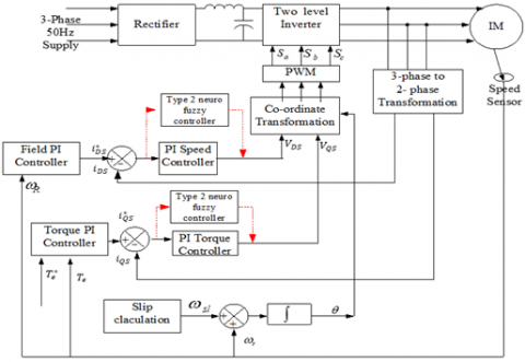
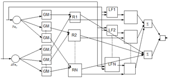
The suggested T2NFC-based IMD is presented in Figure 3. Figure 4 represents the T2NFC architectural design, which uses a seven-layer neural network architecture to combine neural network-based learning approaches with fuzzy logic. The T2NFC's inputs are the error in torque and changes of error in torque, with Te* serving as the command. The inputs are denoted by layer 1; the fuzzification is denoted by layer 2; the firing is denoted by layer 3; the consequence is denoted by layer 4; and the type reduction and defuzzification ways are achieved by the 5th, 6th, and 7th seventh layers, respectively. Fuzzy IF-THEN rules define a T2NFC, with type-2 fuzzy values as parameters in the antecedent and following parts of the rules. The suggested system's fuzzy ruleset is as follows:
if $e_{T}$ is $m_{1 j}$ and $\Delta e_{T}$ is $m_{2 j}$
Then, $y_{j}=\sum_{i=1}^{2} \omega_{i j} x_{i}+b_{j}$
where, $x_{1}=e_{T}, x_{2}=\Delta e_{T}$ are the input variables
$y_{j}$ is $m_{1 j} e_{T}+m_{2 j} \Delta e_{T}+b_{j}$
where, m1j and m2j are antecedent fuzzy sets, and wij and bj are training-estimated design parameters. The output MF is yj in this case.
1st Layer: This layer's nodes are all sharp input variables. This layer just receives input variables. This layer does not have any weights that may be changed.
Figure 3. Proposed type 2 neuro-fuzzy controller
Figure 4. Type 2 neuro-fuzzy system
2nd Layer: This layer contains of node MF, in which each input's crisp value is changed using a linguistic term, and in which an interval type-2 Gaussian MF is used. The interval can be represented as in equation by the higher and lower MF degrees with undetermined standard deviation (42).
$O_{j}^{2}=\bar{\mu}_{m 1 j}=e^{\left(-\frac{1}{2}\left(\frac{\left(x_{j}-c\right)^{2}}{\bar{\sigma}^{2}}\right)\right)} j=1,2$
$O_{j}^{2}=\bar{\mu}_{m 2 j}=e^{\left(-\frac{1}{2}\left(\frac{\left(x_{j}-c\right)^{2}}{\bar{\sigma}^{2}}\right)\right)} j=1,2$
$O_{j}^{2}=\bar{\mu}_{m 1 j}=e^{\left(-\frac{1}{2}\left(\frac{\left(x_{j}-c\right)^{2}}{\underline{\sigma}^{2}}\right)\right)} j=1,2$
$O_{j}^{2}=\bar{\mu}_{m 2 j}=e^{\left(-\frac{1}{2}\left(\frac{\left(x_{j}-c\right)^{2}}{\underline{\sigma^{2}}}\right)\right)} j=1,2$ (42)
where, c is the type-2 fuzzy sets' centre value. The parameters $\bar{\sigma}^{2}$ and ${\underline{\sigma}^{2}} 2$ are the upper-lower MF standard deviations. Here is the result for the node number, with superscript indicating the number of levels and Oj indicating the number of MF.
3rd layer: Every node in this layer uses the prod t-norm operator to determine the firing strength of a rule with the least mistake or variation in an error of two input weights, as shown in Eqns. (43) and (44) respectively.
$O_{j}^{3}=\overline{\omega_{l}}=\bar{\mu}_{m 1 j}\left(e_{T}\right) \bar{\mu}_{m 2 j}\left(\Delta e_{T}\right)$ (43)
$O_{j}^{3}=\underline{\omega}_{i}=\underline{\mu}_{m 1 j}\left(e_{T}\right) \underline{\mu}_{m 2 j}\left(\Delta e_{T}\right)$ (44)
where, $\bar{\omega}$ and $\underline{\omega}$ are the upper and lower outputs, respectively.
Every node in this layer determines its weight, which is normalized by firing strengths as shown in Eq. (45).
$\overline{\omega_{1}}=\frac{\overline{\omega_{1}}}{\sum_{i=1}^{M} \overline{\omega_{i}}}$ and, $\underline{\omega_{i}}=\frac{\underline{\omega_{i}}}{\sum_{i=1}^{M} \underline{\omega_{i}}}$ (45)
where, $\bar{\omega}_{i}$ and $\underline{\omega_{i}}$ are the normalised lower and higher outputs from the network's second hidden layer, respectively.
4th layer: The outputs of the linear functions in the subsequent portions for the two inputs as described in equation are in this layer (46).
$O_{j}^{4}=y_{j}=m_{1 j} e_{T}+m_{2 j} \Delta e_{T}+b_{j}$ (46)
5th Layer: As shown in equation, this layer calculates the product of the membership degrees $\underline{\omega_{i}}$ and $\bar{\omega}_{i}$ linear functions (47).
$O_{j}^{5}=y_{j}=q \sum_{i=1}^{M} y_{j} \underline{\omega_{i}}+(1-q) \sum_{i=1}^{M} y_{j} \overline{\omega_{l}}$ (47)
The weighting of each fired rule's lower and higher firing levels is determined by the design parameter q.
6th Layer: There are two summation blocks in this layer. The sum of the layer's output signals is computed by one of these blocks, while the total of layer 3's output signals is computed by the other.
7th Layer: Equations are used to calculate the output in this layer (48).
$u=\frac{q \sum_{i=1}^{M} y_{j} \underline{\omega_{i}}}{\sum_{i=1}^{M} \underline{\omega_{i}}}+\frac{(1-q) \sum_{i=1}^{M} y_{j} \overline{\omega_{i}}}{\sum_{i=1}^{M} \overline{\omega_{i}}}$ (48)
where, ‘u’ is the ultimate output and ‘M’ signifies the number of active rules. The constraint ‘q’ allows you to alter the lower or higher parts based on the system's level of assurance.
Training algorithm:
A backpropagation technique is used in the suggested T2NFC to automatically adjust the controller using least square estimation. The backpropagation procedure is exceptionally quick, with major characteristics such as location of a global lowest cost function, faster scaling, greater generalization, and decreased computation complexity. It uses a gradient descent mechanism to alter the weight. The cost function for training a T2NFC is shown in the diagram below.
$E=\frac{1}{2} \sum_{p=1}^{N}\left(u_{p}^{d}-u_{p}\right)^{2}$ (49)
where, $u_{p}^{d}$ pd is the predicted output for a pth particular section pattern, and up is the T2NFC's actual performance. For the proposed controller, N is the number of training instances. Equation describes the reduced objective function (50).
$E=\frac{1}{2}\left(T_{e}^{*}-T_{e}\right)^{2}=e^{2}$ (50)
Te* denotes the reference torque, whereas Te denotes the expected torque. To obtain the desired result, use Eq. (51) to determine the BP parameter rules for immediate parameter changes (53).
$\omega_{i j}(l+1)=\omega_{i j}(l)-\eta \frac{\partial E}{\partial \omega_{i j}}$ (51)
$b_{j}(l+1)=b_{j}(l)-\eta \frac{\partial E}{\partial b_{j}}$ (52)
$\sigma_{i j}(l+1)=\sigma_{i j}(l)-\eta \frac{\partial E}{\partial \sigma_{i j}}$ (53)
where, ‘η’ the learning rate, ‘l’ is the number of input neurons and ‘M’ is the number of rules, and is the learning rate (hidden neurons). The derivatives in (54)-(56) are calculated using the methods from Eqns. (51) to (53).
$\frac{\partial E}{\partial \omega_{i j}}=\frac{\partial E}{\partial u} \frac{\partial u}{\partial y_{j}} \frac{\partial y_{j}}{\partial \omega_{i j}}$$=\left(T_{e}-T_{e}^{*}\right) *\left(\frac{q \sum_{i=1}^{M} y_{j} \omega_{i}}{\sum_{i=1}^{M} \omega_{i}}+\frac{(1-q) \sum_{i=1}^{M} y_{j} \overline{\omega_{l}}}{\sum_{i=1}^{M} \overline{\omega_{l}}}\right) * x_{i}$ (54)
$\frac{\partial E}{\partial b_{j}}=\frac{\partial E}{\partial u} \frac{\partial u}{\partial y_{j}} \frac{\partial y_{j}}{\partial b_{i j}}=\left(T_{e}-T_{e}^{*}\right) *\left(\frac{q \sum_{i=1}^{M} y_{j} \underline{\omega_{i}}}{\sum_{i=1}^{M} \underline{\omega_{i}}}+\frac{(1-q) \sum_{i=1}^{M} y_{j} \overline{\omega_{i}}}{\sum_{i=1}^{M} \overline{\omega_{i}}}\right)$ (55)
$\frac{\partial E}{\partial \sigma_{i j}}=\sum \frac{\partial E}{\partial u}$$\left(\frac{\partial u}{\partial \underline{\omega_{i}}} \frac{\partial \underline{\omega_{i}}}{\partial \underline{\mu_{m i j}}} \frac{\partial \underline{\underline{\mu}}_{m i j}}{\partial \sigma_{i j}}+\frac{\partial u}{\partial \overline{\omega_{l}}} \frac{\partial \bar{\omega}_{l}}{\partial \overline{\mu_{m i j}}} \frac{\partial \bar{\mu}_{m i j}}{\partial \sigma_{i j}}\right)$ (56)
The T2NFC system's parameters may thus be changed by combining (51)-(53) and (54)-(55).
The parameter q, as previously discussed, allows us to change the lower or upper sections of the ending result. In this study, the value of q is optimised during learning from a starting value of 0.5 by applying Eq. (57) as follows:
$q(l+1)=q(l)-\eta \frac{\partial E}{\partial q}$ (57)
The following are the generic differential versions of the preceding equations:
$\frac{\partial E}{\partial u}=\left(T_{e}-T_{e}^{*}\right)$ (58)
$\frac{\partial u}{\partial \underline{\omega_{i}}}=q \frac{y_{j}-\underline{u}}{\sum_{i=1}^{M} \underline{\omega}_{i}}$ (59)
$\underline{u}=\frac{\sum_{i=1}^{M} y_{j} \underline{\omega_{i}}}{\sum_{i=1}^{M} \underline{\omega_{i}}}$ (60)
$\bar{u}=\frac{\sum_{i=1}^{M} y_{j} \overline{\omega_{l}}}{\sum_{i=1}^{M} \overline{\omega_{1}}}$ (61)
The gradient descent method's convergence is determined by the primary value of the learning rate. This value is commonly chosen from the [0, 1] range. A high learning rate can cause inconsistency in learning, whereas a low learning rate causes delayed learning. The learning rate must be carefully chosen for convergence.
The fuzzy rule set must be invoked first from the command window in order to start the simulations. The fuzzy file containing the rules written with the TS method is first opened in the MATLAB command window, and then the fuzzy editor (FIS) dialogue box appears. The .fis file is imported from the source file using the command window, and then opened using the file open command in the fuzzy editor dialogue box. The TS-fuzzy rules file is enabled once the .fis file is opened. The data is also exported to the workspace, and the simulations are run for a period of time (say 2 to 3 second). The rule view command can be used to view the written TS-fuzzy rules. The fuzzy editor tool box also has a visual rule viewer for the two inputs and one output. The simulations are run in MATLAB for 3 seconds with a set speed of 1450 rpm. It's worth noting that this TS-based fuzzy controller uses a file to invoke a set of fuzzy rules. The performance characteristics such as torque, speed, various currents, and so on are observed on the corresponding scopes when the simulation is run, as shown in Figures 5 to 7, accordingly.
A. Induction motor performance parameters during start-up
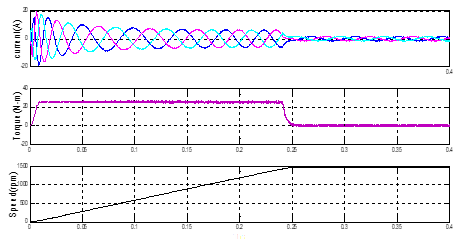
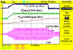
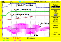
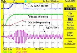
The performance of the drive at start up is depicted in Figure 5(a) - (c). For the induction motor drive the maximum current and the ripple content in the torque is reduced during starting in order to reach the early steady state. It is observed that there is a high current at the beginning. The high torque obtained with a PI controller is around 25 N-m, 26 N-m with T1NFC, and 27.5 N-m with T2NFC. With a PI controller, the motor drive achieves 1445 rpm in 0.265 seconds, 0.245 seconds with a T1NFC, and 0.23 seconds with a T2NFC With T2NFC, torque is greatly enhanced, and it is observed that the ripple content in the torque is reduced as compared to conventional method. Due to this, better speed response is attained.
(a) PI controllers
(b) Type 1 Neuro-Fuzzy controller
(c) Type 2 Neuro-Fuzzy controller
Figure 5. Induction motor performance characteristics during starting
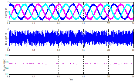
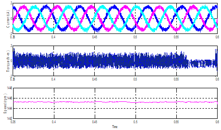
B. Steady State performance characteristics
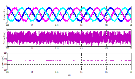
During the steady-state, the stator current, speed and, torque performance characteristics of the drive are shown in Figure 6 (a)-(c). The ripples in torque are determined to be between +1.4 and -1.4 when utilising the PI controller, between +1.2 and -1.2 with TINFC, and approximately +0.9 to -0.9 with T2NFC. The torque ripple with the proposed T2NFC is significantly reduced compared to the PI-controller thereby decreasing the magnitude and distortion of the motor current as evident from Figure 6 In fact, the oscillation in speed has almost disappeared with the proposed T2NFC-based drive as compared to the T1NFC which still has a tiny oscillation.
(a) With PI controllers
(b) Type 1 Neuro-Fuzzy controller
(c) Type 2 Neuro-Fuzzy controller
Figure 6. Steady state performance characteristics
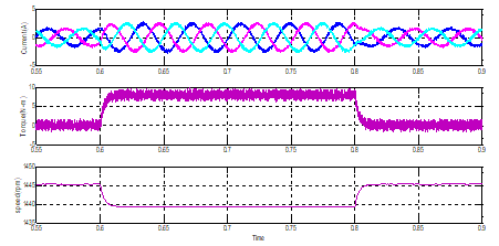
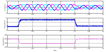
C. Response in load torque perturbation
The drive performances during the change in load torque are depicted in Figure 7 (a), (b), and (c). A load torque of 9 N-m is applied at 0.6 s to 0.8 s during the speed of 1445 rpm. During this, it is being observed that the steady state is reached earlier using the type 2 based controller compared to that of PI. And also enhanced performance parameters of the drive are obtained by step change in load torque. The torque ripple is minimized with T2NFC as compared to PI and T1NFC leading to less distortion of motor current.
(a) PI controller
(b) Type 1 Neuro-fuzzy controller
(c) Type 2 Neuro-fuzzy controller
Figure 7. Induction motor performance characteristics during load perturbation
To validate the performance of the traditional PI, T1NFC, and T2NFC based IM drives, a prototype model was built in the laboratory which is shown in Figure 8. By using dSPACE DS-2812 controller to develop the control algorithms as well as testing. The control technique is generated in Simulink tool, later with the help of MATLAB real-time workshop function the c-code is generated for real-time application. The appropriate gate pulses are created with the help of the master bit input-output, and Analog to Digital converters are utilised to line detected speed, currents, and voltage. Using the experimental setup and the dSPACE DS-2812, a PI, T1NFC, and T2NFC based IM drive is simulated and confirmed under various working situations, including beginning, steady-state, and different load conditions.
Figure 8. Experimental setup
The IMD beginning performance utilising PI, T1NFC, and T2NFC is represented in Figure 9 (a)-(c). With T2NFC, the rotor current, speed and torque are 3.96A, 1445 rpm, and 27.5 N-m, individually. The torque has been stabilised at 0.24s, which is a huge improvement. In comparison to PI and T1NFC’s, the speed response is much faster.
(a) PI controller
(b) Type 1 Neuro-fuzzy controller
(c) Type 2 Neuro-Fuzzy controller
Figure 9. Induction motor performance during starting
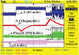
(a) PI Controller
(b) Type 1 Neuro-Fuzzy controller
(c) Type 2 Neuro-Fuzzy controller
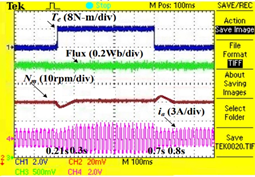
Figure 10. Steady state and dynamics in load of the T2NFC controlled drive
Figure 10 (a)-(c) shows the steady-state and dynamic performance of IM drives employing PI, T1NFC, and T2NFC. The suggested T2NFC significantly reduces torque ripples in this scenario; the ripple in torque is between -0.12 and +0.12, which is significantly smaller than T1NFC and PI controllers. As indicated in Figure 10, a load torque of 8 N-m is applied at 0.6s and withdrawn at 0.8s during the step shift in load torque. In comparison to T1NFC and PI controllers, the ripple in stator current and torque is greatly low with the suggested T2NFC, resulting in a smooth speed response.
The T2NFC-based IVC of IMD is developed in simulation and real-time prototype model with the help of dSPACE DS 2812 controller. Under various operating situations, the performance of IMD with PI, T1NFC, and T2NFC is compared. The PI-based IVC produces huge torque waves, which increases the time it takes for the IM to attain steady-state response in various operating zones. To increase the IM's dynamic response, the PI controller is swapped with T1NFC. The motor's performance isn't much increased due to T1NFC's constraints. T1NFC is also replaced with T2NFC for a quicker dynamic response. When related to the PI and T1NFC controllers, high starting current is minimizes and the torque rises up to 4% through the beginning stage with T2NFCs. As a result, the speed reaches rapidly. When compared to the T1NFC controller, the current ripple is minimised during the steady-state condition because the torque ripple is decreased by 33% and speed fluctuations are decreased. When related to traditional PI and T1NFC controllers, the total ripple content is decreased during step change load torque. T2NFC torque controllers outperform then PI and T1NFC torque controllers in terms of drive performance in various working circumstances.
The suggested technique employs type-2 Gaussian MFs with undetermined standard deviation. Upcoming study might include extending the suggested technique to different kind of MFs, such as Gaussian type-2 MFs with unknown centres, Elliptic type-2 MFs, and so on.
|
IM drive parameters |
|
|
Power |
= 3.7kW |
|
Voltage |
= 415V |
|
Speed |
= 1445 rpm |
|
Frequency |
= 50Hz |
|
Pole pairs |
= 2 |
|
Resistance of the stator |
= 7.34Ω |
|
Leakage inductance of the stator |
= 0.021H |
|
Resistance of the rotor |
= 5.64 Ω |
|
Leakage inductance of the rotor |
= 0.021H |
|
Mutual Inductance |
= 0.5H |
|
Friction coefficient |
= 0.035kg-m2/s |
|
Inertia coefficient |
= 0.16kg-m2 |
|
PI-speed control |
= 20/0.02 |
|
PI-torque control |
= 10/0.01 |
|
Tuning rate of the weight |
= 0.05 |
|
Tuning rate of the MFs |
= 0.005 |
[1] Harnefors, L. (2001). Design and analysis of general rotor-flux-oriented vector control systems. IEEE Transactions on Industrial Electronics, 48(2): 383-390. https://doi.org/10.1109/41.915417
[2] Khambadkone, A.M., Holtz, J. (1991). Vector-controlled induction motor drive with a self-commissioning scheme. IEEE Transactions on Industrial Electronics, 38(5): 322-327. https://doi.org/10.1109/41.97551
[3] Vas, P. (1998). Sensor Less Vector and Direct Torque Control. London, U.K.: Oxford Univ. Press, Jan. 1998, 400-535.
[4] Dominic, D.A., Chelliah, T.R. (2014). Analysis of field-oriented controlled induction motor drives under sensor faults and an overview of sensorless schemes. ISA Transactions, 53(5): 1680-1694. https://doi.org/10.1016/j.isatra.2014.04.008
[5] Telford, D., Dunnigan, M.W., Williams, B.W. (2001). A novel torque-ripple reduction strategy for direct torque control of induction motor. IEEE Transactions on Industrial Electronics, 48(4): 867-870. https://doi.org/10.1109/41.937422
[6] Umanand, L., Bhat, S.R. (1995). Online estimation of stator resistance of an induction motor for speed control applications. IEE Proceedings-Electric Power Applications, 142(2): 97-103. https://doi.org/10.1049/ip-epa:19951568
[7] Kumar, N., Chelliah, T.R., Srivastava, S.P. (2015). Adaptive control schemes for improving dynamic performance of efficiency-optimized induction motor drives. ISA Transactions, 57: 301-310. https://doi.org/10.1016/j.isatra.2015.02.011
[8] Briz, F., Degner, M.W., Lorenz, R.D. (2000). Analysis and design of current regulators using complex vectors. IEEE Transactions on Industry Applications, 36(3): 817-825. https://doi.org/10.1109/28.845057
[9] Jung, J., Lim, S., Nam, K. (1997). PI type decoupling control scheme for high speed operation of induction motors. In PESC97. Record 28th Annual IEEE Power Electronics Specialists Conference. Formerly Power Conditioning Specialists Conference 1970-71. Power Processing and Electronic Specialists Conference 1972, 2: 1082-1085. https://doi.org/10.1109/PESC.1997.616877
[10] Harnefors, L., Nee, H.P. (1998). Model-based current control of AC machines using the internal model control method. IEEE Transactions on Industry Applications, 34(1): 133-141. https://doi.org/10.1109/28.658735
[11] Bahrani, B., Kenzelmann, S., Rufer, A. (2010). Multivariable-PI-based $ dq $ current control of voltage source converters with superior axis decoupling capability. IEEE Transactions on Industrial Electronics, 58(7): 3016-3026. https://doi.org/10.1109/TIE.2010.2070776
[12] Jain, J.K., Ghosh, S., Maity, S., Dworak, P. (2017). PI controller design for indirect vector controlled induction motor: A decoupling approach. ISA Transactions, 70: 378-388. https://doi.org/10.1016/j.isatra.2017.05.016
[13] Krishnan, R. (2001). Electric Motor Drives: Modeling, Analysis, and Control. Pearson.
[14] Arulmozhiyal, R., Baskaran, K., Manikandan, R. (2011). A fuzzy based PI speed controller for indirect vector controlled induction motor drive. In India International Conference on Power Electronics 2010 (IICPE2010), pp. 1-7. https://doi.org/10.1109/IICPE.2011.5728102
[15] Hannan, M.A., Abd Ali, J., Hussain, A., Hasim, F.H., Amirulddin, U.A.U., Uddin, M.N., Blaabjerg, F. (2017). A quantum lightning search algorithm-based fuzzy speed controller for induction motor drive. IEEE Access, 6: 1214-1223. https://doi.org/10.1109/ACCESS.2017.2778081
[16] Rafa, S., Larabi, A., Barazane, L., Manceur, M., Essounbouli, N., Hamzaoui, A. (2014). Implementation of a new fuzzy vector control of induction motor. ISA Transactions, 53(3): 744-754. https://doi.org/10.1016/j.isatra.2014.02.005
[17] Lokriti, A., Salhi, I., Doubabi, S., Zidani, Y. (2013). Induction motor speed drive improvement using fuzzy IP-self-tuning controller. A real time implementation. ISA Transactions, 52(3): 406-417. https://doi.org/10.1016/j.isatra.2012.11.002
[18] Ramesh, T., Panda, A.K., Kumar, S.S. (2013). Type-1 and type-2 fuzzy logic speed controller based high performance direct torque and flux controlled induction motor drive. In 2013 Annual IEEE India Conference (INDICON), pp. 1-6. https://doi.org/10.1109/INDCON.2013.6725947
[19] Ramesh, T., Panda, A.K., Kumar, S.S. (2015). Type-2 fuzzy logic control based MRAS speed estimator for speed sensorless direct torque and flux control of an induction motor drive. ISA Transactions, 57: 262-275. https://doi.org/10.1016/j.isatra.2015.03.017
[20] Giribabu, D., Vardhan, R.H., Prasad, R.R. (2016). Multi level inverter fed indirect vector control of induction motor using type 2 fuzzy logic controller. In 2016 International Conference on Electrical, Electronics, and Optimization Techniques (ICEEOT), pp. 2605-2610. https://doi.org/10.1109/ICEEOT.2016.7755164
[21] Durgasukumar, G., Abhiram, T., Pathak, M.K. (2012). TYPE-2 fuzzy based SVM for two-level inverter fed induction motor drive. In 2012 IEEE 5th India International Conference on Power Electronics (IICPE), pp. 1-6. https://doi.org/10.1109/IICPE.2012.6450468
[22] Naik, N.V., Singh, S.P. (2015). A comparative analytical performance of F2DTC and PIDTC of induction motor using DSPACE-1104. IEEE Transactions on Industrial Electronics, 62(12): 7350-7359. https://doi.org/10.1109/TIE.2015.2463758
[23] Naik, N.V., Panda, A., Singh, S.P. (2015). A three-level fuzzy-2 DTC of induction motor drive using SVPWM. IEEE Transactions on Industrial Electronics, 63(3): 1467-1479. https://doi.org/10.1109/TIE.2015.2504551
[24] Durgasukumar, G., Pathak, M.K. (2012). Comparison of adaptive neuro-fuzzy-based space-vector modulation for two-level inverter. International Journal of Electrical Power & Energy Systems, 38(1): 9-19. https://doi.org/10.1016/j.ijepes.2011.10.017
[25] Sukumar, D., Jithendranath, J., Saranu, S. (2014). Three-level inverter-fed induction motor drive performance improvement with neuro-fuzzy space vector modulation. Electric Power Components and Systems, 42(15): 1633-1646. https://doi.org/10.1080/15325008.2014.927022
[26] Durgasukumar, G., Pathak, M.K. (2012). Comparison of adaptive Neuro-Fuzzy-based space-vector modulation for two-level inverter. International Journal of Electrical Power & Energy Systems, 38(1): 9-19. https://doi.org/10.1016/j.ijepes.2011.10.017
[27] Sathishkumar, H., Parthasarathy, S.S. (2017). A novel fuzzy logic controller for vector controlled induction motor drive. Energy Procedia, 138: 686-691. https://doi.org/10.1016/j.egypro.2017.10.201
[28] Pakkiraiah, B., Sukumar, G.D. (2017). Enhanced performance of an asynchronous motor drive with a new modified adaptive Neuro-Fuzzy inference System-Based MPPT controller in interfacing with dSPACE DS-1104. International Journal of Fuzzy Systems, 19(6): 1950-1965. https://doi.org/10.1007/s40815-016-0287-5
[29] Masumpoor, S., Khanesar, M.A. (2015). Adaptive sliding-mode type-2 neuro-fuzzy control of an induction motor. Expert Systems with Applications, 42(19): 6635-6647. https://doi.org/10.1016/j.eswa.2015.04.046
[30] Abiyev, R.H., Kaynak, O., Alshanableh, T., Mamedov, F. (2011). A type-2 neuro-fuzzy system based on clustering and gradient techniques applied to system identification and channel equalization. Applied Soft Computing, 11(1): 1396-1406. https://doi.org/10.1016/j.asoc.2010.04.011