Amine Zeggai* | Farid Benhamida | Riyadh Bouddou
© 2021 IIETA. This article is published by IIETA and is licensed under the CC BY 4.0 license (http://creativecommons.org/licenses/by/4.0/).
OPEN ACCESS
The cost of electricity for the reverse osmosis desalination process is up to 50% of the cost per cubic meter of water produce. Currently, the reduction of energy consumption is the main objective of the research on reverse osmosis plants. This document presents a power system analysis of the seawater desalination plant in Algeria with different load scenarios with a power of 50 MW made available by the electricity company Sonelgaz and a distribution level of 220/11/0.69/0.4 kV and a 2 MW diesel generator at the 0.4 kV level. The objective of this study is to analyze and dimension a general distribution network of an industrial customer through the power flow with different load and contingency scenarios (full load, full load N-1, low load, emergency system) to know and control its optimal and flexible operation. In a second step, the dimensioning of different protective devices is planned through a short circuit analysis of this network in order to evaluate the performance of the system. The ETAP program is used to carry out our simulation of this industrial plant and the effectiveness of the results is proven by comparisons with real measurements for the power flow analysis on the one hand and on the other hand with the results obtained by the builder for the short circuit analysis.
load flow analysis, real industrial plant, short circuit analysis, different load scenario, ETAP (electrical transient analyzer program)
Almost 40% of the world's population lacks freshwater, while more than 95 percent of the water on earth is saline and cannot be used as drinking water or for irrigation purposes [1, 2]. Desalination appears as a solution to obtain additional drinking water or process water for people, industry, and agriculture. But even if it is developing, the technique has its limits in terms of cost and energy consumption. The power system deployed must be capable of meeting the load requirement under defined contingencies. To monitor, to maintain stability under various operating conditions, and to manage these complex industrial power systems, different additional sophisticated simulation software’s are used. To facilitate the supply of reliable power, the operation team needs to create different scenarios for power flow, short circuit, and stability studies in advance to check the constraints in the system, if any. Proactive actions can be taken based on these simulation study results to [3-5].
• Improves practical tension profiles.
• Minimize active and reactive losses.
• Optimize circuit usage.
• Minimize disruption to process plant operations.
• Check the dimensioning and setting of protective devices.
• Identify transformer tap settings [6].
Continuous and comprehensive analysis of an electrical system is required to assess the current state of the system and to evaluate the optional plans for system expansion. Due to the electrical power system of the whole plant involving the requirements of power source, distribution network, manufacturing, and technical management, it is higher than power supply companies in medium-sized industries under controlled conditions [7-11]. The power system model of an industrial complex is presented here power flow analysis (1) simulation using ETAP software version 16.0.0.
The acceptable voltage limits are as per the standard IS-12360- 2006. The power flow simulations are carried out for identifying the best-operating conditions provided under the guidelines of process requirements, and (2) simulation of short circuit analysis to check the rating of electrical devices under fault conditions and to establish the electrical distribution system at various voltage levels [12-15].
2.1 Teste system
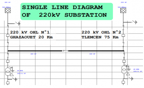
The plant electrical system is receiving a power supply from Sonelgaz at 220 kV. Each feeder will have a 45 MW capacity for the full plant operation. The 220 kV system design configuration is an “H” design (Figure 1).
The supply voltage is step-down to 11 kV via 65 MVA transformers, where it is fed to the main switch room. The main switch room distribute the power to the respective area within the plant. The voltage level at the sub-station is further step down from 11 kV to 0.4 kV for motors, VFDs, and 11 kV to 0.69 kV for the VFD driven pumps like Seawater Intake Pump, RO feed pumps. 11 kV system is earthed through the earthing transformer to limit the earth fault current to the max of 1000 A. For 400 V, 3-phase 4 wires with the neutral point solidly connected to the earthing circuit. Two separate line feeders from Ghazaouet and Tlemcen feeding the 220 kV substation located at the south of the plant. Each line will be feeding the power transformers which will step down the voltage to 11 kV and feed the 11 kV main switchgear located in the main switchgear room adjacent to the 220 kV substation.
To have the flexibility of the feeding power transformers from any of the lines, the interconnection of the lines was done with 220 kV isolator, Q13 as indicated in the 220 kV Single line diagram. Line feeders from the Sonelgaz are provided with the main and back up distance protection systems. Each power transformer is rated for the full load capacity of the plant giving the 100% redundant power supply to the 11 kV mainboard. This 11 kV main board is provided with the bus section breaker to have the redundancy.
The complete electrical system of the plant is designed with redundancy so that the failure of any of the transformer/feeders will not affect the operating capacity of the plant.
Figure 1. Single line diagram of 220 kV substation, “H” design
The operation of the network is such that the 2 lines feed each section of the busbar, one on the left and the other on the right. Thus, both input circuit breakers are in the "on" position and the circuit breaker in the closed position. The circuit breaker of the busbar coupling is in the "service" position and the circuit breaker in the open position. Both earthing switches must be in the "OFF" position. The station is fully charged.
The desalination station is divided into 6 zones which supply the 220/11 kV "zone 1 or 70" 220/11 kV substation located south of the plant via two separate 220 kV high voltage lines from the Ghazaouet 20 km high voltage substation and the Tlemcen 75 km high voltage substation, which supply the 220/11 kV substation located south of the plant, which ensures the power supply for the entire plant during normal operation:
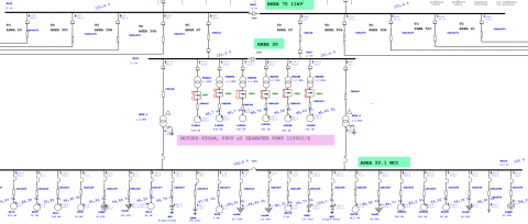
Area 70 or 1 (Figure 2): Supplied by two 220 kV lines, each line feeds a 65 MVA power transformer which lowers the voltage to 11 kV which ensures the power supply of the 11 kV main busbar.
Area 20 or 2 (Figure 2): Supplied by two 11 kV cables, each with a 300 mm2, single-pole 1 per phase or incoming feeds an 11 kV busbar (outgoing feeder which arrives via the left main 11 kV busbar feeds the left main 11 kV busbar of area 2 and incoming feeder which arrives via the right main 11 kV busbar feeds the right main 11 kV busbar of area 2, the same network architecture for all the following areas ) and the two busbars 400 V right and left, each supplied by a 1.6 MVA 11/0.4 kV transformer which supplies from a right busbar 11kV outgoing feeder for the right 400 V busbar "20. 1MCC" and another 11 kV right-hand busbar outgoing feeder for the 400V right-hand busbar outgoing feeder with two circuit breakers of the coupling in open position between the two busbars of the same voltage 11 kV and 400 V.
Area 40 or 6 (Figure 2): Supply by two 11 kV cables, each with a 300 mm2, single-pole 2 per phase or incoming feeds one busbar and the two 11 kV busbar sets and the two 400 V busbar sets "40. 1MCC " right and left supply each one by a 740 kVA 11/0,4 kV transformer which supplies by one 11 kV right busbar outgoing feeder for the 400 V right busbar and another 11 kV right busbar outgoing feeder for the 400 V right busbar with two circuit breakers of the coupling in open position between the two busbars of the same voltage 11 kV and 400 V.
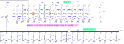
Area 30A or 3 (Figure 3): Supply by two 11 kV cables, each with a 300 mm2, single-pole 2 per phase or incoming feeds one busbar and the two 11 kV busbar sets and the two 400 V busbar sets "30. 2MCC " right and left supply each one by a transformer of 2 MVA 11/0,4 kV which supplies by one outgoing feeder of right busbar 11 kV for the 400 V right busbar and another outgoing feeder of right busbar 11 kV for the 400 V right busbar with two circuit breakers of the coupling in open position between the two busbars of the same voltage 11 kV and 400 V.
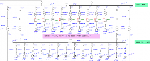
Area 30B or 4 (Figure 3): Supply by two 11 kV cables, each with a 300 mm2, single-pole 2 per phase or incoming feeds one busbar and both 11 kV busbars with one circuit breaker of the coupling in the open position. And the 400V busbar sets:
The two sets of 400 V "30.1MCC" right and left 400 V busbars, each supplied by a 1.6 MVA 11/0.4 kV transformer which supplies one 11 kV right busbar outlet for the 400 V right busbar and another 11 kV right busbar outlet for the 400 V right busbar with a circuit breaker in the open position.
The two sets of 400 V "30.3MCC" right and left busbars are each supplied by a 2.5 MVA 11/0.4 kV transformer which supplies one 11 kV right-hand busbar feeder for the 400 V right-hand busbar and another 11 kV right-hand busbar feeder for the 400 V right-hand busbar with a circuit breaker in the open position.
Area 30C or 5 (Figure 3): Supply by two 11 kV cables, each with a 300 mm2, single pole 2 per phase or incoming feeds one busbar and both 11 kV busbar sets and both 400 V busbar sets "30. 4MCC " right and left supply each one by a transformer of 2,5 MVA 11/0,4 kV which supplies by one outgoing feeder of right busbar 11 kV for the 400 V right busbar and another outgoing feeder of right busbar 11 kV for the 400 V right busbar with two circuit breakers of the coupling in open position between the two busbar sets of the same voltage 11 kV and 400 V.
Electrical system network data is modeled in the software for system analysis. Important inputs to an effective system study are:
Identification of all loads specifically split of motive and non-motive loads.
_Power Grid, connection (3 phase), operation mode (swing, voltage control, Mvar control, PF control), voltage, grounding, and power of a short circuit.
_Bus, status (normal or priority), nominal kV (magnitude and angle), load diversity factors (max and min), voltage limit (max and min), and feeder tag.
_Transformer, their rated characteristic, power, voltages (primary and secondary), cooling mode, impedance, a ratio of tap-changer, connection and grounding method, and short-circuit voltage U%.
_Generators, including MVA, voltage control, operation mode, power factory, efficiency, number of pole, impedances, dynamic model, grounding, and inertia.
_Circuit Breaker (Low/High voltage), ID, condition, status, rated kV/Amp, making peak, breaking time, time constant, thermal current Ith, min delay and break time.
_Transmission line/ Cable, length (km), physical, conductor type/section, unit system, frequency, impedance, temperature, and configuration type.
_Measuring devices, ammeter, voltmeter, potential/current transformer.
_Future provisions to be added according to different scenarios.
2.2 Assumptions & operating conditions for power flow study
Following are the assumptions and network operating conditions for the simulation and analysis carried out. Load flow calculations are based on the Adaptive Newton Raphson method.
Full Load (Scenario 1): the factory operates normally all the areas in service and all its consumption through networks Sonelgaz two lines 220 kV with the full capacity of production treated water 200 MLD.
Full Load N-1(Scenario 2): like scenario 1 with a loss of a 220 kV line, all electrical busbar high voltage 11kV and low voltage 400 V of MCC supplied by right circuit breakers provided that the circuit breakers of the coupling is closed after opening the left circuit breakers (all plant supplied with the power transformer 65 MVA number 2 and all right transformer of each area).
Low Load (Scenario 3): the plant is on standby for maintenance or rehabilitation, for example, 90% of the loads is stopped except the lighting, the catch, ... ex and all its consumption through the networks Sonelgaz lines 220 kV with low capacity of production treated water 20 MLD.
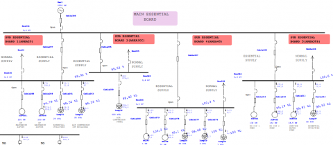
Emergency System (Scenario 4): In this case (a total missing of the Sonelgaz power supply), the diesel group with 2000 kVA supplies all emergency loads of main essential board, just to protect property and people with the total loss of treated water production.
Tap Chargers (220/11 kV transformer) is a device for adding or removing turns to the main winding of the Power Transformer that can thus be adapted to the load conditions on the network to maintain the voltage at an optimal level at the 11 kV bus bar.
2.3 Short circuit study
A Short-circuit study is very important for the dimensioning of safety devices such as circuit breakers. The knowledge of the value of the short-circuit Isc has all the places of the installation of a company with deferent scenarios of the load and the type of the short-circuit (defect three-phase, defect biphasic to the ground or insulated, defect single-phase) allows or one wants to place a protection device and that the breaking capacity of the circuit breaker and much higher than the current of the fault at this place, all the study and the simulation based on the norm 60909, it applies to all basic and high voltage ac systems.
3.1 Simulation of load flow analysis
Load flow models must be validated before making any recommended system modifications. The validation of our system is carried out by acquiring the actual values of the electrical variables and comparing the simulation results with the actual measurements of the system using the operating experience with different modes of operation.
The power flow comparison between the actual measurement result and calculation result by ETAP is given in Table 1. It should be noted that the ETAP results are the same as the measured result with a lack of precision of the electrical measuring instrument. ETAP software allows very accurate and practical analysis with less required memory.
Once the electrical model of the desalination plant was completed, Power Flow was executed. It should be understood that the convergence of power flows is the simplest way to check whether the given power system is feasible and whether the input data is consistent. During the Power Flow of the different areas (70, 20, 30A, 30B, 30C, 40) of the plant with different load scenarios and emergency conditions (full load, full load N-1, low load, emergency system), we verify that:
- The input data for the system is consistent and that the system is feasible.
- The bus voltages are within +/- 5%.
- String loads are within limits, less than 80% of loads.
- The load on power transformers is within limits, less than 80% load.
- The dimensions of the feeders are correct.
Scenario 1 (Figure 2 & Figure 3): During the power flow, the total power consumed is 50.525 MW, 22.608 MVar with a power factor is 91.3% (see Table 2);
The bus voltages are less than +/- 5% with a slight voltage drop for the buses351 94.9% that feeds motor 315 kW of ERS Booster, bus38 and bus40 95% that feeds motors 200 kW of UF Backwash it is three motors control it with Variable Frequency Drive VFD 200 kW and according to the needs of the process, it is very rare to reach the maximum power so the conclusion the bus voltages are within limits.
An overload of the cable 348 that feeds RO cleaning heater after a research in the maintenance history report of the plant we were found that a problem of the very short life of the heater elements so the conclusion is that there is a wrong dimensioning in this part.
For the power factor 91.3% according to the Algerian standards for high voltage type B customers, a reagent consumption not exceeding 50% (PF equal 89.44%) of that of the active energy. The reagent consumed above this level is invoiced to the customer in the form of a malus and below this level, the customer is given a bonus. In conclusion, the power factor is good with a reagent consumption of 44.75%, and the invoice is improved [16, 17].
Scenario 2: During the power flow, the total power consumed is 49.952 MW, 25.73 MVar with a power factor is 88.9 (see Table 3);
For the bus128, 351…355 that feeds ERS Booster motor 315kW of bus voltage% Bethwin 93.5 and 94.4 the bus38 93.9% and bus40 93, 1% that feeds Backwash motor 200 kW, it is all motors control it with VFD 200 kW and according to the needs of the process, it is very rare to reach the maximum power so the conclusion the bus voltages are within limits.
For the bus 37&39 93.9% that feeds Neutralisation motor 22.5 kW after a research in the maintenance history report of the plant we were found that a problem of the very short life (low wedding).
An overload of the Transformer TX20.1 (11/0.4 kV 1.6 MVA) 108.5% that feeds MCC 20.1 (Motor Control Center), after a study of the production process of this part we have concluded that this scenario of all these loads running at full capacity and at the same time is a low probability, but it is not impossible, so despite this it is necessary to consider this probability.
Figure 2. Load flow analysis of area 70, 20, 40 & main essential board with full load scenario
Figure 3. Load flow analysis of area 30A, 30B & 30C with full load scenario
Table 1. Comparison of the results of the load flow simulation on ETAP and the actual measurement in the installation with different load scenarios
|
Calculation ETAP % Bus Voltage |
Actual Measurement % Bus Voltage |
|||||||||
|
Area |
Voltage |
Name bus |
Scenario 1 |
Scenario 2 |
Scenario 3 |
Scenario 4 |
Scenario 1 |
Scenario 2 |
Scenario 3 |
Scenario 4 |
|
1 or 70 |
230 kV |
bus 1 |
100 |
100 |
100 |
/ |
100 |
100 |
100 |
/ |
|
bus 2 |
100 |
100 |
100 |
/ |
100 |
100 |
100 |
/ |
||
|
11 kV |
bus 3 |
101.6 |
101.3 |
101.7 |
/ |
101 |
101 |
102 |
/ |
|
|
bus 4 |
101.4 |
101.3 |
101.7 |
/ |
101 |
101 |
102 |
/ |
||
|
2 or 20 |
11 kV |
bus 7 |
101.4 |
101.2 |
101.7 |
/ |
101 |
101 |
102 |
/ |
|
bus 8 |
101.5 |
101.2 |
101.7 |
/ |
101 |
101 |
102 |
/ |
||
|
400V |
bus 13 |
100.6 |
98.79 |
101.2 |
/ |
100 |
99 |
101 |
/ |
|
|
bus 14 |
100 |
98.79 |
101.1 |
/ |
100 |
99 |
101 |
/ |
||
|
bus 336 |
99.92 |
99.63 |
101.1 |
99.79 |
99 |
100 |
101 |
99.8 |
||
|
3 or 30A |
11 kV |
bus 104 |
101.6 |
101.2 |
101.7 |
/ |
101 |
101 |
102 |
/ |
|
bus 105 |
101.4 |
101.2 |
101.7 |
/ |
101 |
101 |
102 |
/ |
||
|
400V |
bus 116 |
100.8 |
99.62 |
102.3 |
/ |
100 |
100 |
102 |
/ |
|
|
bus 117 |
100.7 |
99.62 |
102.2 |
/ |
100 |
100 |
102 |
/ |
||
|
4 or 30B |
11 kV |
bus 155 |
101.6 |
101.2 |
101.7 |
/ |
101 |
101 |
102 |
/ |
|
bus 156 |
101.4 |
101.2 |
101.7 |
/ |
101 |
101 |
102 |
/ |
||
|
400V |
bus 184 |
100.6 |
99.54 |
102.2 |
/ |
100 |
100 |
102 |
/ |
|
|
bus 185 |
100.8 |
99.54 |
102.5 |
/ |
100 |
100 |
102 |
/ |
||
|
bus 201 |
100.9 |
99.83 |
102.1 |
/ |
101 |
101 |
102 |
/ |
||
|
bus 202 |
100.8 |
99.83 |
102.1 |
/ |
101 |
101 |
102 |
/ |
||
|
bus 346 |
100.6 |
99.62 |
102 |
100 |
100 |
100 |
101 |
100 |
||
|
5 or 30C |
11 kV |
bus 220 |
101.4 |
101.2 |
101.7 |
/ |
101 |
101 |
102 |
/ |
|
bus 221 |
101.6 |
101.2 |
101.7 |
/ |
101 |
101 |
102 |
/ |
||
|
400V |
bus 233 |
101 |
99.56 |
102.5 |
/ |
101 |
100 |
102 |
/ |
|
|
bus 234 |
100.4 |
99.56 |
101.7 |
/ |
100 |
100 |
102 |
/ |
||
|
bus 342 |
99.53 |
98.71 |
102.1 |
100.5 |
99.4 |
99 |
102 |
100.6 |
||
|
4 or 40 |
11 kV |
bus 265 |
101.6 |
101.2 |
101.7 |
/ |
101 |
101 |
102 |
/ |
|
bus 266 |
101.4 |
101.2 |
101.7 |
/ |
101 |
101 |
102 |
/ |
||
|
400V |
bus 298 |
100.3 |
98.97 |
101.1 |
/ |
100 |
100 |
101 |
/ |
|
|
bus 300 |
100.5 |
98.97 |
101.5 |
/ |
101 |
99 |
102 |
/ |
||
|
bus 304 |
100.3 |
98.97 |
101.1 |
99.35 |
100.3 |
99 |
101 |
99.4 |
||
Table 2. Load flow report of “Bus 3 & 2” and Critical report of power flow with scenarios 1(full load)
|
Load Flow Report |
||||||||||||||||||
|
Voltage |
Generation |
Load |
Load Flow |
|||||||||||||||
|
kV |
% Mag |
Ang |
MW |
Mvar |
MW |
Mvar |
ID |
MW |
Mvar |
Amp |
%FP |
|||||||
|
220.000 |
100.000 |
0.0 |
50.525 |
22.608 |
0 |
0 |
Bus3 |
24.318 |
10.899 |
69.9 |
91.3 |
|||||||
|
Bus2 |
26.209 |
11.709 |
75.3 |
91.3 |
||||||||||||||
|
Critical Report |
||||||||||||||||||
|
Device ID |
Type |
Condition |
Rating/Limit |
Unit |
Operating |
% Operating |
Phase type |
|||||||||||
|
Bus 351 |
Bus |
Under Voltage |
0.415 |
kV |
0.394 |
94.9 |
3-Phase |
|||||||||||
|
Cable 348 |
Cable |
Overload |
465.6 |
Amp |
508.41 |
109.2 |
3-Phase |
|||||||||||
Table 3. Load flow report of “Bus 3 & 2” and Critical report of power flow with scenarios 2 (full load N-1)
|
Load Flow Report |
||||||||||||||||||
|
Voltage |
Generation |
Load |
Load Flow |
|||||||||||||||
|
kV |
% Mag |
Ang |
MW |
Mvar |
MW |
Mvar |
ID |
MW |
Mvar |
Amp |
% FP |
|||||||
|
220.000 |
100.000 |
0.0 |
49.952 |
25.730 |
0 |
0 |
Bus 3 |
49.952 |
25.730 |
147.5 |
88.9 |
|||||||
|
Bus 2 |
0.000 |
0.000 |
0.0 |
0.0 |
||||||||||||||
|
Critical Report |
||||||||||||||||||
|
Device ID |
Type |
Condition |
Rating/Limit |
Unit |
Operating |
% Operating |
Phase type |
|||||||||||
|
Bus 128 |
Bus |
Under Voltage |
0.415 |
kV |
0.391 |
94.2 |
3-Phase |
|||||||||||
|
Bus 134 |
Bus |
Under Voltage |
0.415 |
kV |
0.39 |
94.4 |
3-Phase |
|||||||||||
|
Bus 31 |
Bus |
Under Voltage |
0.415 |
kV |
0.39 |
94.5 |
3-Phase |
|||||||||||
|
Bus 351 |
Bus |
Under Voltage |
0.415 |
kV |
0.39 |
94.1 |
3-Phase |
|||||||||||
|
Bus 352 |
Bus |
Under Voltage |
0.415 |
kV |
0.39 |
94.4 |
3-Phase |
|||||||||||
|
Bus 353 |
Bus |
Under Voltage |
0.415 |
kV |
0.39 |
94.4 |
3-Phase |
|||||||||||
|
Bus 354 |
Bus |
Under Voltage |
0.415 |
kV |
0.39 |
94.4 |
3-Phase |
|||||||||||
|
Bus 354 |
Bus |
Under Voltage |
0.415 |
kV |
0.39 |
94.4 |
3-Phase |
|||||||||||
|
Bus 37 |
Bus |
Under Voltage |
0.415 |
kV |
0.39 |
94.9 |
3-Phase |
|||||||||||
|
Bus 38 |
Bus |
Under Voltage |
0.415 |
kV |
0.39 |
94.1 |
3-Phase |
|||||||||||
|
Bus 39 |
Bus |
Under Voltage |
0.415 |
kV |
0.39 |
94.9 |
3-Phase |
|||||||||||
|
Bus 40 |
Bus |
Under Voltage |
0.415 |
kV |
0.39 |
94.1 |
3-Phase |
|||||||||||
|
Cable 348 |
Cable |
Overload |
465.6 |
Amp |
508.41 |
110.3 |
3-Phase |
|||||||||||
|
TX20.1 |
Transformer |
Overload |
1.6 |
MVA |
508.41 |
108.5 |
3-Phase |
|||||||||||
Table 4. Load flow report of “Bus 3 & 2” of power flow with scenarios 3 (low load)
|
Load Flow Report |
|||||||||||
|
Voltage |
Generation |
Load |
Load Flow |
||||||||
|
kV |
% Mag |
Ang |
MW |
Mvar |
MW |
Mvar |
ID |
MW |
Mvar |
Amp |
%FP |
|
220.000 |
100.000 |
0.0 |
4.730 |
1.315 |
0 |
0 |
Bus 3 |
4.270 |
1.054 |
11.5 |
97.1 |
|
Bus 2 |
0.460 |
0.261 |
1.4 |
86.9 |
|||||||
Figure 4. Load flow analysis of area 20.1MCC with scenario 2a
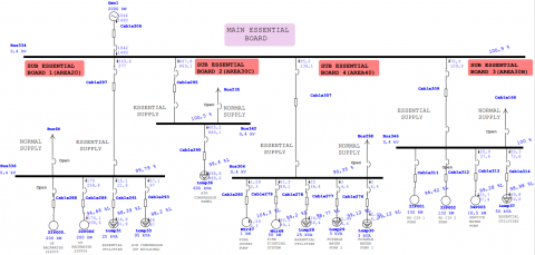
Figure 5. Load flow analysis of the main essential board with an emergency scenario
Therefore, we have deepened our study for this case and proposed three other scenarios of MCC 20.1 (low voltage of area 20) in scenario 2 below;
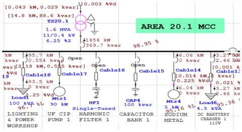
Scenario 2a: The same of scenario 2 with stopped the UF CIP motors 1&2 90 kW each one and Neutralization motor 3 18.5 kW according to the advice and the need for operation (see Figure 4).
Here are the results of the load flow from this scenario: 1458 kW, 177.2 kVar, 2126 A, 99% PF with a voltage in the busbar 14 is 99.73%.
It has a little overload on the 91.7% transformer, but it can support this load and works correctly until the time of maintaining the second electrical supply and ensure production.
Scenario 2b; The same as scenario a with the lack of Capacity bank1 100 kVar and Harmonic filter1 105 kVar (see Figure 6).
The color of the transformer changes (pink) in the simulation of the load flow, It is an alarm that means that the transformer is on overload and must react as quickly as possible to avoid damage to the transformer and stopped the production because the transformer is very costly, due to the increase of the current from 2126A to 2189A (63A) with a 100% increase of the reactive power (kVar) from 177.2 to 369.7 and consequently a decrease of the power factor by 2.3% (99.2% to 96.9%) and of the busbar voltage 14, 400 V by 0.8% (99.73% to 98.95%).
Figure 6. Load flow analysis of area 20.1MCC with scenario 2b
Figure 7. Load flow analysis of area 20.1MCC with scenario 2c
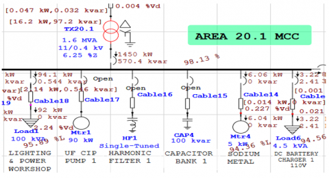
Scenario 2c; The same as scenario2a with the lack of Capacity bank2 100 kVar and Harmonic filter2 105 kVar (see Figure 7).
Note that the color of the transformer changes (red) after the simulation. It is very dangerous because the transformer is very overloaded, the upstream circuit breaker is tripped by protection to avoid damaging the transformer despite the shutdown of production, due to the increase of the current from 2126 to 2292A (166A) with an increase of more than 300% of the reactive power (kVar) from 177.2 to 570.4 and consequently a decrease of the power factor by 6.14% (99.2% to 93.06%) and the busbar voltage 14, 400 V by 1.64% (99.73% to 98.13%).
We conclude that the role of capacitor banks and harmonic filters is not only to guarantee a good quality of energy and to save in the electricity factor by compensating reactive energy and minimizing losses [18] but also to obtain more capacity for existing electrical equipment such as our transformer case, to increase their lifespan and to guarantee the continuity of production.
Scenario 3: During the power flow, the total power consumed is 4.73 MW, 1.135 MVar with a power factor is 96.35% (see Table 4);
No critical conditions with a good factor due to the capacitor bank, harmonic filter, and low load.
Scenario 4: In case of total absence of power supply from Sonelgaz, the diesel unit provides the necessary electrical energy to supply the emergency loads of the essential main switchboard after opening the normal circuit breakers and closing the essential circuit breakers automatically or manually according to the choice, and after simulation of the power flow (see Figure 5) and even in reality, not of the observed problem.
It is noted that in this plant (24/24h operation) there is no voltage drop (+/- 10%). which disrupts the quality of the electrical to stabilize the network by maintaining a quasi-constant voltage of the HTA busbar sets (11 kV) according to the evolution of the loads and fluctuations of the upstream voltage, the On-Load Tap Changer (OLTC) installed on the 220/11 kV transformer is an electromechanical system that adjusts the transformation ratio by adding or removing a number of control turns in series with the turns of the high-voltage winding (220 kV).
Table 5. The power loss with N and N-1 of full and low load scenario
|
Scenario |
Losses with N |
Losses with N-1 |
||
|
Active |
Reactive |
Active |
Reactive |
|
|
(kW) |
(kVar) |
(kW) |
(kVar) |
|
|
Full load |
647.4 |
4367.3 |
718.4 |
6666 |
|
Low load |
146.6 |
468.2 |
162 |
639.4 |
Table 5 shows the influence of the choice of contingency on the total active and reactive losses with the same load (full load or low load). The increase in active and reactive losses at full load N-1 (Scenario 2) compared to full load N (Scenario 1) is important, which explains the voltage drop in Scenario 2 compared to Scenario 1 and the same remark for low load N-1 compared to low load N.
After a series of simulations of the load flow analysis, if we make a comparison between the four scenarios that we have proposed (the most probable’s) we conclude that scenario1 is the most economical because it contains;
3.2 Simulation of short circuit analysis
The simulation of three-phase bolted three-phase short-circuits currents per IEC 60909 Standard. This study calculates initial symmetrical RMS, peak, symmetrical and asymmetrical breaking RMS, steady-state RMS short circuit currents and their DC offset at faulted nozzles as the basic system reference quantities approved in our previous article with a maximum value recorded in a three-phase bolted fault and defined as a model to be used and compared with the values obtained by the factory manufacturer with Different Load and Contingency Scenarios [19], all the important busses and those to be protected by main circuit breakers have been chosen as it allows the maximum current during the fault to be determined to determine the breaking and closing powers of the devices as well as the electromechanical and thermal behavior of the equipment of the devices and to calculate the settings of the protection relays and the fuse ratings, to ensure good selectivity [20-22].
Scenario 1: After the simulation (Table 6), it can be seen that all the fault values of the three-phase short circuit Ik of the main base and high voltage buses of each area of this HV customer are lower than the fault current obtained by the manufacturer, therefore it can be concluded that the circuit breakers are well dimensioned and capable of protecting the circuit against any type of fault for this scenario.
Scenario 2: To better interpret these results, we have broken down the buses into two parts A and B according to the voltage level:
A/High and medium voltage buses (220/11 kV): All the values of the three-phase short-circuit currents are lower than the results obtained in the scenario1 so all the circuit breakers are well dimensioned for this case.
Table 6. Short circuit analysis” 3-Phase fault with scenario 1
|
ETAP Results |
By Builder |
||||
|
ID |
Voltage kV |
I"k (kA) |
Ip (kA) |
Ik (kA) |
Icc (kA) |
|
Bus2 |
220 |
3,002 |
4,956 |
2,624 |
31.5 |
|
Bus4 |
11 |
26,747 |
56,637 |
20,838 |
31.5 |
|
Bus7 |
11 |
25,394 |
52,757 |
19,938 |
31.5 |
|
Bus14 |
0.4 |
45,537 |
100,947 |
37,461 |
50 |
|
Bus105 |
11 |
26,235 |
55,191 |
20,454 |
31.5 |
|
Bus117 |
0.4 |
53,873 |
120,458 |
46,111 |
50 |
|
Bus156 |
11 |
26,293 |
55,312 |
20,548 |
31.5 |
|
Bus185 |
0.4 |
43,179 |
96,931 |
37,537 |
50 |
|
Bus202 |
0.4 |
63,600 |
142,232 |
56,447 |
65 |
|
Bus220 |
11 |
26,503 |
55,937 |
20,663 |
31.5 |
|
Bus233 |
0.4 |
64,044 |
143,241 |
56,489 |
65 |
|
Bus266 |
11 |
26,40525 |
55,6373 |
20,62475 |
31.5 |
|
Bus300 |
0.4 |
24,61454 |
49,5398 |
22,18335 |
50 |
Table 7. Short circuit analysis” 3-Phase fault” with scenario 2
|
ETAP Results |
By Builder |
||||
|
ID |
Voltage kV |
I"k (kA) |
Ip (kA) |
Ik (kA) |
Icc (kA) |
|
Bus2 |
220 |
1,705 |
4,171 |
1,312 |
31.5 |
|
Bus4 |
11 |
20,663 |
60,455 |
14,198 |
31.5 |
|
Bus7 |
11 |
23,656 |
56,348 |
13,816 |
31.5 |
|
Bus14 |
0.4 |
49,770 |
109,94 |
36,296 |
50 |
|
Bus105 |
11 |
24,341 |
59,107 |
14,037 |
31.5 |
|
Bus117 |
0.4 |
59,759 |
133,410 |
44,357 |
50 |
|
Bus156 |
11 |
24,313 |
59,009 |
14,077 |
31.5 |
|
Bus185 |
0.4 |
48,432 |
108,334 |
36,266 |
50 |
|
Bus202 |
0.4 |
69,940 |
156,613 |
53,841 |
65 |
|
Bus220 |
11 |
24,509 |
59,804 |
14,125 |
31.5 |
|
Bus233 |
0.4 |
73,184 |
162,421 |
53,879 |
65 |
|
Bus266 |
11 |
24,393 |
59,343 |
14,109 |
31.5 |
|
Bus300 |
0.4 |
27,380 |
54,738 |
21,798 |
50 |
B/ Low voltage buses (400 V): All the values of the three-phase short-circuit currents are higher than the results obtained in the scenario 1 and the fault values for the three buses (bus 117, bus 202, and bus 233) are even higher than the result obtained by the manufacturer.
Bus 117 of MCC30.2 (area 30A): It can be seen that the three-phase short-circuit current Ik=59,759 kA is higher than the 50 kA current set by the manufacturer, but it is still lower than the breaking capacity of the 65 kA circuit breaker on the supply side of this bus and that this circuit breaker can protect the electrical circuit in case of a fault.
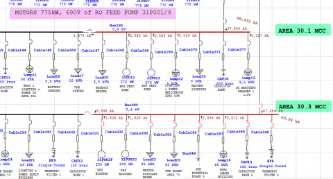
Bus 202 of MCC30.3 (area 30B): It can be seen that the three-phase short-circuit current Ik=69.94 kA (see Figure 8)is higher than the 65 kA current set by the manufacturer motion current and even higher than the breaking capacity of the 65 kA circuit breaker upstream of this bus and that this circuit breaker is not capable of protecting the electrical circuit in the event of a fault (see Table 9), but it is necessary to reduce the load by loads that do not affect production such as (HVAC Admin building 65 kVA, Water Service Motor 18 kW, RO CIP2 Motor 132 kW) and after the simulation, the value will decrease so that the circuit breaker can protect the circuit.
Bus 233 of MCC30.4 (area 30C): It can be seen that the three-phase short-circuit current Ik=73,184 kA is higher than the current of 65 kA and even higher than the breaking capacity of the 65 kA circuit breaker upstream of this bus, and that this circuit breaker is not able to protect the electric circuit in case of a fault (see Table 7). In case the load is reduced by loads that do not affect production, and after the simulation, the value is reduced but it is still higher than the breaking capacity of the circuit breaker because the margin is important.
Scenario 3: After the simulation, it can be seen that all fault values of the three-phase short circuit Ik of the main base and high voltage buses and each zone of the HV customer are lower than the fault currents of scenario 1, so it can be concluded that the circuit breakers are well dimensioned and capable of protecting the circuit against any type of fault and that the load has an influence on the value of the short circuit.
Table 8 represents a report of the three-phase short circuit of low voltage bus 202 & 233 with scenarios 2 which gives the maximum values of the fault and compare with all device capacity concerned (magnetic & thermal) to make an efficient and quick check to display all the overload alarms or a wrong dimensioning of the protection devices concerned are displayed on the study report.
Table 8. Short circuit report of “low voltage bus 202 & 233” with scenarios 2
|
Short-Circuit Summary Report |
||||||||||||
|
Bus |
Device |
Device Capacity (kA) |
Short-Circuit Current (kA) |
|||||||||
|
ID |
kV |
ID |
Type |
Peak |
Ib sym |
Ib asym |
I ’’k |
ip |
Ib sym |
Ib asym |
Idc |
Ik |
|
Bus202 |
0.400 |
Bus202 |
Bus |
154.0 |
70.0 |
70.218 |
69.939 |
156.612 |
64.299 |
64.859 |
8.506 |
53.841 |
|
|
0.400 |
Q3.MCC1 |
CB |
154.0 |
65.0 |
65.202 |
69.939 |
156.612 |
64.299 |
64.859 |
8.506 |
|
|
|
0.400 |
Q3.MCC2 |
CB |
154.0 |
50.0 |
50.034 |
69.939 |
156.612 |
64.299 |
64.859 |
8.506 |
|
|
|
0.400 |
CB30B.23 |
CB |
154.0 |
50.0 |
50.034 |
69.939 |
156.612 |
64.299 |
64.859 |
8.506 |
|
|
|
0.400 |
CB30B.24 |
CB |
154.0 |
70.0 |
70.218 |
69.939 |
156.612 |
64.299 |
64.859 |
8.506 |
|
|
|
0.400 |
CB30B.25 |
CB |
154.0 |
70.0 |
70.218 |
69.939 |
156.612 |
64.299 |
64.859 |
8.506 |
|
|
|
0.400 |
CB30B.26 |
CB |
154.0 |
70.0 |
70.218 |
69.939 |
156.612 |
64.299 |
64.859 |
8.506 |
|
|
|
0.400 |
CB30B.27 |
CB |
154.0 |
70.0 |
70.218 |
69.939 |
156.612 |
64.299 |
64.859 |
8.506 |
|
|
|
0.400 |
CB30B.28 |
CB |
154.0 |
70.0 |
70.218 |
69.939 |
156.612 |
64.299 |
64.859 |
8.506 |
|
|
|
0.400 |
CB30B.29 |
CB |
154.0 |
70.0 |
70.218 |
69.939 |
156.612 |
64.299 |
64.859 |
8.506 |
|
|
|
0.400 |
CB30B.30 |
CB |
154.0 |
70.0 |
70.218 |
69.939 |
156.612 |
64.299 |
64.859 |
8.506 |
|
|
Bus233 |
0.400 |
Bus233 |
Bus |
|
|
|
73.114 |
162.291 |
|
|
|
53.879 |
|
|
0.400 |
Q4.MCC1 |
CB |
154.0 |
70.0 |
70.218 |
73.114 |
162.291 |
66.809 |
67.349 |
8.510 |
|
|
|
0.400 |
Q4.MCC2 |
CB |
154.0 |
70.0 |
70.218 |
73.114 |
162.291 |
66.809 |
67.349 |
8.510 |
|
|
|
0.400 |
CB30C.14 |
CB |
154.0 |
50.0 |
50.034 |
73.114 |
162.291 |
66.809 |
67.349 |
8.510 |
|
|
|
0.400 |
CB30C.15 |
CB |
154.0 |
70.0 |
70.218 |
73.114 |
162.291 |
66.809 |
67.349 |
8.510 |
|
|
|
0.400 |
CB30C.16 |
CB |
154.0 |
70.0 |
70.218 |
73.114 |
162.291 |
66.809 |
67.349 |
8.510 |
|
|
|
0.400 |
CB30C.17 |
CB |
154.0 |
70.0 |
70.218 |
73.114 |
162.291 |
66.809 |
67.349 |
8.510 |
|
|
|
0.400 |
CB30C.18 |
CB |
154.0 |
70.0 |
70.218 |
73.114 |
162.291 |
66.809 |
67.349 |
8.510 |
|
|
|
0.400 |
CB30C.19 |
CB |
154.0 |
70.0 |
70.218 |
73.114 |
162.291 |
66.809 |
67.349 |
8.510 |
|
|
|
0.400 |
CB30C.20 |
CB |
154.0 |
70.0 |
70.218 |
73.114 |
162.291 |
66.809 |
67.349 |
8.510 |
|
|
|
0.400 |
CB30C.21 |
CB |
154.0 |
70.0 |
70.218 |
73.114 |
162.291 |
66.809 |
67.349 |
8.510 |
|
|
|
0.400 |
CB30C.22 |
CB |
154.0 |
50.0 |
50.034 |
73.114 |
162.291 |
66.809 |
67.349 |
8.510 |
|
|
|
0.400 |
CB30C.23 |
CB |
154.0 |
70.0 |
70.218 |
73.114 |
162.291 |
66.809 |
67.349 |
8.510 |
|
|
|
0.400 |
CB30C.24 |
CB |
154.0 |
50.0 |
50.034 |
73.114 |
162.291 |
66.809 |
67.349 |
8.510 |
|
|
|
0.400 |
CB30C.25 |
CB |
154.0 |
70.0 |
70.218 |
73.114 |
162.291 |
66.809 |
67.349 |
8.510 |
|
|
|
0.400 |
CB30C.28 |
CB |
154.0 |
70.0 |
70.218 |
73.114 |
162.291 |
66.809 |
67.349 |
8.510 |
|
|
ID |
Device Capacity |
3-Phase Short-Circuit Duty Result |
||||||
|
Bus ID |
Device ID |
Ithr(kA) |
Tkr(sec) |
Rated Thermal Energy (MJ) |
Ith (kA) |
Tkr(sec) |
Thermal Energy (MJ) |
|
|
Bus 202 |
Q3.MCC1 |
70.000 |
1.00 |
4900.00 |
64.324 |
1.20 |
4137.59 |
|
|
Bus 202 |
Q3.MCC3 |
65.000 |
1.00 |
4224.00 |
64.324 |
1.20 |
4137.59 |
|
|
Bus 202 |
CB.30B.23 |
50.000 |
1.00 |
2500.00 |
64.324 |
1.00 |
4137.59 |
|
|
Bus 202 |
CB.30B.24 |
50.000 |
1.00 |
2500.00 |
64.324 |
1.00 |
4137.59 |
|
|
Bus 202 |
CB.30B.25 |
70.000 |
1.00 |
4900.00 |
64.324 |
1.00 |
4137.59 |
|
|
Bus 202 |
CB.30B.26 |
70.000 |
1.00 |
4900.00 |
64.324 |
1.00 |
4137.59 |
|
|
Bus 202 |
CB.30B.27 |
70.000 |
1.00 |
4900.00 |
64.324 |
1.00 |
4137.59 |
|
|
Bus 202 |
CB.30B.28 |
50.000 |
1.00 |
2500.00 |
64.324 |
1.00 |
4137.59 |
|
|
Bus 202 |
CB.30B.29 |
50.000 |
1.00 |
2500.00 |
64.324 |
1.00 |
4137.59 |
|
|
Bus 202 |
CB.30B.30 |
70.000 |
1.00 |
4900.00 |
64.324 |
1.00 |
4137.59 |
|
|
Bus 233 |
Q4.MCC3 |
70.000 |
1.00 |
4900.00 |
66.376 |
1.00 |
4405.79 |
|
|
Bus 233 |
Q4.MCC1 |
70.000 |
1.00 |
4900.00 |
66.376 |
1.00 |
4405.79 |
|
|
Bus 233 |
CB.30C.14 |
50.000 |
1.00 |
2500.00 |
66.376 |
1.00 |
4405.79 |
|
|
Bus 233 |
CB.30C.15 |
70.000 |
1.00 |
4900.00 |
66.376 |
1.00 |
4405.79 |
|
|
Bus 233 |
CB.30C.16 |
70.000 |
1.00 |
4900.00 |
66.376 |
1.00 |
4405.79 |
|
|
Bus 233 |
CB.30C.17 |
70.000 |
1.00 |
4900.00 |
66.376 |
1.00 |
4405.79 |
|
|
Bus 233 |
CB.30C.18 |
70.000 |
1.00 |
4900.00 |
66.376 |
1.00 |
4405.79 |
|
|
Bus 233 |
CB.30C.19 |
70.000 |
1.00 |
4900.00 |
66.376 |
1.00 |
4405.79 |
|
|
Bus 233 |
CB.30C.20 |
70.000 |
1.00 |
4900.00 |
66.376 |
1.00 |
4405.79 |
|
|
Bus 233 |
CB.30C.21 |
70.000 |
1.00 |
4900.00 |
66.376 |
1.00 |
4405.79 |
|
|
Bus 233 |
CB.30C.22 |
50.000 |
1.00 |
2500.00 |
66.376 |
1.00 |
4405.79 |
|
|
Bus 233 |
CB.30C.23 |
70.000 |
1.00 |
4900.00 |
66.376 |
1.00 |
4405.79 |
|
|
Bus 233 |
CB.30C.24 |
50.000 |
1.00 |
2500.00 |
66.376 |
1.00 |
4405.79 |
|
|
Bus 233 |
CB.30C.25 |
70.000 |
1.00 |
4900.00 |
66.376 |
1.00 |
4405.79 |
|
|
Bus 233 |
CB.30C.28 |
70.000 |
1.00 |
4900.00 |
66.376 |
1.00 |
4405.79 |
|
|
ip is calculated using method C. |
LV CB duty determined based on service rating. |
|||||||
|
Ib does not include decay of non-terminal faulted induction motors. |
Total through current is used for device duty. |
|||||||
|
Ik is the maximum steady state fault current. |
|
|||||||
|
Idc is based on X/R from Method C and Ib as specified above. |
|
|||||||
|
* Indicates a device with calculated duty exceeding the device capability. # Indicates a device with calculated duty exceeding the device marginal limit. (95 % times device capability). |
||||||||
Figure 8. Short circuit analysis of “low voltage bus 185 & 202” with scenarios 2 (Area 30B)
Table 9. Short circuit analysis” 3-Phase fault” with scenario 3
|
ETAP Results |
By Builder |
||||
|
ID |
Voltage kV |
I"k (kA) |
Ip (kA) |
Ik (kA) |
Icc (kA) |
|
Bus2 |
220 |
2,718 |
6,688 |
2,624 |
31,5 |
|
Bus4 |
11 |
20,455 |
53,460 |
19,457 |
31,5 |
|
Bus7 |
11 |
19,600 |
49,854 |
18,751 |
31,5 |
|
Bus14 |
0,4 |
39,770 |
89,534 |
37,276 |
50 |
|
Bus105 |
11 |
20,126 |
51,901 |
19,158 |
31,5 |
|
Bus117 |
0,4 |
48,327 |
110,759 |
45,830 |
50 |
|
Bus156 |
11 |
20,208 |
52,285 |
19,232 |
31,5 |
|
Bus185 |
0,4 |
37,546 |
86,362 |
37,350 |
50 |
|
Bus202 |
0,4 |
59,387 |
136,048 |
56,027 |
65 |
|
Bus220 |
11 |
20,313 |
52,779 |
19,321 |
31,5 |
|
Bus233 |
0,4 |
56,488 |
130,502 |
56,068 |
65 |
|
Bus266 |
11 |
20,272 |
52,589 |
19,291 |
31,5 |
|
Bus300 |
0,4 |
23,428 |
47,721 |
22,147 |
50 |
This document shows that the operation of seawater desalination allows savings both in terms of total operating costs and payment of electricity bills. To allow the study, the scenario methodology chosen and developed the most probable, external, and critical cases, thus taking into account the uncertainties involved in the planning.
Using ETAP software, an analysis of the power flow and short-circuit of the distribution network of an HV customer operating 24 hours a day is carried out to detect weak points and check;
To the end that this industrial electrical system to meet the performance criteria and to ensure the following objectives;
Finally, we conclude that the methodology of this study is an electrical footprint of a facility's electricity consumption patterns, which provides key information, that the interpretation of this footprint is more than a science (technical skills), it is also an art (interpretive skills) and that scenario 1 is the most optimal considering not only the technical aspects of the issue, but also the economic aspects (save total operating and electricity bills in the future) because it has;
[1] Esmaeilion, F. (2020). Hybrid renewable energy systems for desalination. Applied Water Science, 10(3): 1-47. https://doi.org/10.1007/s13201-020-1168-5
[2] Bognar, K., Blechinger, P., Behrendt, F. (2012). Seawater desalination in micro grids: An integrated planning approach. Energy, Sustainability and Society, 2(1): 1-12. https://doi.org/10.1186/2192-0567-2-14
[3] Timalsena, K.R., Karki, R., Piya, P., Bhattarai, S. (2020). Need-based reliability investment in industrial/commercial power distribution systems. International Journal of System Assurance Engineering and Management, 11(3): 747-754. https://doi.org/10.1007/s13198-020-00998-5
[4] Ghiasi, M., Ghadimi, N., Ahmadinia, E. (2019). An analytical methodology for reliability assessment and failure analysis in distributed power system. SN Applied Sciences, 1(1): 1-9. https://doi.org/10.1007/s42452-018-0049-0
[5] Price, L., Wang, X., Yun, J. (2010). The challenge of reducing energy consumption of the Top-1000 largest industrial enterprises in China. Energy Policy, 38(11): 6485-6498. https://doi.org/10.1016/j.enpol.2009.02.036
[6] Nebey, A.H. (2020). Automatic load sharing of distribution transformer for overload protection. BMC Research Notes, 13(1): 1-6. https://doi.org/10.1186/s13104-019-4880-1
[7] Chafai, M., Refoufi, L., Bentarzi, H. (2016). Large power transformer reliability modeling. International Journal of System Assurance Engineering and Management, 7(1): 9-17. https://doi.org/10.1007/s13198-014-0261-2
[8] Jyothi, G., Yemula, P.K. (2017). Reactive Power Support from End Customer Equipment. Technology and Economics of Smart Grids and Sustainable Energy, 2(1): 1-7. https://doi.org/10.1007/s40866-017-0030-9
[9] Gamboa, R.A., Aravind, C.V., Chin, C.A. (2018). System Protection Coordination Study for Electrical Distribution System. In 2018 IEEE Student Conference on Research and Development (SCOReD), pp. 1-6. https://doi.org/10.1109 / SCORED. 2018.8710793
[10] Nepomnyashchiy, V.A. (2015). Electrical network reliability and system blackout development simulations. Thermal Engineering, 62(14): 993-1007. https://doi.org/10.1134/S0040601515140104
[11] Zeggai, A., Benhamida, F. (2019). Power flow and Short circuit of a Real Eectrolysis Plant. In 2019 Algerian Large Electrical Network Conference (CAGRE). https://doi.org/10.1109/CAGRE.2019.8713314
[12] Ramesh, L., Chakraborty, N. (2019). Optimal allocation of transformer and its effects on distribution system loss minimization. Russian Electrical Engineering, 90(3): 285-293. https://doi.org/10.3103/S1068371219030143
[13] Zeggai, A., Benhamida, F. (2019). Power flow and Short circuit of 220 kV Substation using ETAP. In 2019 Algerian Large Electrical Network Conference (CAGRE). https://doi.org/10.1109/CAGRE.2019.8713172
[14] Hashemi, F., Alizade, A.R., Zebardast, S.J., Ghadimi, N. (2011). Determining the optimum cross-sectional area of the medium voltage feeder for loss reduction and voltage profile improvement based on particle swarm algorithm. In 2011 10th International Conference on Environment and Electrical Engineering, pp. 1-5. https://doi.org/10.1109/EEEIC.2011.5874736.
[15] Lakra, N.S., Prakash, P., Jha, R.C. (2017). Power quality improvement of distribution system by reactive power compensation. In 2017 International Conference on Power and Embedded Drive Control (ICPEDC), pp. 415-420. https://doi.org/10.1109/ICPEDC.2017.8081125
[16] Mandefro, E., Bantiyrga, B. (2019). Optimal allocation of distributed generation for performance enhancement of distribution system using particle swarm optimization. In International Conference on Advances of Science and Technology, 308: 436-453. https://doi.org/10.1007/978-3-030-43690-2_30
[17] Kurian, S.C., Kumar, K.N. (2017). Relay co-ordination in a 11kV substation using ETAP. In International Journal of Recent Innovation in Engineering and Research Scientific Journal.
[18] Pico, J.D., Celeita, D., Ramos, G. (2016). Protection coordination analysis under a real-time architecture for industrial distribution systems based on the Std IEEE 242-2001. IEEE Transactions on Industry Applications, 52(4): 2826-2833. https://doi.org/10.1109/TIA.2016.2538739
[19] Thangalakshmi, S. (2016). Planning and coordination of relays in distribution system. Indian Journal of Science and Technology, 9(31): 1-7. https://doi.org/10.17485/ijst/2016/v9i31/91734
[20] Kamel, S., Shaban, A., Korashy, A., Nasrat, L., Yu, J., Wang, S. (2019). Short circuit analysis and coordination of overcurrent relays for a realistic substation located in upper Egypt. In 2019 IEEE Innovative Smart Grid Technologies-Asia (ISGT Asia), pp. 2150-2155. https://doi.org/10.1109/ISGT-Asie.2019.8881785
[21] Juamperez, M., Yang, G., Kjær, S.B. (2014). Voltage regulation in LV grids by coordinated volt-var control strategies. Journal of Modern Power Systems and Clean Energy, 2(4): 319-328. https://doi.org/10.1007/s40565-014-0072-0
[22] Li, R., Wong, P., Wang, K., Li, B., Yuan, F. (2020). Power quality enhancement and engineering application with high permeability distributed photovoltaic access to low-voltage distribution networks in Australia. Protection and Control of Modern Power Systems, 5(1): 1-7. https://doi.org/10.1186/s41601-020-00163-x
[23] Nebey, A.H. (2020). Automatic load sharing of distribution transformer for overload protection. BMC Research Notes, 13(1): 1-6. https://doi.org/10.1186/s13104-019-4880-1
[24] Ovaere, M., Heylen, E., Proost, S., Deconinck, G., Van Hertem, D. (2019). How detailed value of lost load data impact power system reliability decisions. Energy Policy, 132: 1064-1075. https://doi.org/10.1016/j.enpol.2019.06.058