Sukanta Patra | Prasenjit Sarkhel | Nirmal Baran Hui* | Nilotpal Banerjee
© 2020 IIETA. This article is published by IIETA and is licensed under the CC BY 4.0 license (http://creativecommons.org/licenses/by/4.0/).
OPEN ACCESS
In this work, the modeling of a single-link flexible manipulator has been done using simmechanics tool of Matlab and treated as a fishing rod. An elastic string is attached to the free end of the rod. A payload is given to the open end of the string for the deflection analysis of the flexible rod. The simmechanics model of the flexible rod has been developed using the lumped parameter approach. Initially, the developed modeling technique has been validated by comparing the deflection obtained from the proposed model simulation and the conventional formulae with particular payload at the free end. Later on, to attain the fishing rod-like structure, the cross-section of the rod has been made taper towards its open end. Then, different loading conditions have been applied to the free end of the string, and the model behavior has been studied. Results obtained from the simulated model are presented and discussed under all the loading conditions.
flexible rod, simmechanics model, deflection, lumped parameter approach
Flexible manipulators are preferred over rigid ones due to the following reasons: lightweight, low power consumption, requirement of small actuators and greater maneuverability as well as transportability, less expensive and large payload to mass ratio. However, control of flexible manipulator is a difficult job because it succumbs high vibration. For which, proper system models and useful controllers are required. The primary objective of this paper is to develop such a flexible manipulator system and control it.
Many modeling techniques are available in the literature; some of them are mentioned below with their pros and cons. Khalil et al. [1] presented a lumped parameter approach. This technique has found its application in high-speed machine tools and robots with elastic joints. For a given point to point task, Yue et al. [2] have established the maximum dynamic payload carrying capacity of a flexible redundant robot manipulator. In this work, the flexible manipulator system dynamics has been developed using the finite element method. But, it is a mathematically very cumbersome approach, and computational complexity is very high. Mohamed et al. [3] presented some control strategies for the manipulator system with high flexibility to control its excessive vibration. The dynamic analysis of the manipulator systems with flexibility has been surveyed by Dwivedy et al. [4]. Here, link and joints are considered as flexible, and an investigation has been done to thoroughly examine the techniques and methodologies used in these analyses, their advantages and the possible outcomes. Macchelli et al. [5] presented a linear quadratic regulator-based method to model robotic links incorporating flexibility. Vakil et al. [6] introduced a different controlling technique to track the position of the end-effector of multiple link manipulators considering the flexibility. A robust controller has been developed by Khairudin et al. [7].
Bian et al. [8] have suggested a method to suppress the impact vibration of the flexible manipulator using its structural characteristic when capturing a moving object. Shawky et al. [9] developed a model for a single-link flexible manipulator and suggested a control scheme for the tip position control. An inclusive focus has been paid by Sayahkarajy et al. [10] to model and controls a two-link flexible manipulator. Accounts for huge deflections in three-dimensional spaces. An approach to modelling flexible manipulators consisting of rotary joints and flexible links has been proposed by Konno et al. [11]. Yoshikawa et al. [12] have discussed a distributed state estimation method which uses discrete position information of markers attached on flexible links. An improved efficiency dynamic modelling method using lumped parameter based Holzer method has been proposed by Ding and Selig [13]. Pereira et al. [14] have proposed a method to modify the dynamics of single-link flexible arms in order to allow the design of a control system which is more robust to changes in the payload value. Different systematic methods for efficient modelling and dynamics computation of flexible robot manipulators have been developed by Li et al. [15] using the Lagrangian assumed modes method. Lee [16] has geometrically derived differential kinematics of a flexible manipulator to calibrate model parameters such as the D‐H parameters, the joint compliances and the mass positions. The global mode method (GMM) has been proposed by Wei et al. [17] to obtain a reduced-order analytical dynamic model for a signal flexible-link flexible-joint (SFF) manipulator. Meng et al. [18] have derived the rigid-flexible coupling dynamics of a space robot system with flexible appendages and have established a coupling model between the flexible base and the space manipulator. Lagrange dynamics differential equations of the two-link flexible robot manipulator have been established by Zhang et al. [19] using the integrated modal method and the multi-body system dynamics method. A new program method for the generation of efficient kinematic and dynamic flexible robot models has been described by Surdilovic et al. [20]. Ouyang et al. [21] have investigated the reinforcement learning control of a single link flexible manipulator and have attempted to suppress the vibration due to its flexibility and lightweight structure. Modelling and vibration of a flexible link manipulator with tow flexible links and rigid joints have been investigated by Abedi et al. [22] which can include an arbitrary number of flexible links. The vibration control of single- link flexible manipulators with a payload has been studied numerically and experimentally by Malgaca et al. [23]. Mahto et al. [24] have used finite element method based on Lagrangian formulation for obtaining the equations of motion of the double link flexible revolute-jointed robotic manipulator. Kumar et al. [25] have made a noteworthy attempt to demonstrate brief modelling of N-link manipulator and subsequent modal characterization along with the determination of static deflection of a two-link flexible manipulator with a payload.
However, all the developed models have their limitations on considering both links as well as joint flexibilities, gravitational and frictional effects and deriving dynamic solution of a large number of DOFs. It is also sure to say that accurate control of such systems become very difficult until or unless system dynamic equations are properly known/derived. Therefore, there is still a need to develop a robust controller for attenuating flexible manipulators. Thus, in this research work, a flexible fishing rod has been modeled with the help of simmechanics. An elastic string carrying a payload is attached to the rod and behavior is studied. The structure of the paper is as follows: In Section 2, the construction of a flexible fishing rod has been discussed in the sim-mechanics environment. Here, to study the behavior of the system model in a real-life situation, different loading condition has been introduced to the model. Results and discussions have been elaborated in Section 3. In the end, conclusions are given in Section 4.
2.1 Lumped parameter
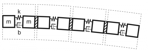
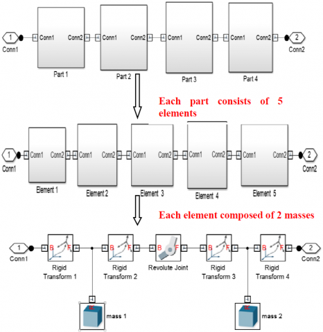
There are several methods available today to study flexible bodies [8]. In the present study, Matlab Simulink has been utilized to model the flexible link. As Simulink does not involve structural analysis, every element is considered as a rigid member. Further, to include flexibility, there are two approaches: the lumped parameter method and the finite element method. In this work, the lumped parameter method has been used. The link is approximated as a collection of discrete flexible units fixed to one another. Each flexible unit consists of two rigid mass elements connected through joint involving internal springs and dampers, as shown in Figure 1. The degree of freedom of the connection captures the deformation, and the spring and damper account for the stiffness and damping characteristics.
Figure 1. A flexible body according to lumped parameter method [26]
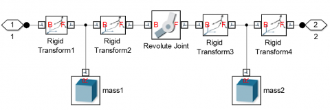
Modeling of a cantilever beam with rectangular cross-section has been shown in Figure 1. A flexible beam element considering steel material has been modeled in Matlab Simulink using simmechanics toolbox. The dimension and the material properties of the steel beam element are summarized in Table 1. The Simulink diagram of the flexible element has been shown in Figure 2.
Table 1. Dimension and properties of steel beam
|
Length(L) |
0.12m |
|
Width(w) |
0.02m |
|
Thickness(t) |
0.01m |
|
Density(den)-Aluminium |
7800kg/ m2 |
|
Young’s Modulus(E) |
210GPa |
|
Second Moment of area(I) |
1.667Χ10-9kgm2 |
Figure 2. Simulink diagram of a flexible cantilever beam element
The stiffness (k) of the revolute joint is calculated by the flexural formula K = $\frac{E I}{L}$ ; I= $\frac{w t^{3}}{12}$ .
$\mathrm{K}=\frac{210 \times 10^{9} \times \frac{0.02 \times 0.01^{3}}{12}}{0.12}=2.916 \times 10^{3} \mathrm{Nm} / \mathrm{rad}$
The damping coefficient (c) is taken as linear and proportional to stiffness (k) and calculated as $c=a \times K$ ; where, a is the proportional factor derived empirically and is related to the discretisations level of the beam. The value of spring stiffness and damping coefficient has been given in Table 2.
Value of a =3.4Χ10-5
So, c= $3.4 \times 10^{-5} \times 2.916 \times 10^{3}$ = $0.099144 \mathrm{Nm} /$$\left(\right.$rad $\left.\sec ^{-1}\right)$
Table 2. Values of spring stiffness and damping coefficient
|
Spring stiffness |
$2.916 \times 10^{2} \mathrm{Nm} / \mathrm{rad}$ |
|
Damping coefficient |
$0.099144 \mathrm{Nm} /\left(\mathrm{radsec}^{-1}\right)$ |
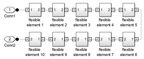
Figure 3. Simulink diagram of an overall cantilever beam with ten subsystems
Figure 4. Flexible beam model with a point load at a free end
The cantilever beam has been constructed using ten such elements, as shown in Figure 3-each part consisting of 2 rigid bodies coupled with a revolute joint, as shown in Figure 2. Cantilever boundary condition has been applied on the beam, and two different loading cases were studied for model validation purpose.
The Simulink diagram of the flexible beam model with payload is shown in Figure 4.
2.2 Description of the Simulink model
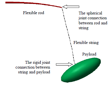
The Simulink model of the fishing rod consists of 3 essential elements, namely, flexible rod, flexible string, and payload, as shown in Figure 5. Simulink model of those three elements is described one after another in the subsequent sections.
Figure 5. A load pulls the flexible rod through a string
2.2.1 Flexible fishing rod
The flexible rod is made of steel with one of its ends fixed (resembling to a rod held at one end by someone or something) and behaving as a cantilever beam. The section of the rod along its length is tapered with a circular cross-section (refer to Figure 6). The whole rod is divided into four parts with smaller end radius being 20% lesser than the larger end radius for each component and presented in Table 3. The Simulink diagram of the above model is shown in Figure 7.
Table 3. Dimensions of the fishing rod
|
Length |
0.6m |
|
|
Length of each part |
0.6/4=0.15m |
|
|
Part no. |
Larger end radius |
Smaller end radius |
|
1 |
1.25cm |
1.0cm |
|
2 |
1.0cm |
0.8cm |
|
3 |
0.8cm |
0.64cm |
|
4 |
0.64cm |
0.512cm |
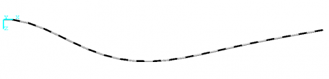
Figure 6. Flexible Link, 3D model
Here, K=EI/L, K= joint stiffness, I= $\pi r^{4} / 4$ , r = radius at the revolute joint connection.
C=A x K, A=proportional constant (2.55Χ10-5) C=Damping coefficient.
Each part of the rod is composed of five flexible elements and every element consisting of 2 masses coupled together by a revolute joint with stiffness and damping.
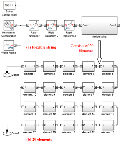
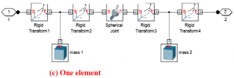
2.2.2 Flexible string
The flexible string (refer to Figure 8) is modeled using the same principle of the lumped parameter method. The string is used to establish a connection between the rod and the payload. It consists of 20 elements assembled via a rigid connection. Each part includes two masses of cylindrical shape coupled by a spherical joint that provide three rotational degrees of freedom to the joint. Hence, it can be simulated as a practical string of high flexibility. The material properties of the string are presented in Table 4.
Figure 7. Simulink model of the fishing rod
Table 4. Properties of flexible string material
|
Total Length |
80 cm |
|
Length of each element |
4 cm |
|
Cross-section diameter |
0.2048 cm |
|
Young’ Modulus (E) |
2.7GPa |
|
Density |
1150 kg/m2 |
|
Stiffness (K) |
93.2x10⁻² Nm/rad |
|
Damping coefficient(C) |
$4.823 \times 10^{-8} \mathrm{Nm} /\left(\mathrm{rad} \mathrm{sec}^{-1}\right)$ |
The Simulink diagram of the string is presented in Figure 9.
Figure 8. Flexible string
Payload has been connected to the rod through the flexible string to simulate the mass and movement of a fish trapped at the end of the string. The string is also subjected to a force (applied through payload) approximately in the plane normal to the axis of the string to model the movements of the fish trying to escape the trap.
The payload is considered as an ellipsoid of dimension mentioned in Table 5.
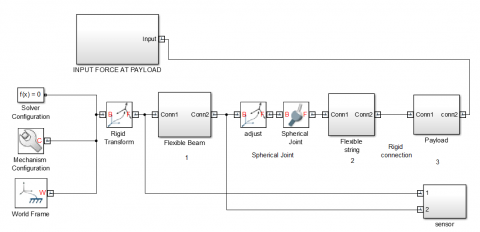
2.2.4 Assembly of the overall system
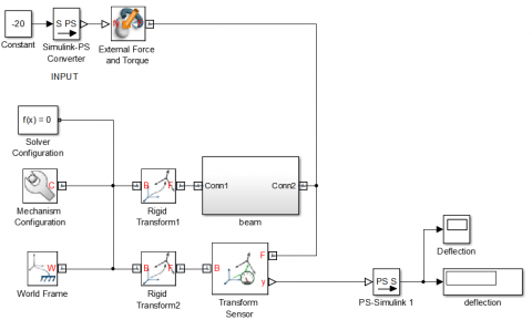
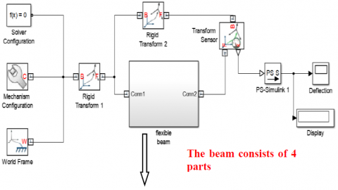
The final model of the fishing rod was obtained by assembling the flexible rod, flexible string and payload. Firstly, the flexible rod is fixed at one end, and the other end is attached to the string through a spherical joint (at the lower end at the circumference of cross-section of the rod). Secondly, the lower end of the string was attached to the payload (fish) via a rigid connection to develop the full model, as shown in Figure 10. After assembling the main parts, a solver, world frame, mechanism configuration (environment), a transform sensor(to measure the endpoint results of the flexible rod) are attached to simulate the model (refer to Figure 10).
Table 5. Radius (in cm) of Ellipsoids in three directions.
|
R1 |
25 |
|
R2 |
15 |
|
R3 |
10 |
|
Density |
700 kg/ m2 |
Figure 10. Simulink model of the complete system
The model is simulated in Matlab environment, and obtained results are presented and discussed in the subsequent sections.
3.1 Validation of the proposed model – rigid beam consideration
Two different loading conditions are considered in the present study.
Case I: Loaded under self-weight
The analytical deflection has been calculated by using the formula $y=\frac{w L^{4}}{8 E t}$ .
where, w= ( $\frac{m g}{L}$ ), g=9.81 m/s2.
The value of y has been obtained using the above formula as y=0.01133m.
From the model simulation, the ‘y’ value is found to be, y=0.01128m.
Case II: Point load at the free end (30N)
The deflection at the free end due to point load acting downwards is $y=\frac{w L^{3}}{3 E t}$ .
where, w=30N.
Here, the value of deflection has been obtained using the above formula as y=0.04936m.
The simulation result of the equilibrium deflection is found to be, y=0.04916m.
It can be concluded that the deflection values calculated from the conventional analytical formula are well in match with the values obtained from the simulation results. Thus, the modeling technique proposed in this work has been validated by comparing the above results.
3.2 The behaviour of a flexible fishing rod system with payload
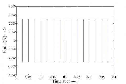
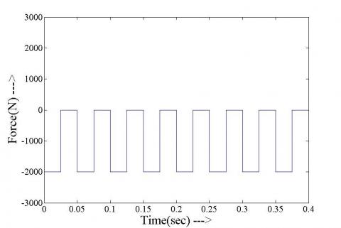
The complete system of the flexible fishing rod model has been simulated, and the simulation results have been plotted against time. A load of 2500N in a horizontal plane and a pulsating load of -2000N in a vertical plane have been applied. The loading curve in horizontal and vertical planes is shown in Figure 11.
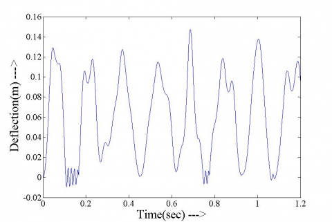
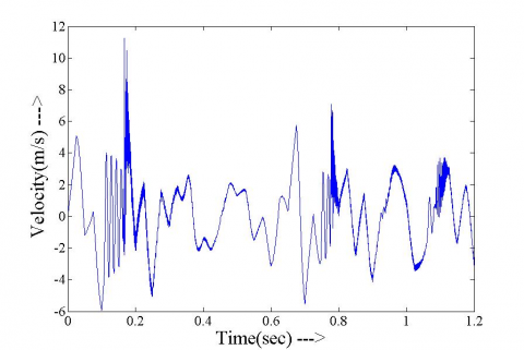
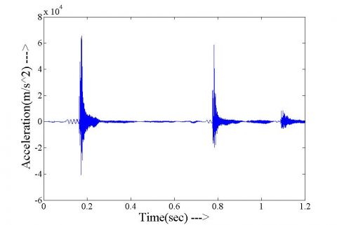
The plots of deflection, velocity and acceleration at the free end of the rod connected to string are shown in Figure 12. Deflections at the different instant of time are also presented in Table 6, and maximum deflection is found to be 0.15m.
Table 6. Deflection at a free end
|
Sl no |
Time(seconds) |
Deflection(m) |
Maximum deflection(m) |
|
1 |
0.15 |
0.1 |
0.15 |
|
2 |
0.30 |
0.032 |
|
|
3 |
0.45 |
0.02 |
|
|
4 |
0.60 |
0.04 |
|
|
5 |
0.75 |
0.03 |
(a)Horizontal Plane
(b) Vertical Plane
Figure 11. Applied Load (F) in horizontal and vertical planes
(a) Deflection vs. Time
(b) Velocity vs. Time
(c) Acceleration vs. Time
Figure 12. Deflection, velocity and acceleration at the free end of the flexible rod
3.3 Flexible fishing rod system subjected to different loading conditions
The dynamic behaviour of the flexible fishing rod system has been studied under different loading conditions. For studying the dynamic nature of the fishing rod in a real-life situation, two different loading conditions have been introduced at the free end of the flexible string.
3.3.1 Loading condition I
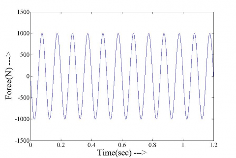
In this case, a sinusoidal load having 1000N amplitude and frequency of 62.832 rad/sec has been applied at the free end of the string. Load curve has been shown in Figure 13.
Figure 13. Load curve in a vertical direction
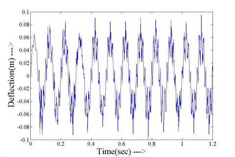
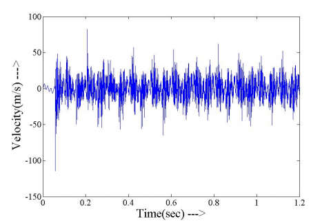
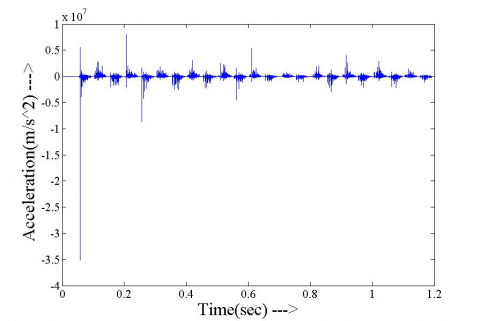
The Figure 14 illustrates the simulation result for the deflection, velocity and acceleration of the fishing rod under the said condition of loading and maximum deflection comes out to be 0.09 m (refer to Table 7).
Table 7. Deflection of the fishing rod under sinusoidal load at the free end of the string
|
Sl no. |
Time(seconds) |
Deflection(m) |
Maximum deflection(m) |
|
1 |
0.12 |
0.062 |
0.09 |
|
2 |
0.24 |
0.09 |
|
|
3 |
0.36 |
-0.09 |
|
|
4 |
0.48 |
-0.08 |
|
|
5 |
0.60 |
-0.025 |
(a) Deflection vs. Time
(b) Velocity vs. time
Figure 14. Deflection, velocity and acceleration at the free end of the flexible rod
In case of sinusoidal loading the tip responses shown in article was obtained as a result of combined effect of the flexible rod dynamics and applied loading. When the load increases sinusoidally in downward direction the tension in the string increases, this pulls the rod tip downwards and an increasing deflection is observed, but when the magnitude of the load decreases after attaining the peak and reverses, the tension in string also reduces and becomes zero until it is pulled in the upward direction due to sinusoidal load. As the tension falls in the string the vibration in the rod increases due to the flexible nature, with time when the tension in string builds up, the in the rod is pulled in that direction and the thing repeats. Hence it can be seen that the vibration is mostly obtained in the case where the load changes its direction or the tension in the string becomes zero.
3.3.2 Loading condition II
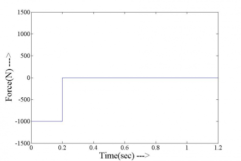
In this case, a sudden load of -1000 N for 0.2 sec has been applied at the free end of the string and withdrawn after that time. The loading curve is shown in Figure 15.
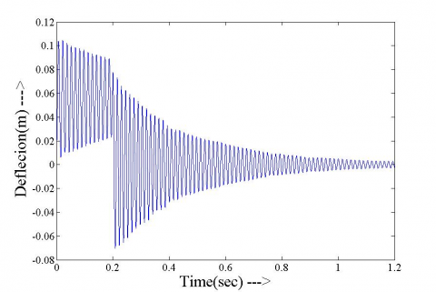
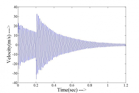
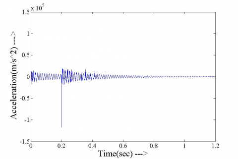
Figure 16 illustrates the simulation result for the deflection, velocity and acceleration of the fishing rod under this condition of loading and maximum deflection is obtained as 0.102m (refer to Table 8).
Under the application of sudden loading, a downward load is suddenly applied at the end of the string which pulls the flexible rod tip; this gives rise to vibration in the rod about a certain mean deflection, which is same as some weight hanging abruptly from the rod tip through a string. After a certain time when the load is removed suddenly, which is similar to the weight being accidentally detached from the string, the tension vanishes which induces larger vibration in the rod about the zero deflection position which is shown in the article. Further to get a better insight the velocity and acceleration were also generated for rod tip.
Table 8. Deflection of the fishing rod under sudden load at the free end of the string
|
Sl no |
Time(sec) |
Deflection(m) |
Maximum Deflection(m) |
|
1 |
0.01 |
0.102 |
0.102 |
|
2 |
0.1 |
0.092 |
|
|
3 |
0.2 |
0.075 |
|
|
4 |
0.35 |
0.04 |
|
|
5 |
0.55 |
-0.02 |
Figure 15. Load (F) applied in a vertical direction
(a) Deflection vs. time
(b) Velocity vs. Time
(c) Acceleration vs time
Figure 16. Deflection, velocity and acceleration at the free end of the flexible rod
In this work, a flexible fishing rod model has been developed using simmechanics platform of Matlab. At first, the developed modeling technique has been validated by comparing the deflection obtained from the proposed model simulation of a cantilever beam and the conventional formulae with specific payload at the free end. After that, to attain the fishing rod-like structure, a circular rod has been considered, and the cross-section of the rod is tapered towards its free end. Then, different loading conditions have been applied to the free end of the string, and the model behavior has been studied. In the end, all the results obtained from the model simulation have been presented and discussed under all the loading circumstances.
The simulation results indicate the presence of active vibration under all the loading conditions. Moreover, considering the real-life situation of the fishing system, a trajectory must be followed by the existing system model presented here and the control task will become more challenging. Therefore, proper control strategy must be introduced into the system model to serve for the above purpose. Presently, the authors are working toward those issues.
[1] Khalil, W., Gautier, M. (2000). Modeling of mechanical systems with lumped elasticity. Proceedings of the 2000 IEEE-International Conference on Robotics & Automation, San Francisco, CA, USA, USA. https://doi.org/10.1109/ROBOT.2000.845349
[2] Yue, S.G., Tso, S.K., Zu, W.L. (2001). Maximum dynamic payload trajectory for flexible robot manipulators with kinematic redundancy. Mechanism and Machine Theory, 36(6): 785-800. https://doi.org/10.1016/S0094-114X(00)00059-8
[3] Mohameda, Z., Martinsb, J.M., Tokhic, M.O., Sa da Costab, J., Botto, M.A. (2005). Vibration control of a very flexible manipulator system. Control Engineering Practice, 13(3): 267-277. https://doi.org/10.1016/j.conengprac.2003.11.014
[4] Dwivedy, S.K., Eberhard, P. (2006). Dynamic analysis of flexible manipulators, a literature review. Mechanism and Machine Theory, 41(7): 749-777. https://doi.org/10.1016/j.mechmachtheory.2006.01.014
[5] Macchelli, A., Melchiorriand, C., Stramigioli, S. (2007). Port-based modeling of a flexible link. IEEE Transactions on Robotics, 23(4): 650-660. https://doi.org/10.1109/TRO.2007.898990
[6] Vakil, M., Fotouhi, R., Nikiforuk, P.N. (2009). Maneuver control of the multilink flexible manipulators. International Journal of Nonlinear Mechanics, 44(8): 831-844. https://doi.org/10.1016/j.ijnonlinmec.2009.05.008
[7] Khairudin, M., Mohamed, Z., Husain, A.R. (2011). Dynamic model and robust control of flexible link robot manipulator. 9(2): 279-286. https://doi.org/10.1016/j.ijnonlinmec.2009.05.008
[8] Bian, Y.S., Gao, Z.H., Deng, Y.C. (2013). Impact vibration reduction for flexible manipulator via controllable local degrees of freedom. Chinese Journal of Aeronautics, 26(5): 1303-1309. https://doi.org/10.1016/j.cja.2013.04.010
[9] Shawky, A., Zydek, D., Elhalwagy, Y.Z., Ordys, A. (2013). Modeling and nonlinear control of a flexible link manipulator. Applied Mathematical Modeling, 37(23): 9591-9602. https://doi.org/10.1016/j.apm.2013.05.003
[10] Sayahkarajy, M., Mohamed, Z., Faudzi, A.A.M. (2016). Review of modelling and control of flexible link manipulators. Institue of Mechanical Engineers-Systems and Control Engineering, 230(8): 861-873. https://doi.org/10.1177%2F0959651816642099
[11] Konno, A., Uchiyama, M. (1996). Modeling of a flexible manipulator dynamicsbased upon holzer’s model. IEEE Conference, Osaka, Japan. https://doi.org/10.1109/IROS.1996.570675
[12] Yoshikawa, T., Ohta, A., Kanaoka, K. (2001). State estimation and parameter identification offlexible manipulators based on visual sensor and virtual joint model. IEEE-International Conference on Robotics &Automation, 2001. https://doi.org/10.1109/ROBOT.2001.933052
[13] Ding, X.L., Selig, J.M. (2004). Lumped parameter dynamic modeling for the flexible manipulator. IEEE-Proceedings of the 5thWorld Congress on Intelligent Control and Automation, Hangzhou, China. https://doi.org/10.1109/WCICA.2004.1340574
[14] Feliu, V., Pereira, E., Diaz, I.M., Roncero, P. (2006). Feedforward control of multimode single-link flexible manipulators based on an optimal mechanical design. ELSEVIER-Journal of Robotics and Autonomous Systems, 54(8): 651-666. https://doi.org/10.1016/j.robot.2006.02.012
[15] Li, C.J., Sankar, T.S. (1993). Systematic methods for efficient modeling anddynamics computation of flexible robot manipulators. IEEE Transactions on Systems, Man, and Cybernetics, 33(1): 77-95. https://doi.org/10.1109/21.214769
[16] Lee, B.J. (2013). Geometrical derivation of differential kinematics to calibrate model parameters of flexible manipulator. International Journal of Advanced Robotic Systems, 10-106. https://doi.org/10.5772/55592
[17] Wei, J., Cao, D.Q., Liu, L., Huang, W.H. (2017). Global mode method for dynamic modeling of a flexible-link flexible-joint manipulator with tip mass. ELSEVIER-Journal of Applied Mathematical Modelling, 48: 787-805. https://doi.org/10.1016/j.apm.2017.02.025
[18] Meng, D.S., Wang, X.Q., Xu, W.F., Liang, B. (2017). Space robots with flexible appendages: Dynamic modeling, coupling measurement, and vibration suppression. ELSEVIER- Journal of Sound and Vibration, 396: 30-50. https://doi.org/10.1016/j.jsv.2017.02.039
[19] Zhang, C.Y., Bai, G.C. (2012). Extremum response surface method of reliability analysis on two-link flexible robot manipulator. Publication of Central South University Press and Springer-Verlag Berlin Heidelberg, 19(1): 101-107. https://doi.org/10.1007/s11771-012-0978-5
[20] Surdilovic, D., Vukobratovic, M. (1996). One method for efficient dynamic modeling of flexible manipulators. ELSEVIER-Journal of Mechanisms and Machine Theory, 31(3): 297-315. https://doi.org/10.1016/0094-114X(95)00072-7
[21] Ouyang, Y.C., He, W., Li, X.J., Liu, J.K., Li, G. (2017). Vibration control based on reinforcement learning for a single link flexible robotic manipulator. Conference on IFAC Papers OnLine, 50(1): 3476-3481. https://doi.org/10.1016/j.ifacol.2017.08.932
[22] Abedi, E., Nadooshan, A.A., Salehi, S. (2008). Dynamic modeling of tow flexible link manipulators. World Academy of Science, Engineering and Technology, 2(10): 1140-1146. https://doi.org/10.5281/zenodo.1071658
[23] Malgaca, L., Yavuz, S., Akdag, M., Karagülle, H. (2016). Residual vibration control of a single-link flexible curved manipulator. ELSEVIER-Journal of Simulation Modelling Practice and Theory, 67: 155-170. https://doi.org/10.1016/j.simpat.2016.06.007
[24] Mahto, S., Dixit, U.S. (2014). Parametric study of double link flexible manipulator. Universal Journal of Mechanical Engineering, 2(7): 211-219. https://doi.org/10.13189/ujme.2014.020701
[25] Kumar, P., Pratiher, B. (2019). Modal characterization with nonlinear behaviours of a two-link flexible manipulator. Journal of Arch Applied Mechanics, 89: 1201-1220. https://doi.org/10.1007/s00419-018-1472-9
[26] Miller, S., Soares, T., Weddingen, Y., Wendlandt, J. (2017). Modeling Flexible Bodies with Simscape Multibody Software. TECHNICAL PAPER. © 2017 The MathWorks, Inc. MATLAB and Simulink are registered trademarks of The MathWorks, Inc.