Ravindranath Tagore Yadlapalli* | Anuradha Kotapati
© 2020 IIETA. This article is published by IIETA and is licensed under the CC BY 4.0 license (http://creativecommons.org/licenses/by/4.0/).
OPEN ACCESS
This paper presents the modeling and control of Air Breathing Fuel Cell (ABFC) and solar PV based power system for feeding the voltage regulator module of a laptop computer. The MATLAB modeling comprises of power sources as well as power conditioning units (PCUs). The different power sources under consideration are ABFC stack and solar PV module feeding the PCUs. The quadratic buck converter (QBC) and boost converter combination are used as a power conditioning unit (PCU). The average current mode control (ACMC) based QBC enables good steady state and dynamic voltage regulations. The perturb and observe (P&O) algorithm is used for maximum power tracking of solar PV panel. The efficiency analysis of ABFC power system and PV module power system are represented.
fuel cell, controllers, synchronous rectification (SR)
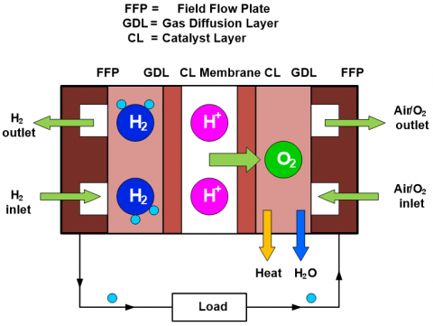
A Fuel Cell is an electrochemical device that produces electrical energy without the need of an intermediate stage [1-3]. It uses hydrogen in the electro-chemical reaction process and the byproducts are water, heat and electricity. The chemical reactions at anode and cathode are given by Eqns. (1)-(3).
$2 \mathrm{H}_{2} \rightarrow 4 \mathrm{H}^{+}+4 \mathrm{e}^{-}$ (1)
$\mathrm{O}_{2}+4 \mathrm{H}^{+}+4 \mathrm{e}^{-} \rightarrow 2 \mathrm{H}_{2} \mathrm{O}$ (2)
$2 \mathrm{H}_{2}+\mathrm{O}_{2} \rightarrow 2 \mathrm{H}_{2} \mathrm{O}+$ Electricity $+$ Heat (3)
The cells that extract oxygen from the ambient air through passive means for cathode reaction are named as “air-breathing” fuel cells [2]. In Air Breathing Fuel Cell (ABFC), the oxygen supply to cathode happens from free convection air flow whereas hydrogen to anode comes from compressed gas cylinders. The schematic of an ABFC is shown in Figure 1.
Figure 1. Schematic of ABFC
There is no need of auxiliary fan in ABFCs. This reduces the overall system volume and weight which is useful for laptop computer voltage regulator module (VRM) applications. Moreover, air is preferable than oxygen for curtailing the inflammable nature that is arising from hydrogen. A single ABFC typically achieves 0.5 V to 0.7 V. For electronic devices like laptops, which require relatively high power, a fuel cell stack is obtained by adding several cells in series. The Switched Mode Power Supplies (SMPS) are prominent because they have high packing density in addition to good efficiency. Recent advances in integrated circuitries demand for high conversion ratio’s from dc-dc converters to produce desired output voltages of 1 V, 1.5 V, 3.3 V and 12 V. The buck converter is not pertinent for such applications due to minimum turn-on time necessity of the switch. Its operation is also limited to lower dc-dc converter switching frequencies [4, 5]. On the other hand, cascade connection downside is the low efficiency even though it has a positive scope of achieving high conversion ratios. Therefore, the preferable one is the quadratic buck converter (QBC). On the other hand, it is always economical to use multiple sources of energy. This paper presents the ABFC and solar PV based power system for powering the laptop computer VRM. Here, the fuel cell is the primary source of energy and the solar power is used whenever it is available [6]. In ABFC power system, the QBC controls the unregulated output voltage of the ABFC fuel cell stack using average current mode control (ACMC) technique. The QBC converts 19 V obtained from the fuel stack to 1 V, acts as a laptop computer VRM. In PV power system the boost converter is used for maximum power tracking. The QBC converts the intermediate voltage level obtained at the output of boost converter to the desired voltage of 1 V. The paper organization is as follows; section 2 presents the overall view of the ABFC and PV module power system, section 3 describes the power conditioning units (PCUs) along with their control strategies, the simulation results and conclusions are given in section 4 and section 5.
The power system model is constituted by:
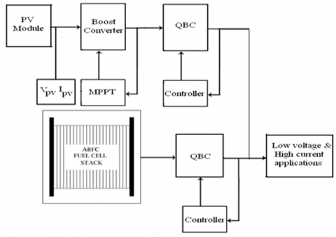
Figure 2 shows the proposed schematic of the ABFC power system. The following sections give the design and modelling of each block. The simulation results are presented at each stage to demonstrate the functionality of the models.
Figure 2. Proposed ABFC and PV module power system
2.1 ABFC stack model
At standard state conditions of 25°C and 1 atm (101.25 kPa), the standard potential from a hydrogen/oxygen fuel cell is around 1.229V. However, the cell potential drops from equilibrium value due to irreversible losses. The different irreversible losses are activation, ohmic, and concentration losses. The ABFC output voltage [7-9] is given by Eqns. (4) - (10).
$\mathrm{V}_{\text {Fuelcell }}=\mathrm{V}_{\text {Opencircuit }}-\Delta \mathrm{V}_{\text {Activation }}$ $-\Delta \mathrm{V}_{\text {Ohmic }}-\Delta \mathrm{V}_{\text {Concentration }}$ (4)
$\mathrm{V}_{\text {Openciruuit }}=\mathrm{V}_{\text {Nemst }}-\mathrm{V}_{\text {Cross }}$ (5)
$V_{\text {poterialNernst }}=1.482-0.000845^{*} T$
$+0.0000431^{*} T^{*} \ln \left(\rho_{\mathrm{H}_{2}} * \rho_{\mathrm{O}_{2}}^{0.5}\right)$ (6)
$V_{\text {Cross }}=\frac{R T}{\alpha F} \ln \left(\frac{i_{\text {Cross }}}{i_{0}}\right)$ (7)
$\rho_{\mathrm{H}_{2}}=\frac{0.5 \mathrm{P}_{\mathrm{H}_{2}}}{\exp \left(\frac{1.653 * \mathrm{i}}{\mathrm{T}_{\mathrm{ADP}}^{1.334}}\right)}-\mathrm{P}_{\mathrm{Sat}}$ (8)
$\rho_{\mathrm{O}_{2}}=\frac{\mathrm{P}_{\mathrm{O}_{2}}}{\exp \left(\frac{4.192 * \mathrm{i}}{\mathrm{T}_{\mathrm{GDP}}^{1.334}}\right)}-\mathrm{P}_{\mathrm{Sat}}$ (9)
$\mathrm{P}_{\mathrm{Sat}}=10^{\left(-2.1794+0.02953 * \mathrm{T}-9.1837 * 10^{-5} * \mathrm{T}^{2}+1.4454^{*} 10^{-7} * \mathrm{T}^{2}\right)}$ (10)
The activation loss is presented using Eq. (11).
$\Delta \mathrm{V}_{\text {Activation }}=\frac{\mathrm{RT}}{\alpha \mathrm{F}} \ln \left(\frac{\mathrm{i}}{\mathrm{i}_{0}}\right)$ (11)
The ABFC activation losses are given by:
$\Delta \mathrm{V}_{\text {Activation }}=\frac{\mathrm{RT}}{\alpha \mathrm{F}} \ln \left(\frac{\mathrm{i}+\mathrm{i}_{\mathrm{cr}}}{\mathrm{i}_{0}}\right)$ (12)
The ohmic losses are modelled by Eq. (13) and Eq. (18).
$\Delta \mathrm{V}_{\mathrm{Ohm}}=\mathrm{i} * \mathrm{r}_{\mathrm{Ohm}}$ (13)
$\begin{align} & {{r}_{Ohm}}={{r}_{resis\tan ceAnode}}+{{r}_{resis\tan ceCathode}} \\ & +{{r}_{resis\tan ceIonic}}+{{r}_{resis\tan ceContact}} \\ \end{align}$ (14)
$\mathbf{r}_{\text {resis tan ceAnode }}=\frac{\rho_{\mathrm{GDL} * \mathrm{L}_{\mathrm{GDL}}}}{\mathrm{A}_{\text {cellarea }}}+\frac{\rho_{\mathrm{Gr} * \mathrm{L}_{\mathrm{Gr}}}}{\mathrm{A}_{\text {cellarea }}}$ (15)
$\mathrm{r}_{\text {resis tan ceCathode }}=\frac{\rho_{\mathrm{GDL}^{*} \mathrm{L}}}{\mathrm{A}_{\text {cellarea }}}+\frac{\rho_{\mathrm{Gr}^{*} \mathrm{L}}}{\mathrm{A}_{\text {cellarea }}}$ (16)
$\mathrm{r}_{\mathrm{Ionic}}=\frac{\mathrm{L}_{\mathrm{Membrane}}}{\sigma \mathrm{A}_{\mathrm{C}}}$ (17)
$\sigma=(0.005169 * \lambda-0.00326) * \exp \left(1268\left(\frac{1}{303}-\frac{1}{\mathrm{T}}\right)\right)$ (18)
Eq. (19) presents the concentration losses given by:
$\Delta \mathrm{V}_{\text {ConcentrationLosses }}=\frac{\mathrm{RT}}{\mathrm{nF}}\left(1+\frac{1}{\alpha}\right) \ln \left(\frac{\mathrm{i}_{\mathrm{L}}}{\mathrm{i}_{\mathrm{L}}-\mathrm{i}}\right)$ (19)
2.2 Photovoltaic module
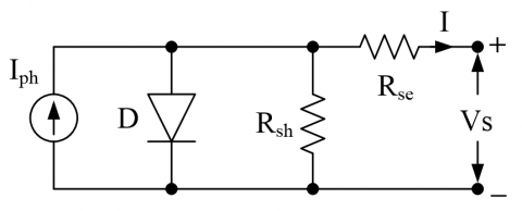
Figure 3 gives the solar cell [10] the equivalent circuit. The Iph, Rsh and Rse represent the cell photo current, shunt and series resistances respectively.
Figure 3. Equivalent circuit of PV cell
The photo current of PV module is given by Eq. (20).
$\mathrm{I}_{\text {photon }, \mathrm{PV}}=\left[\mathrm{I}_{\mathrm{scr}, \mathrm{PV}}+\mathrm{K}_{\mathrm{i}}(\mathrm{T}-298)\right] * \frac{\mathrm{G}}{1000}$ (20)
The reverse saturation current is shown by Eq. (21).
$\mathrm{I}_{\text {reversesaturation, } \mathrm{PV}}=$
$\mathrm{I}_{\mathrm{scr}, \mathrm{PV}} /\left[\exp \left(\mathrm{qv}_{\mathrm{oc}} / \mathrm{N}_{\mathrm{s}} \mathrm{KaT}\right)-1\right]$ (21)
The saturation current IO is given by Eq. (22).
$\mathrm{I}_{\text {saturation, } \mathrm{PV}}=\mathrm{I}_{\text {reversesaturation }, \mathrm{PV}}$
$\left[\frac{\mathrm{T}}{\mathrm{T}_{\mathrm{rs}}}\right]^{3} \exp \left[\frac{\mathrm{q}_{\mathrm{e}} * \mathrm{E}_{\mathrm{g}}}{\mathrm{aK}}\left\{\frac{1}{\mathrm{T}_{\mathrm{rs}}}-\frac{1}{\mathrm{T}}\right\}\right]$ (22)
The PV module current output is represented by Eq. (23).
$\mathrm{I}_{\mathrm{PV}}=\mathrm{N}_{\text {parallel }} * \mathrm{I}_{\mathrm{ph}, \mathrm{PV}}-\mathrm{N}_{\text {parallel }} * \mathrm{I}_{\text {saturation }}$
$\left[\exp \left\{\mathrm{q}_{\mathrm{e}}^{*}\left(\mathrm{V}_{\mathrm{PV}}+\mathrm{I}_{\mathrm{PV}} \mathrm{R}_{\mathrm{S}}\right) / \mathrm{N}_{\text {series }} \mathrm{aKT}\right\}-1\right]$ (23)
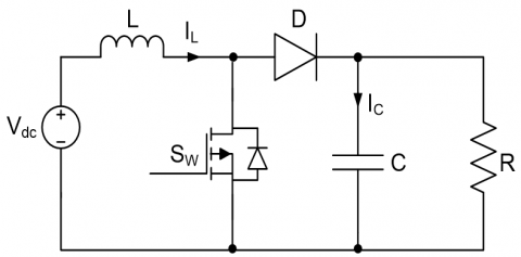
3.1 Boost converter with MPPT
Figure 4 highlights the schematic of the boost converter with its input-output voltage relation is given by Eq. (24).
$V_{0}=\frac{V_{S}}{(1-D)}$ (24)
Perturb & Observe (P&O) algorithm [10] is widely used MPPT technique for boost converter. P & O MPPT algorithm inscribes that for small perturbations in panel voltage, ∆P is positive, then the desired path is in the direction of MPP, hence the duty cycle (δ) has to be incremented and continue in the same way. If ∆P is negative, then the path deviates from MPP, hence the duty cycle (δ) has to be decremented. If ∆P is zero, it indicates MPP. The boost converter is prominent for MPPT.
Figure 4. Schematic of boost converter
3.2 QBC with ACMC
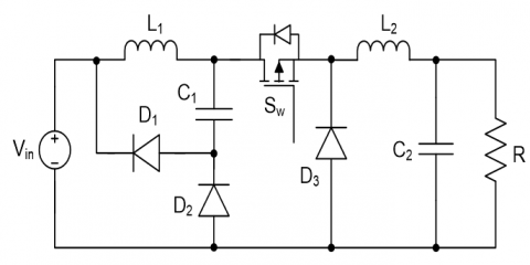
QBC is used as a PCU [11, 12] whose schematic is shown in Figure 5 along with its voltage conversion ratio represented by Eq. (25).
$\mathrm{M}(\mathrm{D})=\frac{\mathrm{V}_{\mathrm{o}}}{\mathrm{V}_{\mathrm{in}}}=\mathrm{D}^{2}$ (25)
Figure 5. Quadratic buck converter
4.1 ABFC and PV module
The literature [7-9] gives the simulation parameters of an ABFC shown in Table 1. As represented in Figure 2 for ABFC power system, the output of ABFC stack goes to the QBC. Table 2 highlights the electrical characteristics of a 30 W PV module. In the solar PV power system, the PV module output is fed to the boost converter for MPPT. The boost converter output is given as input to the QBC. The simulation parameters of continuous conduction mode (CCM) based QBC and boost converter are tabulated in Table 3. In both converters, the CCM operation results in low losses and high efficiency.
Table 1. ABFC simulation parameters
|
Parameter |
Value |
|
GDL ρ |
0.0017 Ω-Cm |
|
GDL ρ |
0.036 Cm |
|
Graphite ρ |
0.00231 Ω-Cm |
|
Graphite Flow Channel Thickness |
0.1 Cm |
|
Membrane Thickness |
0.0178 Cm |
|
λ |
12 |
|
icr |
3 mA/Cm2 |
|
Contact resistance (r) |
30 Ω-Cm2 |
Table 2. Electrical characteristics of 30 W PV module
|
Simulation parameter |
Value |
|
Prated |
30W |
|
Vmp |
19V |
|
Voc |
27.5V |
|
Isc |
1.83A |
|
Ns |
47 |
|
Np |
1 |
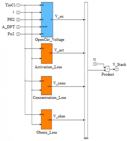
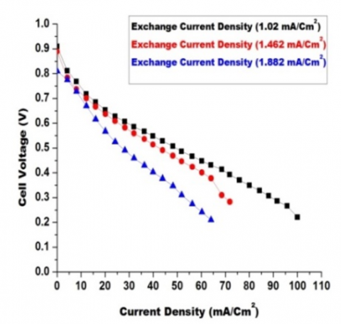
Figure 6 shows the MATLAB ABFC stack model based on Eqns. (4)-(19). This model includes the activation loss, ohmic loss, mass transportation and Nernst open circuit voltage blocks for realizing the actual behaviour of the ABFC. The Polarisation characteristic of the single ABFC is shown in Figure 7. The cell voltage curves for various exchange current densities are shown in Figure 8.
As shown in Figure 7, with increasing current densities the ABFC voltage falls and concomitantly degrades the efficiency. Whereas, the power density at first increases to a maximum value and thereafter decreases with respect to the current density. Hence, there should be a trade-off between the power density and efficiency. This is very critical while designing the portable and stationary applications. In Figure 8, the voltage curves are shown for different exchange current densities which depend on the temperature. It means that, at higher temperatures the ABFC voltage drops.
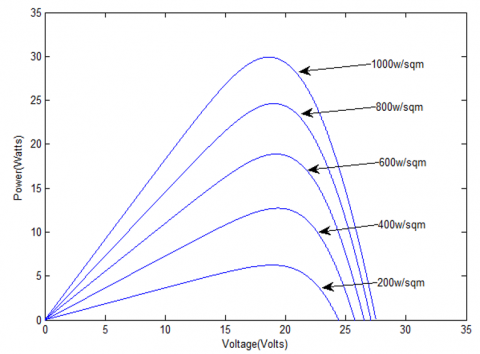
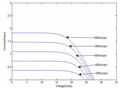
Figure 9 and Figure 10 show the P-V and I-V characteristics at 25℃ with different irradiation levels. Figure 11 shows the MPP tracking at t=4sec for 300 w/sq.m to 600 w/sq.m irradiation change and also 600 w/sq.m to 1000 w/sq.m irradiation change at t=6sec. The P&O MPPT algorithm is effective for tracking the rated power of 30 W. It is also observed that, the tracking speed of MPP is good with this algorithm.
Table 3. QBC specifications
|
Fuel cell stack |
|
|
Voltage |
19V |
|
Current |
1.579A |
|
Power rating |
30W |
|
Boost converter |
|
|
Vin |
18 ~ 27 V |
|
L |
100 µH |
|
C |
0.2 µF |
|
fsw |
50 kHz |
|
VO |
35 V |
|
Quadratic buck converter |
|
|
Parameter |
Nominal value |
|
Vin |
19 ~ 35 V |
|
L1 |
1.84 µH |
|
L2 |
0.21 µH |
|
C1 |
22 µF |
|
C2 |
1.64 mF |
|
Schottky FVD forwarvoltage drop |
0.30 V |
|
fsw |
300 kHz |
|
Load Rmin |
0.0333 Ω |
|
Load Rmax |
0.2 Ω |
|
Output voltage |
1 V |
|
Output power |
30 W |
Figure 6. MATLAB model of ABFC
Figure 7. ABFC polarisation characteristic
Figure 8. ABFC cell voltage curve at various exchange current densities
Figure 9. P-V characteristics
Figure 10. I-V characteristics
Figure 11. MPP tracking for three different irradiations using P&O MPPT algorithm
4.2 Power conditioning unit
4.2.1 Controller performance at a stack voltage of 18.665V with step load change
The transfer functions (TF) of filter in current loop, current loop compensator and voltage loop compensator are given in Eq. (26), Eq. (27) and Eq. (28).
The current feedback loop low pass filter TF is obtained as:
$\mathrm{F}(\mathrm{s})=\frac{12600}{(\mathrm{s}+12600)}$ (26)
The PI controller TF in current loop is obtained as
$C_{1}(s)=\frac{100(1+0.02 s)}{s}$ (27)
The PI controller TF in voltage loop is obtained as
$C_{2}(s)=\frac{20(1+0.1 s)}{s}$ (28)
The compensator design is fulfilled in MATLAB/siso tool. The corner frequency of low pass filter is equal to 300 kHz. The crossover frequency of current loop (bandwidth) is greater than the voltage loop. The current and voltage loops have gain margin (GM) and phase margin (PM) of 6.32dB, 46.7° & 23.7dB, 48.7° ensuring a stable system.
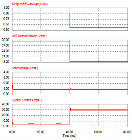
As shown in Figure 12, ABFC stack voltage is given as input to QBC and at 40 m sec for 5A -30A step load. The observed transient voltage deviation is 28% with a settling time of 0.75 msec. Moreover, each fuel cell undergoes a voltage reduction from 0.889 V to 0.565 V, the fuel cell stack voltage reduces from 29.337 V to 18.645 V.
4.2.2 Controller performance for periodic load change at a fuel cell stack voltage of 18.665V
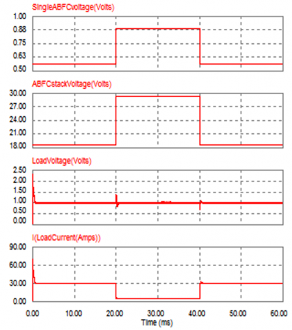
As shown in Figure 13, during load decrease (30A-5A) the transient output voltage rise is 25% with a settling time of 1.5 msec, and 28% voltage dip during step load increase (5A-30A) having a settling time of 0.75 msec. Moreover, ABFC voltage increases from 0.565 V to 0.889 V and vice-versa, the fuel cell stack voltage increases from 18.645 V to 29.337 V and vice-versa.
Figure 12. QBC input and output waveforms
Figure 13. QBC input and output waveforms
During step increase in load from 5A-30A, the ABFC stack voltage decreases from 29.337 V to 18.645 V due to more voltage drop across the ohmic resistance (Rohmic) and vice-versa.
4.3 Efficiency analysis of QBC
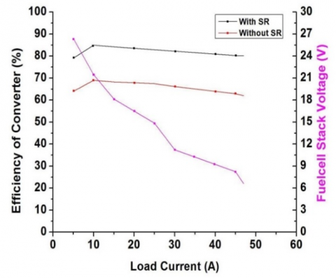
Normally, the power diodes exhibit more forward voltage drop (FVD) of around 1V. Therefore, their usage can degrade the QBC efficiency due to more conduction losses. This problem can be overcome by using schottky diodes of low FVD (around 0.3V) in place of power diodes. But still the obtained efficiencies are not up to the mark in case of low voltage and high current applications. The other viable solution is the adoption of Synchronous Rectification (SR). As shown in Figure 5, the schottky diode D3 is replaced by a power MOSFET having very low on-state resistance (Ron) in order to achieve a remarkable QBC efficiency [12]. Figure 14 shows the efficiency comparison of QBC without and with SR, also fuel cell stack voltage for different load currents.
Figure 14. The efficiency of QBC and fuel cell stack voltage
At rated input voltage of 19 V, without SR, the efficiency is found to be 65.20%. With SR, the lower power MOSFET incorporated in place of D3 has a very low Ron of 1.88 mΩ and the efficiency is found to be 81.90%. The SR enhances the converter efficiency by 16.70%.
4.4 Efficiency of ABFC and PV Cell
The ABFC theoretical efficiency of 83.0% is obtained by:
$\eta_{\mathrm{FC}}=\frac{\mathrm{V}_{\mathrm{Cell}}}{1.482}$ (29)
With SR the theoretical ηmax is 67.97%, and without SR the η is 54.116%. The efficiencies of buck and boost converter are found to be 91.4% and 91.9%, the PV cell theoretical η is 30.0%. At rated load, PV module power system theoretical η with SR is found to be 25.116%.
In this paper the modelling of Air Breathing Fuel Cell (ABFC) and solar PV based power system is presented. In ABFC power system the QBC is implemented with ACM control strategy and the simulation results associated with step load as well as periodic load are highlighted. For step load change, ABFC as well as stack voltage decreases to 0.33 V and 10.68 V. At rated load without and with SR, the theoretical ηmax of ABFC power system are 54.116% and 67.97%. The SR enhances ABFC system η by 13.854%. In PV module power system at 25°C with different irradiation levels the boost converter effectively tracks the maximum power. At rated load, the overall PV module PS η is found to be 25.116%. Even though low efficiencies are obtained in case of ABFC as well as solar panel, the important aspect is that they are the inexhaustible sources of energy.
|
V |
Voltage, V |
|
A |
Active area of cell, cm2 |
|
ΔV |
Overpotential, V |
|
R |
Gaseous constant, J/mol K |
|
F |
Faraday’s constant, C/mol |
|
p |
Partial pressure of hydrogen, bar |
|
P |
Pressure of hydrogen, bar |
|
PSat |
Saturation pressure of water, bar |
|
i |
Current density, mA/cm2 |
|
icr |
Crossover current, mA/cm2 |
|
iL |
Limiting current density, mA/cm2 |
|
io |
Exchange current density, mA/cm2 |
|
r |
Ohmic resistance, Ω-cm2 |
|
LM |
Thickness of membrane, cm |
|
T |
Temperature, K |
|
K |
Boltzmann’s constant, J/K |
|
I |
Current, A |
|
q |
Charge of electrons, C |
|
a |
Ideality factor |
|
Eg |
Energy gap, eV |
|
N |
Number of cells |
|
G |
Solar irradiation, W/m2 |
|
Prated |
Rated power |
|
Ki |
Short-circuit current temperature coefficient |
|
D |
Duty cycle |
|
C |
Capacitor, F |
|
L |
Inductor, H |
|
fsw |
Switching frequency, Hz |
|
Greek letters |
|
|
α |
Charge transfer coefficient |
|
λ |
Water drag coefficient |
|
σ |
Conductivity of membrane, S/cm |
|
ρ |
Specific resistance, Ω-cm |
[1] Souleman, N.M., Olivier, T., Louis, A.D. (2012). Development of a generic fuel cell model: application to a fuel cell vehicle simulation. International Journal of Power Electronics, 4(6): 505-522. https://doi.org/10.1504/IJPELEC.2012.052427
[2] Kumar, M.P., Kumar, A.K. (2010). Effect of cathode channel dimensions on the performance of an air-breathing PEM fuel cell. International Journal of Thermal Sciences, 49(5): 844-857. https://doi.org/10.1016/j.ijthermalsci.2009.12.002
[3] Jia, J., Li, Q., Wang, Y., Cham, Y.T., Han, M. (2009). Modeling and dynamic characteristic simulation of proton exchange membrane fuel cell. IEEE Trans. Control Syst. Technol., 24(16): 283-291. https://doi.org/10.1109/TEC.2008.2011837
[4] Standford, E. (2003). Power technology roadmap for microprocessor voltage regulators. In: Proc. PSMA, Feb. 2003.
[5] Xie, X.G., Qian, Z.M. (2008). A new two-stage buck converter for voltage regulators. Power Electronics Specialists Conference (PESC), Rhodes, Greece, pp. 1580-1584. https://doi.org/10.1109/PESC.2008.4592164
[6] Ajayan, S., Selvakumar, I.A. (2020). Modeling and simulation of PEM fuel cell electric vehicle with multiple power sources. International Journal of Recent Technology and Engineering, 8(6): 2967-2975. https://doi.org/10.35940/ijrte.F8420.038620
[7] Amphlett, J.C., Baumertr, M., Mannr, F. (1995). Performance modeling of the Ballard mark IV solid polymer electrolyte fuel cell: Empirical model development. Journal of The Electrochemical Society, 142(1): 9-15. https://doi.org/10.1149/1.2043959
[8] Kim, J., Lees, M., Srinivasan, S. (1995). Modelling of proton exchange membrane fuel cell performance with an empirical equation. Journal of the Electrochemical Society, 142(8): 2670-2674. https://doi.org/10.1149/1.2050072
[9] Tagore, R.Y., Anuradha, K., Babu, V.A.R., Kumar, M.P. (2019). Modelling, simulation and control of fuel cell powered laptop computer voltage regulator module. International Journal of Hydrogen Energy, 44(21): 11012-11019. https://doi.org/10.1016/j.ijhydene.2019.02.141
[10] Ganesh, G., Kumar, V.G., Babu, V.A.R., Rao, S.G., Tagore, R.Y. (2015). Performance analysis and MPPT control of a standalone hybrid power generation system. Journal of Electrical Engineering, 15(1): 334-343.
[11] Yadlapalli, R.T., Narasipuram, R.P., Kotapati, A. (2020). An overview of energy efficient solid state LED driver topologies. International Journal of Energy Research, 44(2): 612-630. https://doi.org/10.1002/er.4924
[12] Yadlapalli, R.T., Kotapati, A. (2014). A fast-response sliding-mode controller for quadratic buck converter. International Journal of Power Electronics (IJPELEC), 6(2): 103-130. https://doi.org/10.1504/IJPELEC.2014.061468