Ahmed Bennaoui* | Slami Saadi | Aissa Ameur
© 2020 IIETA. This article is published by IIETA and is licensed under the CC BY 4.0 license (http://creativecommons.org/licenses/by/4.0/).
OPEN ACCESS
Some studies tried to make transition from Type-1 to interval Type-2 membership functions, but they get the problems of choosing the footprint uncertainty size in the Interval Type-2 Membership Functions. In this paper, our objective is to employ two optimization methods: Invasive Weed Optimization (IWO) and Particle Swarm Optimization (PSO) for tuning the Transitioning from Type-1 To Interval Type-2 Fuzzy Logic Controller for Boost DC-DC Converters and compare their performances. Also, we will discuss the effects of the PID values in the operation of transition from Type-1 to interval Type-2 fuzzy logic Controller for Boost DC-DC Converters. The simulation results show IWO optimization methods is helpful to Tuning the Transitioning from Type-1 To Interval Type-2 Fuzzy Logic Controller for Boost DC-DC Converters. Moreover, when we tune both PID values and the FOU size in T2-MFs of Interval Type-2 Fuzzy Logic PID-controller, we will get the best performance for interval Type-2 Fuzzy Logic PID-controller for Boost DC-DC Converter. To sum up; the optimal footprint of uncertainty (FOU) size in interval Type-2 membership functions, they have an essential role and good effect in the performance of Interval Type-2 fuzzy logic Controller for Boost DC-DC Converters.
IWO, Type-2 fuzzy logic controller, Type-1 membership functions, interval Type-2 membership functions, footprint of uncertainty (FOU)
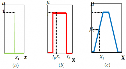
The membership functions (MFs) enable establishing a relationship between numerical values and linguistic labels.
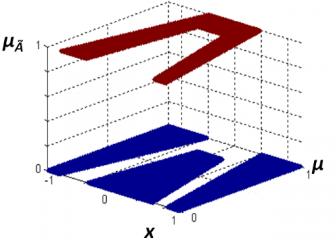
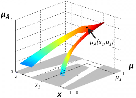
Type-1 fuzzy MFs (T1-MF) are two dimensional and represent the membership degree μ for a variable x. Type-2 fuzzy MFs (T2-MF) are three dimensional:
They consider an uncertainty U of the membership degree. T1-MFs are a particular case of T2-MFs where the uncertainty value is 0. Membership functions are classified as (Figure 1 and Figure 2):
The concept of Type-2 fuzzy set was initially proposed as an extension ofType-1 fuzzy set by Prof. Zadeh [1].
Figure 1. Membership functions (a) singleton, (b) Interval Type-1, (c) Type-1
(a)
(b)
Figure 2. Membership functions (a) interval Type-2, (b) general Type-2
The Type-2 fuzzy system is characterized by a fuzzy membership function, i.e., the membership grade for each element of this set is a fuzzy set in [0,1], contrary a Type-1 fuzzy set where the membership grade is a crisp number in [0,1]. Such sets are very useful in circumstances where they are difficult to determine an exact membership function for a fuzzy set; hence, they are useful for incorporating uncertainties. Type-2 fuzzy sets are appropriate for modeling uncertainty as Type-2 fuzzy sets include FOU (Footprint of Uncertainty) and third dimension, offering extra degrees of freedom to Type-2 fuzzy sets in comparison to Type-1 fuzzy sets [2, 3].
The performance of Type-2 Fuzzy Logic Controller (T1 FLC) is affected by the Footprint of uncertainty size in interval Type-2 membership functions [4-8].
Some studies propose [7, 8] to transition from type-l to interval Type-2 fuzzy sets, through varying the size FOU (Footprint of uncertainty) in interval Type-2 membership functions, but there are problems of tuning the footprint of uncertainty size parameter in The Interval Type-2 Membership Functions.
In this work, we developed a new approach to transit from Type-1 to interval Type-2 fuzzy logic Controller using the optimization methods (IWO and PSO). Also, we used the optimization methods (IWO and PSO) for tuning the PID values and the footprint uncertainty size in the Interval Type-2 Membership Functions of Interval Type-2 Fuzzy Logic PID Controller for Boost DC-DC Converters.
This paper will be organized as following:
Section 2: Converter modeling. section 3: The Type-2 TSK Fuzzy Logic Controller. section 4: Invasive Weed Optimization Algorithm. section 5: Fuzzy PID Controller for Boost DC-DC Converters. section 6: Simulation Phases and Results. section 7: Conclusion.
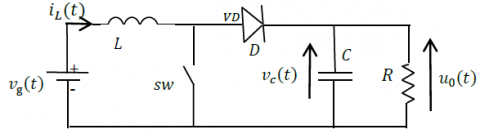
In this study we will use the DC–DC Boost converter (Figure 3 and Table 1).
Figure 3. The DC–DC boost converter
Table 1. The parameters of the DC–DC boost converter
|
the parameters of |
the DC–DC Boost converter |
|
Series Inductance |
$\mathrm{L}=20[\mathrm{mH}]$. |
|
Parallel Capacitance |
$\mathrm{C}=20[\mu \mathrm{f}]$ |
|
load resistance |
$\mathrm{R}=30[\Omega]$ |
|
Input Voltage |
$\mathrm{Vg}=15[\mathrm{V}]$ |
|
Switching frequency |
$\mathrm{f}_{\mathrm{SW}}=5[\mathrm{kHz}]$. |
Vg: Represents power supply voltage. iL: The current through the inductance L. sw: An electronic switch. VD: Voltage of the diode. Vc: The voltage on the capacitor C. u0(t) Voltage output across the resistive load R.
Continuous conduction mode (CCM) has two topologies depending on the position of switch swand. In this simulation, we use the Boost DC-DC Converter operating in continuous conduction mode (CCM).
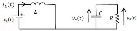
The following equations represent the first topology (Figure 4) of DC–DC Boost converter:
$L \frac{d}{d t} \mathrm{i}_{L}(t)=V_{\mathrm{g}}(t)$
$\frac{d}{d t} v_{\mathrm{c}}(t)=-\frac{1}{C R} v_{c}(t)$ (1)
$u_{0}(t)=v_{c}(t)$
Figure 4. The first topology (sw closed, VD opened)
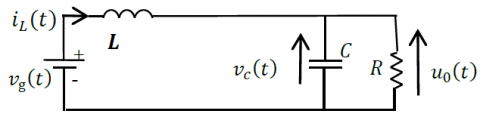
The following equations represent the second topology (Figure 5) of DC–DC Boost converter:
Figure 5. The second topology (sw opened, VD closed)
$L \frac{d}{d t} \mathrm{i}_{L}(t)=v_{\mathrm{g}}(t)-v_{c}(t)$
$\frac{d}{d t} v_{c}(t)=\frac{1}{C R}\left(R \mathrm{i}_{L}(t)-v_{\mathrm{c}}(t)\right)$ (2)
$u_{0}(t)=v_{c}(t)$
The state equation of the boost DC-DC converter can be stated as [9]:
$\dot{x}=A_{i} x+B_{i} V_{\mathrm{g}}(t)$
$u_{0}=C_{i} x$ with $x=\left[i_{L} v_{\mathrm{c}}\right]^{T}$ (3)
where, subscript 1 stands for transistor ON, and subscript 2 stands for transistor OFF of the converter circuit.
$A_{i}, B_{i}$ and $C_{i}$ are system Matrices of the constituent linear circuits.
The system matrices can be obtained for different operating modes as:
$C_{1}=[0 \quad 1], C_{2}=[0 \quad 1] \cdot A_{1}=\left[\begin{array}{cc}0 & 0 \\ 0 & -\frac{1}{R C}\end{array}\right],$ and $A_{2}=$$\left[\begin{array}{cc}0 & -\frac{1}{L} \\ \frac{1}{c} & -\frac{1}{R C}\end{array}\right] \cdot B_{1}=B_{2}=\left[\frac{1}{L} 0\right]^{T}$
The State-Space Averaged model represented in the following equations [10-13]:
$\left\{\begin{array}{c}\dot{x}=A_{a v g} x+B_{a v g} u \\ a n d \\ y=C_{a v g} x\end{array}\right.$ (4)
where, $\left\{\begin{array}{l}A_{a v g}=d A_{1}+(1-d) A_{2} \\ B_{a v g}=d B_{1}+(1-d) B_{2} \\ C_{a v g}=d C_{1}+(1-d) C_{2}\end{array}\right.$
A Type-2 TSK fuzzy logic controller was firstly introduced by Mendel and Liang. We have three models of T2 TSK fuzzy logics based on the type of the antecedent and consequent part of rules [14-16] (Table 2 and Table 3).
Table 2. Classification of other t2 tsk fls models [15, 16]
|
|
Antecedent |
Consequent |
The Rule Base |
|
T2 TSK FLS Model I |
Type-2 fuzzy sets |
Type-1 fuzzy sets |
IF $\mathrm{x}_{1}$ is $\tilde{\mathrm{F}}_{1}^{\mathrm{i}}$ and... $\mathrm{x}_{\mathrm{p}}$ is $\tilde{\mathrm{F}}_{\mathrm{p}}^{\mathrm{i}}$ THEN $\mathrm{y}^{1}=\mathrm{C}_{0}^{1}+\mathrm{C}_{1}^{1} \mathrm{x}_{1} \ldots+\mathrm{C}_{\mathrm{p}}^{1} \mathrm{x}_{\mathrm{p}}$ |
|
T2 TSK FLS Model II |
Type-2 fuzzy sets |
Crisp Numbers |
IF $\mathrm{x}_{1}$ is $\tilde{\mathrm{F}}_{1}^{\mathrm{i}}$ and... $\mathrm{x}_{\mathrm{p}}$ is $\tilde{\mathrm{F}}_{\mathrm{p}}^{\mathrm{i}}$ THEN $\mathrm{y}^{1}=\mathrm{C}_{0}^{1}+\mathrm{C}_{1}^{1} \mathrm{x}_{1} \ldots+\mathrm{C}_{\mathrm{p}}^{1} \mathrm{x}_{\mathrm{p}}$ |
|
T2 TSK FLS Model III |
Type-2 fuzzy sets |
Type-1 fuzzy sets |
IF $\mathrm{x}_{1}$ is $\tilde{\mathrm{F}}_{1}^{\mathrm{i}}$ and... $\mathrm{x}_{\mathrm{p}}$ is $\tilde{\mathrm{F}}_{\mathrm{p}}^{\mathrm{i}}$ THEN $\mathrm{y}^{1}=\mathrm{C}_{0}^{1}+\mathrm{C}_{1}^{1} \mathrm{x}_{1} \ldots+\mathrm{C}_{\mathrm{p}}^{1} \mathrm{x}_{\mathrm{p}}$ |
Table 3. The final output of other T2 TSK FLS models
|
|
The final output Of T2 TSK Models |
|
T2 TSK FLS- Model I |
The final output is also an interval Type-1 set and is calculated as follows [15-17]: $Y\left(Y^{1}, \ldots Y^{M}, F^{1}, \ldots, F^{M}\right)=\left[y_{l}, y_{r}\right]=\int_{y^{1}} \ldots \int_{y^{M}} \int_{f^{1}} \ldots \int_{f^{M}} 1 / \frac{\sum_{i=1}^{M} f^{i} y^{i}}{\sum_{i=1}^{M} f^{i}}$ Where M is the number of rules fired, $y_{i} \in Y^{i},$ and $Y^{i}=\left[ y_{1}^{i}, y_{r}^{i}\right],(i=1 \ldots M)$ |
|
T2 TSK FLS -Model II |
The final output Is a special case of (5), because now each $Y^{i}$ is a crisp value $y^{i}$. So $Y\left(f^{1}, \ldots, f^{M}\right)=\left[y_{l}, y_{r}\right]=\int_{f^{1}} \ldots \int_{f^{M}} 1 / \frac{\sum_{i=1}^{M} f^{i} y^{i}}{\sum_{i=1}^{M} f^{i}}$ |
|
T2 TSK FLS -Model III |
The final output is special case of (5), because now each $F^{i}$ is a crisp value $f^{i}$ So $Y\left(Y^{1}, \ldots Y^{M}\right)=\left[y_{l}, y_{r}\right]=\int_{y^{1}} \ldots \int_{y^{M}} 1 / \frac{\sum_{i=1}^{M} f^{i} y^{i}}{\sum_{i=1}^{M} f^{i}}$ |
where, $i=1,2, \ldots \ldots \ldots, M, C_{k}^{i}(k=1,2, \ldots, p)$ are the consequent parameters whitch are Type-1 fuzzy set, $c_{k}^{i}(k=1,2, \ldots, p)$ are the consequent parameters that are crisp numbers, $Y^{l}$ are the outputs of the $l^{\text {th }}$ rule, $\tilde{F}_{j}^{i}(j=1 \ldots . . p \text { ) are Type- } 2$ fuzzy sets of input state $j$ in rule $M,$ given an inputs $x_{1}, x_{2} \ldots \ldots x_{p}, F_{j}^{i}(j=1 \ldots \ldots p)$ are Type- 1 fuzzy sets.
The firing strength of the ith rule $F^{i}(x)$ with meet operation under product or minimum t-norm is an interval Type-1 set expressed as:
$F^{i}(x)=\left[\underline{f}^{i}(x), \bar{f}^{i}(x)\right]$ (5)
where,
$\underline{f}^{i}(x)=\underline{\mu}_{\tilde{F}_{1}^{i}}\left(x_{1}\right) * \ldots \underline{\mu}_{\tilde{F}_{p}^{i}}\left(x_{p}\right)$
$\bar{f}^{i}(x)=\bar{\mu}_{\tilde{F}_{1}^{i}}\left(x_{1}\right) * \ldots \bar{\mu}_{\tilde{F}_{p}^{i}}\left(x_{p}\right)$
To compute Y it is only necessary to compute its two end-points y1 and yr can also be computed more efficient by the KM Algorithm and the Defuzzified output is:
$y=\frac{y_{l}+y_{r}}{2}$ (6)
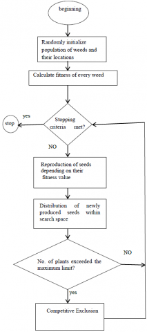
Invasive weed optimization (IWO) was developed by Mehrabian and Lucas in 2006 [18, 19], The invasive weed optimization technique is a population-based evolutionary optimization method inspired by the behavior of weed colonies, Invasive weed optimization technique has been successfully used to a variety of optimization problems [20-25]. The process is addressed in these steps (Figure 6):
Figure 6. Invasive weed optimization algorithm flowchart
The procedure starts off evolved with initializing a population. Its capacity that a populace of preliminary options is randomly generated over the problem space. Then contributors of the population produce seeds relying on their relative fitness in the population. In other words, the range of seeds for every member is starting with the value of $\mathrm{S}_{\min }$ for the worst member and increases linearly to $\mathrm{S}_{\max }$ for the first-rate member. For next step, these seeds are randomly scattered over the search area by way of generally distributed random numbers with mean equal to zero and an adaptive standard deviation [18, 19]. the standard deviation (SD) [18, 19] for every generation is in:
$\sigma_{\text {iter }}=\frac{\left(\text { iter }_{\text {max }}-\text { iter }\right)^{\mathrm{n}}}{\left(\text { iter }_{\text {max }}\right)^{\mathrm{n}}}\left(\sigma_{\text {init }}-\sigma_{\text {final }}\right)+\sigma_{\text {final }}$ (7)
n: is the nonlinear modulation index, $\sigma_{\text {iter }}$ is the standard deviation at the current iteration and iter $_{\max }$: is the maximum number of iterations. The produced seeds, accompanied through their parents are viewed as the practicable solutions for the subsequent generation. Finally step, a competitive exclusion is conducted in the algorithm, i.e., after a number of iterations the population reaches its maximum, and an elimination mechanism have to be employed. To this end, the seeds and their parents are ranked together and those with better fitness live on and end up reproductive [18, 19].
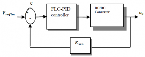
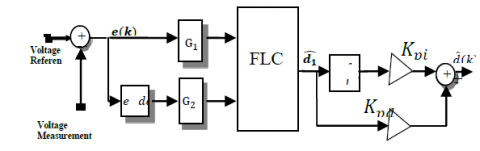
Fuzzy PID Controller systems (Figure 7 and Figure 8) have double inputs and single output. The error (e) and the change of error (de) are used as the inputs and the change of the control signal $\widehat{d_{1}}$ is used as the output of the FLC
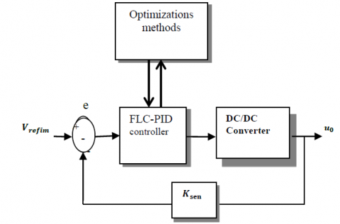
Figure 7. The FLC-PID controller for boost dc-dc converters
Figure 8. Structure of a fuzzy logic PID Controller (FLC-PID)
$K_{\mathrm{pi}}, K_{\mathrm{pd}}$ are values of PID.
$G_{1}, G_{2}$ values of the gains normalization of the fuzzy system inputs.
$\text { where, } G_{1}=0.5 \text { and } G_{2}=9$
The reference voltage: $\operatorname{Vref}=37.5 \mathrm{V}$. sensor of gain: $K_{\operatorname{sen}}$=0.04
And $V_{\text {refim }}=K_{\text {sen }} * V_{\text {ref }}, e=V_{\text {refim }}-K_{\text {sen }} * u_{0}$
This system is constructed from the human experience formulated in a collection of fuzzy rules in the following form:
$\mathrm{j}^{\mathrm{th}}: \mathrm{IF} \mathrm{e}$ is $\mathrm{E}_{0}^{\mathrm{j}}$ and $\operatorname{de}$ is $\mathrm{E}_{1}^{\mathrm{j}} \mathrm{THEN} $ $\hat{\mathrm{d}}_{1}=\mathrm{C}_{\mathrm{j}}(\mathrm{e}, \mathrm{de})$
With $\mathrm{E}_{0}^{\mathrm{j}} \mathrm{E}_{1}^{\mathrm{j}}$ are respectively the fuzzy sets of the error voltage e and its time derivative de $C_{\mathrm{j}}$ is the $\mathrm{j}^{\text {th }}$ output singleton.
The strategy of fuzzy control is derived using the following knowledge on the system:
The change of duty cycle $\hat{\mathrm{d}}{1}$ must be large, when $u_{0}$ is far from the reference.
Vreffor provides a small response time.
The small change of duty cycle $\hat{\mathrm{d}}{1}$ is sufficient to reach the reference providing that $u_{0}$ approaches the reference.
The duty cycle must be unchanged as long as $u_{0}$ is in the vicinity of the reference with a sufficient approaching speed, for preventing the output overshoot.
When $u_{0}$ reaches the reference and continue growing up: first, we decrease the duty cycle change, then if $u_{0}$ remains closer to the reference, the duty cycle changes must be zero otherwise, it must be negative.
Thus, the final control action $\hat{\mathrm{d}}$ applied to the converter is given by:
$\hat{\mathrm{d}}=\mathrm{G}_{1} \hat{\mathrm{d}}_{1}+\mathrm{G}_{2} \int \widehat{\mathrm{d}}_{1} \mathrm{d}$ (8)
We obtain 25 fuzzy rules with 17 output singletons issued from the human expertise (Table 4).
Table 4. Rules and output membership functions [8, 26]
|
e\de |
PH |
PL |
Z |
NL |
NH |
|
PH |
1 |
0.81 |
0.49 |
0.36 |
0.25 |
|
PL |
0.64 |
0.36 |
0.16 |
0.04 |
0 |
|
Z |
0.16 |
0.04 |
0 |
-0.04 |
-0.16 |
|
NL |
0 |
-0.04 |
-0.16 |
-0.36 |
-0.64 |
|
NH |
-0.25 |
-0.36 |
-0.49 |
-0.81 |
-1 |
In this work, we propose using the optimizations methods (IWO and PSO) to tuning the footprint of uncertainty size (FOU) in interval Type-2 fuzzy sets. Besides; We discuss the effects of the PID values in the operation of transition from Type-1 to interval Type-2 fuzzy logic Controller for Boost DC-DC Converters (Figure 9).
Figure 9. The FLC-PID controller with optimizations methods
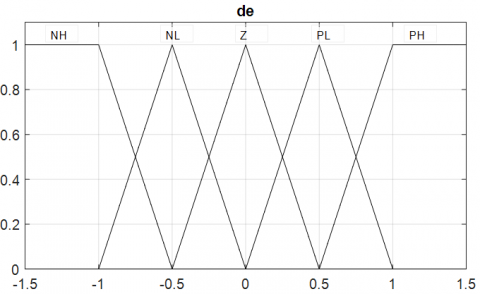
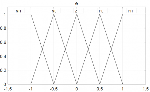
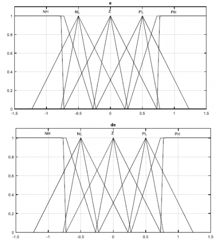
We use the two inputs fuzzy sets (e and de) are composed of five membership functions [8, 26] are defined in (Figure 10).
Figure 10. The two inputs fuzzy sets (e and de)
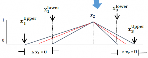
The transition from Type-1 membership functions to interval Type-2 membership functions shown in (Figure 11). [7, 8, 27]. The uncertainty size parameter (U) in the interval Type-2 membership functions is to be determined and optimized, using optimization algorithms (IWO and PSO).
Figure 11. Interval Type-2 membership functions [7, 8, 26]
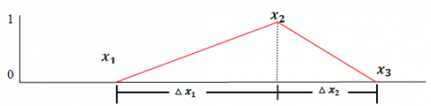
After make transition from Type-1membership functions (Figure 12) to interval Type-2 membership functions
Figure 12. Type-1 membership functions
where,
$\Delta \mathbf{x}_{1}=\mathbf{x}_{2}-\mathbf{x}_{1} ; \Delta \mathbf{x}_{2}=\mathbf{x}_{3}-\mathbf{x}_{2}$
The uncertainty (U) in the membership functions is the third considered parameter. we need to avoid overlapping between: $\mathrm{x}_{1}^{\text {lower }}$ and $\mathrm{x}_{3}^{\text {lower }},$ so, we propose: $\mathrm{U} \in[\mathbf{0}, \mathbf{1}] \Rightarrow \Delta \mathbf{x}_{1} * \mathbf{U} \leq$$\Delta \mathbf{x}_{1}$ and $\Delta \mathbf{x}_{2} * \mathbf{U} \leq \Delta \mathbf{x}_{2}$
$x_{1}^{\text {Upper }}=\max \left(-1, x_{1}-\Delta x_{1} * \mathbf{U} / 2\right)$.
$x_{1}^{l o w e r}=\max \left(-1+\Delta x_{1} * \mathbf{U}, x_{1}+\Delta x_{1} * \mathbf{U} / 2\right)$.
$x_{3}^{\text {lower }}=\min \left(1-\Delta x_{2} * \mathbf{U}, x_{3}-\Delta x_{2} * \mathbf{U} / 2\right)$.
$x_{3}^{\text {Upper }}=\min \left(x_{3}+\Delta x_{2} * \mathbf{U} / 2,1\right)$.
The uncertainty size Parameter (U) is to be determined and optimized, using optimization algorithms (IWO and PSO).
The objective function as following:
$\operatorname{cost}$ function $=\frac{\left(10^{3}\right)}{n} \sum_{t=0}^{n}[e(t)]^{2}$ (9)
In this work we have two types of simulation.
Firstly: tuning the FOU size in T2-MFsof Interval Type-2 Fuzzy Logic PID controller.
where,
Secondly: tuning both the PID values and the FOU size in T2-MFsof Interval Type-2 Fuzzy Logic PID controller.
where,
where, $\mathrm{K}_{\mathrm{pd}} \in[0,0.59]$ And $\mathrm{K}_{\mathrm{pi}} \in[0,450][26]$
In this paper, we developed a new approach to transit from Type-1 to interval Type-2 fuzzy logic Controller using the optimization methods (IWO and PSO). We have two types of simulation.
Table 5. The optimal controllers’ parameters
|
|
Optimizing the FOU size parameter (U) |
|
IT2F-PID controller with WO |
0.8534 |
|
IT2F-PID controller with PSO |
0.8534 |
|
Fuzzy Logic PID Controller (T1F-PID) [26] |
0 |
Table 6. Compare results obtained by IWO and PSO
|
|
ISE |
IAE |
TR |
Best-cost function |
|
IT2F-PID controller with IWO |
0.1087 |
0.1503 |
0.0206 |
108.7 |
|
IT2F-PID controller with PSO |
0.1087 |
0.1503 |
0.0206 |
108.7 |
|
Fuzzy Logic PID Controller (T1F-PID) [26] |
0.1559 |
0.2250 |
0.0306 |
\ |
Table 7. The optimal controllers parameters
|
|
Kpd |
Kpi |
the FOU size parameter (U) |
|
IT2F-PID controller with IWO |
0.590 |
392.6647 |
0.8219 |
|
IT2F-PID controller with PSO |
0.590 |
382.7533 |
0.8182 |
|
Fuzzy Logic PID Controller (T1F-PID) [26] |
0.25 |
255 |
0 |
Table 8. Compare results obtained by IWO and PSO
|
|
ISE |
IAE |
TR |
Best-cost function |
|
IT2F-PID controller with IWO |
0.0958 |
0.1202 |
0.0148 |
95.7732 |
|
IT2F-PID controller with PSO |
0.0963 |
0.1234 |
0.0160 |
96.3237 |
|
Fuzzy Logic PID Controller (T1F-PID) [26] |
0.1559 |
0.2250 |
0.0306 |
\ |
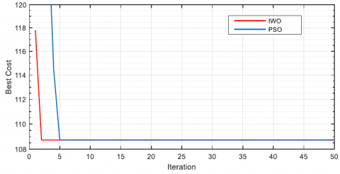
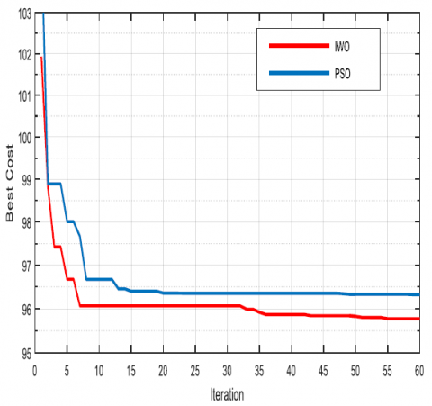
Figure 13. Iterative convergence curve
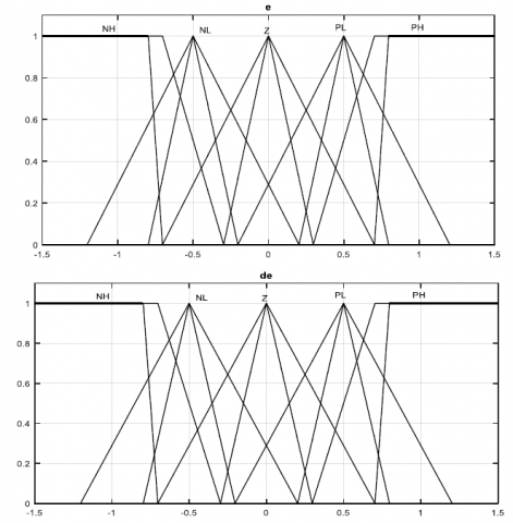
Figure 14. The Type-2 membership function of fuzzy sets of inputs interval Type-2 fuzzy logic controller after tuning by the IWO (the FOU size parameter U=0.8534)
Simulation results show:
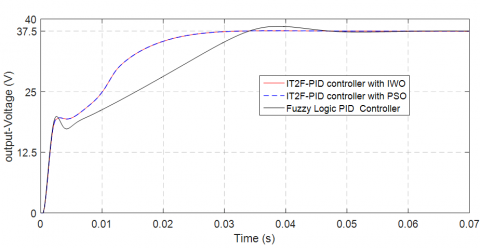
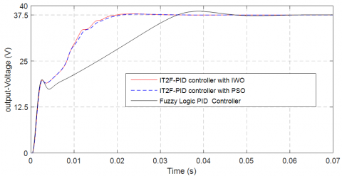
The Invasive weed optimization (IWO) algorithm converges quicker than the Particle Swarm Optimization algorithm (PSO) (Figure 13 and Figure 16). The superiority of the IT2F-PID controller with IWO comparing with both the IT2F-PID controller with PSO and fuzzy Logic PID controllers(Figure 15, Figure 18, Table 6 and Table 8), where: the IT2F-PID controller with IWO has minimum the Rise time (Tr), achieve lower the integral of square of errors (ISE) and the integral of the absolute errors (IAE) comparing with the other controllers. Finally; Invasive Weed Optimization Algorithm is helpful to tuning the PID values and the footprint of uncertainty size (FOU) in Interval Type-2 fuzzy logic PID controller for Boost DC-DC Converter.
Figure 15. The output voltage of different simulation cases
Figure 16. Iterative convergence curve
Figure 17. The Type-2 membership function of fuzzy sets of inputs Interval Type-2 fuzzy logic controller after tuning by the IWO (the FOU size parameter U=0.8219)
Figure 18. The output voltage of different simulation cases
[1] Zadeh, L.A. (1975). The concept of a linguistic variable and its application to approximate reasoning-I. Information Sciences, 8(3): 199-249. https://doi.org/10.1016/0020-0255(75)90036-5
[2] Mendel, J. (2017). Uncertain Rule-Based Fuzzy Systems Introduction and New Directions, 2nd Edition. Springer International Publishing AG 2017. https://doi.org/10.1007/978-3-319-51370-6
[3] Wu, D., Mendel, J.M. (2007). Uncertainty measures for interval Type-2 fuzzy sets. Information Sciences, 177(23): 5378-5393. https://doi.org/10.1016/j.ins.2007.07.012
[4] Zhou, H., Ying, H., Zhang, C. (2019). Effects of increasing the footprints of uncertainty on analytical structure of the classes of interval Type-2 Mamdani and TS fuzzy controllers. IEEE Transactions on Fuzzy Systems, 27(9). https://doi.org/10.1109/TFUZZ.2019.2892354
[5] Sepulveda, R., Melin, P., Rodriguez, A., Mancilla, A., Montiel. O. (2006). Analyzing the effects of the footprint of uncertainty in Type-2 fuzzy logic controllers. Engineering Letters, 13(2).
[6] Aladi, J.H., Wagner, C., Garibaldi, M.J., Pourabdollah, A. (2015). On transitioning from Type-1 to interval Type-2 fuzzy logic systems. IEEE International Conference on Fuzzy Systems (FUZZ-IEEE). https://doi.org/10.1109/FUZZ-IEEE.2015.7338004
[7] Martinez, J.S., Péra, M.C., Hissel, D. (2012). Type-2 fuzzy logic control of a DC/DC buck converter. Elsevier, IFAC Proceedings Volumes, 45(21): 103-108. https://doi.org/10.3182/20120902-4-FR-2032.00020
[8] Bennaoui, A., Saadi, S. (2017). Type-2 fuzzy logic PID controller and different uncertainties design for boost DC-DC converters. Springer, Electrical Engineering, 99(1): 203-211. https://doi.org/10.1007/s00202-016-0412-3
[9] Vidal-Ldiarte, E., Martine-Salamero, L., Guinjoan, F., Calvente, J., Gomariz, S. (2004). Sliding and fuzzy control of a boot converter using an 8-bit microcontroller. IEE Proceedings - Electric Power Applications, 151(1): 5-11. https://doi.org/10.1049/ip-epa:20040086
[10] Middlebrook, R.D., Cuk, S. (2006). Advances in Switched-Mode Power Conversion. Pasadena (California): TESLAco, cop.
[11] Vorperian, V. (1990). Simplified analysis of PWM converters using model of PWM switch part I and part II. IEEE Transactions on Aerospace and Electronic Systems, 26(3): 490-496. https://doi.org/10.1109/7.106126
[12] Lin, P.Z., Hsu, C.F., Lee, T.T. (2005). Type-2 fuzzy logic controller design for buck DC-DC converters. IEEE Xplore, The 14th IEEE International Conference on Fuzzy Systems, Reno, NV, USA. https://doi.org/10.1109/FUZZY.2005.1452421
[13] Krein, P.T., Bentsman, J., Bass, R.M., Lesieutre, B.L. (1990). On the use of averaging for the analysis of power electronic systems. IEEE Transactions on Power Electronics, 5(2): 182-190. https://doi.org/10.1109/63.53155
[14] Lynch, C., Hagras, H., Callaghan, V. (2006). Using uncertainty bounds in the design of an embedded realtime Type-2 neuro-fuzzy speed controller for marine diesel engines. IEEE International Conference on Fuzzy Systems Sheraton Vancouver Wall Centre Hotel, Vancouver, BC, Canada, pp. 1446-1453. https://doi.org/10.1109/FUZZY.2006.1681899
[15] John, R., Hagras, H., Castillo, O. (2018). Type-2 fuzzy logic and systems. International Publishing AG. Studies in Fuzziness and Soft Computing, 362. https://doi.org/10.1007/978-3-319-72892-6
[16] Fan, Q.F., Wang, T., Chen, Y., Zhang, Z.F., (2018). Design and application of interval Type-2 tsk fuzzy logic system based on QPSO algorithm. International Journal of Fuzzy Systems, 20(3): 835–846. https://doi.org/10.1007/s40815-017-0357-3
[17] Boumella, N., Djouani, K., Boulemden, M. (2012). A robust interval Type-2 TSK Fuzzy Logic System design based on Chebyshev fitting. Int. J. Control Autom. Syst., 10(4): 727–736. https://doi.org/10.1007/s12555-012-0408-3
[18] Mehrabian, A.R., Lucas, C. (2006). A novel numerical optimization algorithm inspired from weed colonization. Ecological Informatics, 1(4): 355-366. https://doi.org/10.1016/j.ecoinf.2006.07.003
[19] Xing, B., Gao, W.J. (2014). Invasive Weed Optimization Algorithm. In: Innovative Computational Intelligence: A Rough Guide to 134 Clever Algorithms. Intelligent Systems Reference Library, vol 62. Springer, Cham.
[20] Nagaraju, T.V., Prasad, D.C., Murthy, N.G.K. (2019). Invasive Weed Optimization Algorithm for Prediction of Compression Index of Lime-Treated Expansive Clays. Springer, Singapore, Soft Computing for Problem Solving, pp. 317-324. https://doi.org/10.1007/978-981-15-0184-5_28
[21] Mandava, R.K., Vundavilli, P.R. (2018). Implementation of modified chaotic invasive weed optimization algorithm for optimizing the PID controller of the biped robot. Sādhanā, 43(66). https://doi.org/10.1007/s12046-018-0851-9
[22] Goli, A., Tirkolaee, E.B., Malmir, B., Bian, G.B., Sangaiah, A.K. (2019). A multi-objective invasive weed optimization algorithm for robust aggregate production planning under uncertain seasonal demand. Computing, 101: 499–529. https://doi.org/10.1007/s00607-018-00692-2
[23] Zhao, X.Q., Zhou, J.H. (2015). Improved kernel possibilistic fuzzy clustering algorithm based on invasive weed optimization. Journal of Shanghai Jiaotong University (Science), 20(2): 164-170. https://doi.org/10.1007/s12204-015-1605-z
[24] Mohanty, P.K., Parhi, D.R. (2014). A new efficient optimal path planner for mobile robot based on Invasive Weed Optimization algorithm. Front. Mech. Eng., 9: 317–330. https://doi.org/10.1007/s11465-014-0304-z
[25] Misaghi, M., Yaghoobi, M. (2019). Improved invasive weed optimization algorithm (IWO) based on chaos theory for optimal design of PID controller. Journal of Computational Design and Engineering, 6(3): 284-295. https://doi.org/10.1016/j.jcde.2019.01.001
[26] Guesmi, K., Essounbouli, N., Hamzaoui, A. (2008). Systematic design approach of fuzzy PID stabilizer for DC–DC converters. Elsevier, Energy Conversion and Management, 49(10): 2880-2889. https://doi.org/10.1016/j.enconman.2008.03.012
[27] Hissel, D. (1998). Contribution à la commande de dispositifs électrotechniques par logique floue Procédures de réglage sur site parplans d’expériences et méthodologie Taguchi, Doctoral Thesis, Institut National Polytechnique de Toulouse.