Di Wu
OPEN ACCESS
This paper aims to solve the multi-objective decision-making for the optimal configuration of multi-type new retailing terminals. First, the distribution of consumer demand for convenience stores (CSs) and unmanned retail terminals (URTs) was investigated in different scenes. Then, the author set up an optimization model for the configuration of multi-type terminals, aiming to maximize the daily mean profit of the retailer, maximize consumer satisfaction in multiple dimensions, and minimize the number of terminals. To solve the model, the genetic algorithm (GA) and particle swarm optimization (PSO) were combined into a hybrid algorithm, based on elite recombination and directed optimization (directed elite search). The proposed model and algorithm were proved valid through empirical analysis. The results show that the retailer can achieve better profit and consumer satisfaction by deploying multiple types of retail terminals, and arranging different terminals at different scenes; moreover, the three optimization objectives can be achieved by improving the attraction of terminals, cautiously analyzing consumer rationality and properly setting the courier fee. The research findings lay theoretical basis for terminal configuration in new retailing and provide an important guide for new retailing operations.
new retailing, multi-type terminals, retailing scenes, elite recombination, directed optimization, particle swarm optimization (PSO), genetic algorithm (GA)
Online consumption is an emerging driving force of world economy. According to Deloitte’s Global Powers of Retailing 2019, the global retail sales totaled USD 26.51 trillion in 2018, 11.4% (USD 3.02 trillion) of which comes from e-commerce [1]. Both the lifestyle and mindset of consumers are changing disruptively, forcing retailers to speed up change and innovation. The key to the shift towards the “new retail” lies in the deep integration between online and physical stores, relying on big data and advanced logistics techniques.
New retailing emphasizes the real-time interaction between people, goods and venues [2]. The venues refer to the places that directly offer goods and consumer experience. The type, number, location and service model of venues must be optimized. Concerning different types of terminals, Grewal et al. [3] suggested that unmanned retail terminals (URTs) are the focus and representative form of new retailing, thanks to its convenience, intelligence, and online-offline linkage. Janjevic et al. [4] analyzed the applicable environment of automatic unmanned delivery lockers and service outlets. Castillo et al. and Iwan et al. [5, 6] discussed the logistics cost and consumer service level under such model as delivery box, courier box, and pick-up station, respectively. Wollenburg et al. [7] identified the key factors that affect the design of the logistics network, as traditional retailers transform to the omnichannel model. Johannes et al. [8] investigated how and why different fulfillment options can help to steer customers across channels. Xu and Cao [9] proposed an optimal ordering and allocation policy for a store replenishment decision in the context of an omnichannel retailer in a franchise network.
The location and number of terminals are often determined based on the site selection model. The model could be constructed with a single objective or multiple objectives. On single-objective modelling, Liu et al. [10] attempted to satisfy the online demand with facilities of a limited capacity in a multi-channel supply chain, with the aim to minimize the total cost incurred in handling the online demand. Chen et al. [11] considered the uncertainty in site selection, aiming to minimize the cost of expected regret. Aboolian et al. [12] created a competitive site selection model that maximizes the market share.
Compared with single-objective model, multi-objective model is closer to enterprise operations, yet difficult to solve [13]. Taking the minimal total cost and maximal logistics network response as the goals, Pishvaee et al. [14] constructed a comprehensive logistics network model with both forward and reverse logistics, and designed a multi-objective memetic algorithm to solve the model. Pasandideh et al. [15] fully considered the economics, balance, and service level of the logistics network, and developed a bi-parameter tuning heuristic algorithm, coupling the genetic algorithm (GA) and simulated annealing (SA) algorithm. In the light of cost, environmental impact and social responsibility, Govindan et al. [16] presented a sustainable reverse logistics network with multiple levels, cycles and objectives, and designed an individualized multi-objective particle swarm optimization (PSO) algorithm through fuzzy mathematical programming.
The above analysis shows that the existing studies on new retailing terminals mainly focus on the network optimization of a single type of facility. The research on multi-type terminals stops at the applicable scope and influencing factors. There is no report that quantifies the decision-making of the configuration of multi-type terminals. In the operations of new retailing, enterprises often resort to the interaction between multi-type terminals, hoping to fulfil personalized needs of consumers more quickly and efficiently. Therefore, this paper probes deep into the demand for multi-type terminals, examines the features of new retailing scenes, and discusses the discrepancy in consumer demand in different scenes. On this basis, the author put forward an optimization strategy for the configuration of multi-type terminals.
The remainder of this paper is organized as follows: Section 2 analyzes the scenes of new retailing, and quantifies the demand with multi-type terminals; Section 3 sets up a multi-objective optimization model for the configuration of new retailing terminals; Section 4 designs a hybrid PSO-GA based on elite recombination and directed optimization (hereinafter referred to as directed elite search); Section 5 verifies the proposed model and algorithm through example analysis; Section 6 sums up the research findings.
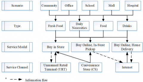
The features of new retailing depend on the specific scene. In different scenes, the consumers have vastly different types of demand, and also enjoy various options to fulfill their demand (Figure 1). New retailing offers two main kinds of terminals to satisfy consumer demand, namely, convenience stores (CSs) and unmanned retail terminals (URTs). The consumers choose between the terminals mainly based on their utilities [17].
Figure 1. The scenes and types of consumer demand and service models and channels in new retailing
2.1 Scene-based demand analysis for CSs
As shown in Figure $1,$ the CSs mainly satisfy the consumer demand for "buy in store" and that for "buy online, in-store pickup". Let $I$ be the set of all consumers, $J$ be the set of all CSs, and $K$ be the set of all types of goods. Then, the demand of consumer $i$ for type $k$ goods can be denoted as $d_{i k} .$
Here, two decision variables are defined, namely, $x_{j}$ and $y_{i j}$ Both decision variables are either 0 or $1 .$ If a consumer decides to buy in $\mathrm{CS} j,$ then $x_{j}=1 ;$ otherwise, $x_{j}=0 .$ If consumer $i$ decides to buy online and pick up the goods buy in CS $j,$ then $y_{i j}=1 ;$ otherwise $, y_{i j}=0$.
According to the concave-convex coverage function $a_{i j}$ proposed by Ghossoub et al. [18], the attraction between consumer i and CS j can be expressed as:
$a_{ij}=\left\{\begin{array}{ccc}{1 r_{i j} \leq L_{s}^{c}}\\{1-\left(\frac{r_{i j}-L_{s}^{c}}{U_{s}^{c}-L_{s}^{c}}\right)^{\eta_{i}} L_{s}^{c}<r_{i j}<U_{s}^{c}, \forall i \in I, j \in J}\\{0 r_{i j} \geq U_{s}^{c}}\end{array}\right.$ (1)
where, $r_{i j}$ is the distance between consumer $i$ and $\mathrm{CS} j ; L_{S}^{c}$ and $U_{s}^{c}$ are the minimum and maximum coverage distances of CSs in scene $s,$ respectively; $\eta_{i}$ is the distance sensitivity of consumer $i$
Then, the multinomial logit (MNL) model [ 19] was introduced to represent the random selection of consumers. The probabilities for consumer $i$ to choose "buy in store" $w_{i j}$ and "buy online, in-store pickup" $w_{i 0}$ can be respectively expressed as:
$w_{i j}=\frac{e^{\lambda \beta_{i j} a_{i j} x_{j}}}{1+\sum_{m \in J} e^{\lambda \beta_{i m} a_{i m} x_{m}}} i \in I, j \in J$ (2)
$w_{i 0}=\frac{1}{1+\sum_{m \in J} e^{\lambda u_{i m} x_{m}}} i \in I, j \in J$ (3)
where, $\beta_{i j}$ is the attraction of $\mathrm{CS} j$ to consumer $i ; \lambda$ is rationality degree of consumers. Thus, the total demand $D_{j}^{c}$ fulfilled by CS $j$ is the sum of the consumer demand for "buy in store" and that for "buy online, in-store pickup":
$D_{j}^{c}=\sum_{i \in I, k \in K} d_{i k}\left(w_{i j}+w_{i 0} y_{i j}\right) \forall j \in J$ (4)
2.2 Scene-based demand analysis for URTs
The URTs only partly fulfil the consumer demand for “buy in store”, due to the limited goods available on each terminal.
Here, a decision variable is defined, namely, $z_{j k} .$ The -lecision variable is either 0 or 1. If URT j provides type $k$ goods, then $Z_{j k}=1 ;$ otherwise $, Z_{j k}=0$
Suppose URT j can fully meet the demand of consumer $i$ for type $k$ goods. Then, the URT's attraction to the consumer only depends on distance:
$a_{ij}=\left\{\begin{array}{ccc}{1 r_{i j} \leq L_{s}^{t}}\\{1-\left(\frac{r_{i j}-L_{s}^{t}}{v_{s}^{t}-L_{s}^{t}}\right)^{\eta_{i}} L_{s}^{t}<r_{i j}<U_{s}^{t}, \forall i \in I, j \in J}\\{0 r_{i j} \geq U_{s}^{t}}\end{array}\right.$ (5)
where, $r_{i j}$ is the distance between consumer $i$ and URT $j ; L_{S}^{t}$ and $U_{s}^{t}$ are the minimum and maximum coverage distances of URTs in scene $s$, respectively.
According to the MNL model, the probability for consumer i to buy type k goods at URT j can be expressed as:
$W_{i j k}^{e}=\frac{e^{\lambda \delta_{i j k} a_{i j}} z_{j k}}{1+\sum_{m \in J, n \in K} e^{\lambda \delta_{i m n} a_{i m z_{m n}}}} i \in I, j \in J, k \in K$ (6)
where, $\delta_{i j k}$ is the attraction of URT $j,$ which provides type goods, to consumer $i$.
If URT $j$ fails to satisfy the demand of consumer $i,$ the consumer may give up the purchase or buy alternative goods. Let $(1-\pi)$ be the proportion of consumers giving up the purchase, i.e. the consumer loss ratio. For the remaining consumers $(\pi),$ the attraction from URT $j,$ which provides type $k$ goods, can be expressed as $\theta_{k} a_{i j},$ with $\theta_{k} \in(0,1)$ being the consumer satisfaction with the alternatives to type $k$ goods.
Hence, the probability $W_{i j k}^{r}$ for consumer $i$ to buy Iternatives to type $k$ goods at URT $j$ can be expressed as:
$W_{i j k}^{r}=\frac{e^{\lambda \delta_{i j k} \theta_{k} a_{i j}} z_{j k}}{1+\sum_{m \in J, n \in K} e^{\lambda \delta_{i m n} \theta_{n} a_{i m z_{m n}}}} i \in I, j \in J, k \in K$ (7)
Thus, the total demand $D_{j k}^{N}$ fulfilled by CS $j$ is to sum of the consumer demand for desired goods (type $k$ goods) and that for alternatives:
$D_{j k}^{N}=\sum_{i \in l}\left(d_{i k} W_{i j k}^{e}+\pi d_{i \hat{k}} W_{i j k}^{r}\right) \forall j \in J, k, \hat{k} \in K, \hat{k} \neq k$ (8)
3.1 Hypotheses
From the perspective of retailers, this paper focuses on optimizing the configuration of multi-type terminals in different scenes. The basic hypotheses were put forward as follows:
Hypothesis 1: All types of terminals have been replenished;
Hypothesis 2: The CSs have not capacity limit, fully satisfy consumer demand, and fulfil the demand for “buy online, in-store pickup”;
Hypothesis 3: The URTs have capacity limit, and the same type of goods are available on only one URT in the same scene;
Hypothesis 4: The demands of different consumers are independent of each other, and the demand of the same consumer can be fulfilled by multiple different terminals.
3.2 Objectives
In new retailing, cost optimization is no longer the only pursuit of the configuration of the logistics network. The fulfilment of consumer demand is of equal importance to retailers [20]. Therefore, our model was established from three dimensions: daily mean profit, consumer satisfaction and the number of terminals.
(1) Maximization of daily mean profit
The daily mean profit TP equals the difference between daily revenue TR and daily cost TC. The retailer’s revenue consists of sales revenue and the courier fees paid by online shopping consumers; the retailer’s cost includes the inventory costs of CSs and URTs, the rent of CSs, the purchase and operating expenses of URTs, as well as the distribution costs incurred by online shopping consumers. Hence, the daily revenue TR can be expressed as:
$T R=\sum_{i \in I, j \in J, k \in K}\left[p_{k}^{s}\left(D_{j}^{c}+D_{j k}^{N}\right)+p^{d} d_{i k} w_{i 0} y_{i j}\right]$ (9)
where, $p_{k}^{s}$ is the price of type $k$ goods; $p^{d}$ is the courier fees paid by online shopping consumers.
Meanwhile, the daily cost TC can be expressed as:
$T C=\sum_{i \in I, j \in J, k \in K}\left(\frac{1}{2} h_{j}^{C} D_{j}^{c}+\frac{1}{2} h_{j k}^{N} D_{j k}^{N}+c_{i j}^{d} d_{i k} w_{i 0} y_{i j}+\right.\left.o_{j}^{C} x_{j}+o^{N} z_{j k}\right)$ (10)
where, $h_{j}^{c}$ and $h_{j k}^{N}$ are the unit inventory costs of $\mathrm{CS} j$ and URT $j,$ respectively; $c_{i j}^{d}$ is the unit distribution cost between $\mathrm{CS} j$ and consumer $i ; o_{j}^{C}$ is the daily mean rent of $\mathrm{CS} j ; o^{N}$ is the purchase and operating expenses of URT $j$
Therefore, the maximization of the retailer’s daily mean profit can be described as:
$T P=\max (T R-T C)=\max \sum_{i \in I, j \in J, k \in K}\left[p_{k}^{S} d_{i k}\left(w_{i j}+w_{i 0} y_{i j}\right)+p_{k}^{S}\left(d_{i k} W_{i j k}^{e}+\right.\right.$
$\left.\pi d_{i \widehat{k}} W_{i j k}^{r}\right)+p^{d} d_{i k} w_{i 0} y_{i j}-\frac{1}{2} h_{j}^{C} d_{i k}\left(w_{i j}+w_{i 0} y_{i j}\right)-\left.\frac{1}{2} h_{j k}^{N}\left(d_{i k} W_{i j k}^{e}+\pi d_{i \hat{k}} W_{i j k}^{r}\right)-c_{i j}^{d} d_{i k} w_{i 0} y_{i j}-o_{j}^{C} x_{j}-o^{N} z_{j k}\right]$ (11)
(2) Maximization of consumer satisfaction
In new retailing, the consumer satisfaction with terminal configuration mainly depends on the product quantity, service punctuality, product price and product attributes. Drawing on the method proposed by Hoseinpour and Ahmadi-Javid [21], the consumer satisfaction was measured by four indices: effectiveness satisfaction $S_{1},$ time satisfaction $S_{2},$ cost satisfaction $S_{3}$ and product attribute satisfaction $S_{4} .$ The weights of the four indices, i.e. $v_{1}, v_{2}, v_{3}, v_{4},$ in consumer satisfaction satisfy $v_{1}+v_{2}+v_{3}+v_{4}=1$.
If a consumer chooses “buy in store” or “buy online, in-store pickup”, he/she can always find the desired goods within an affordable cost. His/her satisfaction is only affected by the time spent in shopping. The time satisfaction $S_{2}$ is related to the distance between the consumer and the CS, and can be described by the attraction function $a_{i j} .$ Thus, the overall satisfaction $T S^{C}$ of this type of consumers can be expressed as:
$T S^{C}=\sum_{i \in I, j \in J, k \in K}\left(v_{1}+v_{2} a_{i j}+v_{3}+v_{4}\right) d_{i k} w_{i j}$ (12)
If a consumer chooses “buy online, home delivery”, his/her satisfaction is influenced by the time and cost of shopping. The time satisfaction $S_{2}$ can still be described by the attraction function $a_{i j} .$ Meanwhile, the cost satisfaction $S_{3}$ mainly hinges on the ratio of courier fee to product price: $S_{3}=p_{k}^{S} / p^{d} .$ Then, the overall satisfaction $T S^{D}$ of this type of consumers can be expressed as:
$T S^{D}=\sum_{i \in I, j \in J, k \in K}\left(v_{1}+v_{2} a_{i j}+\frac{v_{3} p_{k}^{s}}{p^{d}}+v_{4}\right) d_{i k} w_{i 0}$ (13)
If a consumer accepts the service of URT and finds the desired goods, his/her satisfaction is only affected by the time spent in shopping. Hence, the overall satisfaction $T S^{N e}$ of this type of consumers can be expressed as:
$T S^{N e}=\sum_{i \in I, j \in J, k \in K}\left(v_{1}+v_{2} a_{i j}+v_{3}+v_{4}\right) d_{i k} W_{i j k}^{e}$ (14)
If a consumer accepts the service of URT but only finds the alternative goods, the indices affecting his/her satisfaction are $S_{1}=0, S_{2}=a_{i j}, \quad S_{3}=p_{k}^{S} / p_{\hat{k}}^{S}$ and $S_{4}=\theta k .$ The overall
satisfaction $T S^{N r}$ of this type of consumers can be expressed as:
$T S^{N r}=\sum_{i \in I, j \in J, k \in K}\left(v_{2} a_{i j}+\frac{v_{3} p_{k}^{S}}{p_{\hat{k}}^{S}}+v_{4} \theta_{k}\right) \pi d_{i \hat{k}} W_{i j k}^{r}$ (15)
To sum up, the maximization of the consumer satisfaction can be generalized as:
$T S=\max \left(T S^{C}+T S^{D}+T S^{N e}+T S^{N r}\right)$ (16)
(3) Minimization of the number of terminals
In addition to cost, the deployment and operation of terminals face numerous constraints and uncontrollable factors. On the premise of satisfying consumer demand, the management pressure of the retailer can be greatly relieved by minimizing the number of terminals, i.e. maximizing the coverage of each terminal. The minimization of the number of multi-type terminals can be expressed as:
$T N=\min \sum_{j \in J, k \in K}\left(x_{j}+z_{j k}\right)$ (17)
3.3 Multi-objective optimization model
Through the above analysis, a multi-objective optimization model was constructed for multi-type terminal configuration in different scenes of new retailing:
(P) $\left\{\begin{array}{l}{\text { Max TP }} \\ {\text { Max TS }} \\ {\text { Min TN }}\end{array}\right.$
s.t.
$\sum_{j \in J} D_{j}^{C}+\sum_{j \in J, k \in K} D_{j k}^{N} \geq \sum_{i \in I, k \in K} d_{i k}$ (18)
$D_{j k}^{N} \leq A_{k} \forall j \in J, k \in K$ (19)
$x_{j} \geq y_{i j} \forall i \in I, j \in J$ (20)
$x_{j}, y_{i j}, z_{j k} \in\{0,1\} \forall i \in I, j \in J, k \in K$ (21)
The objectives of the above model include the maximum daily mean profit of the retailer MaxTP, the maximum consumer satisfaction MaxTS and the minimum number of terminals MaxTN. Constraint (18) requires that the retailer’s daily supply should be greater than or equal to the daily consumer demand; Constraint (19) is the capacity limit of URTs, in which $A_{k}$ is the capacity for type k goods; Constraints (20) and (21) define the value intervals of different variables.
There are many ways to solve multi-objective optimization problems. The most common approach is to transform the model into a single-objective problem [22-24]. In our model, the objective function TN has a completely different structure from that of TP and TS, making it difficult to find a combinatory solution. Therefore, this paper presents a hybrid PSO-GA based on elite recombination and directed optimization (directed elite search). First, the initial solutions of the model were generated through optimum search in solution space. Then, the initial solutions were subjected to recombination and directional optimization by the hybrid PSO-GA, such as to iteratively approximate the global optimal solution of the model.
4.1 Generation of initial solutions
The two objectives TP and TS were combined into a single objective TPS, with the weights of $\phi_{1}$ and $\phi_{2},$ respectively. Then, the maximization of the TPS can be expressed as:
Max TPS $=\phi_{1} T P+\phi_{2} T S$ (22)
since $\frac{\partial^{2} \operatorname{TPS}}{\partial z_{j k}^{2}} \leq 0,$ there always exits a $z_{j k}$ that maximizes the TPS. Suppose $\frac{\partial \mathrm{TPS}}{\partial z_{j k}}=0,$ and we have:
$Z_{j k}=\frac{\left(\phi_{1} f_{3}+\phi_{2} g_{1}\right) d_{i k} E_{2} q_{2} q_{3}^{2}+\left(\phi_{1} f_{3}+\phi_{2} g_{3}\right) \pi d_{i \widehat{k}} E_{3} q_{3} q_{2}^{2}-\phi_{1} o^{N} q_{2}^{2} q_{3}^{2}}{\left(\phi_{1} f_{3}+\phi_{2} g_{1}\right) d_{i k} E_{2}^{2} q_{3}^{2}+\left(\phi_{1} f_{3}+\phi_{2} g_{3}\right) \pi d_{i \hat{k}} E_{3}^{2} q_{2}^{2}}$ (23)
where, $E_{2}=e^{\lambda \delta_{i j k} a_{i j}} ; \quad E_{3}=e^{\lambda \theta_{k} \delta_{i j k} a_{i j}} ; f_{3}=p_{k}^{S}-\frac{1}{2} h_{j k}^{N}; g_{1}=v_{1}+v_{2} a_{i j}+v_{3}+v_{4} ; g_{3}=v_{2} a_{i j}+\frac{v_{3} p_{k}^{S}}{p_{\vec{k}}^{s}}+v_{4} \theta_{k} ; q_{2}=1+\sum e^{\lambda \delta_{i m n} a_{i m}} z_{m n} ; q_{3}=1+\sum e^{\lambda \theta_{n} \delta_{i m n} a_{i m} Z_{m n}}$
From $\frac{\partial \mathrm{TPS}}{\partial x_{j}}=0,$ we have:
$x_{j}=\frac{q_{1}}{E_{1}}-\frac{\phi_{1} q_{1}^{2} o_{j}^{C}}{\left(\phi_{1} f_{1}+\phi_{2} g_{1}\right) E_{1}^{2} d_{i k}}-\frac{\phi_{1} f_{2}+\phi_{2} g_{2}}{\left(\phi_{1} f_{1}+\phi_{2} g_{1}\right) E_{1}} y_{i j}$ (24)
where, $E_{1}=e^{\lambda \beta_{i j} a_{i j}} ; q_{1}=1+\sum e^{\lambda \beta_{i m} a_{i m}} x_{m} ; f_{1}=p_{k}^{S}-$$\frac{1}{2} h_{j}^{C} ; f_{2}=p_{k}^{S}-\frac{1}{2} h_{j}^{C}+p^{d}-c_{i j}^{d} ; g_{2}=v_{1}+v_{2} a_{i j}+\frac{v_{3} p_{k}^{S}}{p^{d}}+v_{4}$
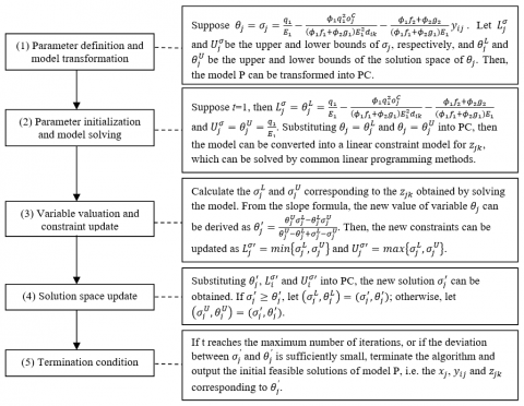
As shown in formula $(24),$ the $x_{j}$ that leads to the optimal TPS is always related to $y_{i j} .$ since $\frac{\partial \mathrm{TPS}}{\partial y_{i j}}=\frac{\phi_{1} f_{2}+\phi_{2} g_{2}}{q_{1}} d_{i k}$ is constant, it is very difficult to identify the optimal solution directly. To overcome this difficulty, this paper puts forward an initial solution generation method based on optimum search in solution space. The workflow of the optimum search algorithm is illustrated in Figure 2. First, a new optimization model was constructed with MinTN as the objective function. Taking the $x_{j}$ that leads to the optimal TPS as the independent variable, the corresponding $z_{j k}$ and $\mathrm{TN}$ were solved by formula ( 23) and the constraints of the original multi-objective optimization model. Then, the TN was minimized by continuously adjusting the search range of $x_{j} .$ The corresponding $x_{j}$ and $z_{j k}$ are the initial feasible solutions that satisfy Min TN and Max TPS at the same time.
The optimum search algorithm can be expressed as:
$(\mathrm{PC}) \mathrm{MIN} T N=L Z+\sum_{j \in J} \theta_{j}$
s.t. formulas (18) -(21)
$L Z=\sum_{j \in J, k \in K} z_{j k}\left(\theta_{j}\right)$
$\frac{q_{1}}{E_{1}}-\frac{\phi_{1} q_{1}^{2} o_{j}^{C}}{\left(\phi_{1} f_{1}+\phi_{2} g_{1}\right) E_{1}^{2} d_{i k}}-\frac{\phi_{1} f_{2}+\phi_{2} g_{2}}{\left(\phi_{1} f_{1}+\phi_{2} g_{1}\right) E_{1}} y_{i j} \geq L_{j}^{\sigma}$
$\frac{q_{1}}{E_{1}}-\frac{\phi_{1} q_{1}^{2} o_{j}^{C}}{\left(\phi_{1} f_{1}+\phi_{2} g_{1}\right) E_{1}^{2} d_{i k}}-\frac{\phi_{1} f_{2}+\phi_{2} g_{2}}{\left(\phi_{1} f_{1}+\phi_{2} g_{1}\right) E_{1}} y_{i j} \leq U_{j}^{\sigma}$
Figure 2. Optimum search algorithm for initial solutions
4.2 Search for global optimal solution
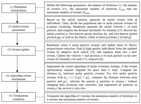
The GA has been widely adopted to solve multi-objective models, thanks to its advantages of parallel search and adaptive adjustment. Nonetheless, this algorithm has problems like premature convergence and low operating efficiency [25]. To address these problems, this paper designs a hybrid PSO-GA (Figure 3), which updates the swarm of the GA through rapid iterations of the PSO and restarts whenever the optimization process is stagnant. This hybrid algorithm can converge to high-quality solutions at a fast speed.
The hybrid PSO-GA can be expressed as:
$l=l_{1}-\frac{\left(l_{1}-l_{2}\right)}{T_{\max }} k$ (25)
$w_{i}^{k}=w_{i}^{0}+\varepsilon_{0} \frac{f_{i}^{k}-f_{\min }^{k}+\delta_{0}}{f_{\max }^{k}-f_{\min }^{k}+\delta_{1}} \cdot \frac{T_{\max }-k}{T_{\max }}$ (26)
$v^{k+1}=w_{i}^{k} v^{k}+\varepsilon_{1}\left(b p^{k}-p^{k}\right)+\varepsilon_{2}\left(g p^{k}-p^{k}\right)$ (27)
$p^{k+1}=p^{k}+v^{k+1}$ (28)
where, $l_{1}$ and $l_{2}$ are the maximum and minimum of the preset distance threshold, respectively; $w_{i}^{k}$ is the inertia weight of particle $i$ in the $k$ -th iteration; $w_{i}^{0}$ is the preset weight of particle $i ; f_{\max }^{k}$ and $f_{\min }^{k}$ are the maximum and minimum fitness of particles in the $k$ -th iteration; $\varepsilon$ and $\delta$ are factor adjustment coefficients, both of which are random numbers in [0,1].
Figure 3. The hybrid PSO-GA
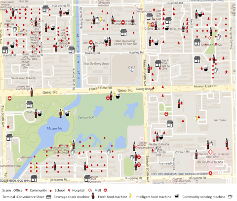
To verify its effectiveness, the proposed strategy was applied to analyze the terminal configuration of a department store in a region, including such scenes as office, community, school, hospital and mall. Four types of URTs are involved: beverage snack machine, fresh food machine, intelligent food machine, and commodity vending machine.
5.1 Parameter setting
The consumer demand at each place is the product between population and consumption power index. The population is assumed to be evenly distributed across this region, and positively correlated with the building area at each place. Besides, the consumption power index changes from scene to scene. In office and community, the consumption power index depends on the selling price per unit area.
The daily mean rent and operating expense of the CSs are related to the location and the type of surrounding scenes, and were obtained through surveys: $p_{k}^{S} \in U[2,15], p^{d} \in U[3,8]$ $h_{j}^{C} \in U[0.5,1.5], h_{j k}^{N} \in U[1,2],$ and $O^{N} \in U[20,30] .$ Different types of terminals vary in coverage distance. The minimum and maximum coverage distances of the CSs were set to $L_{s}^{c} \in$ $U[0.3,0.6]$ and $U_{s}^{c} \in U[1,1.3],$ respectively; the minimum and maximum coverage distances of the URTs were set to $L_{s}^{t} \in$ $U[0.1,0.4]$ and $U_{s}^{t} \in U[0.4,0.8],$ respectively.
The other parameters were configured as follows: $\rho \in$ $U[0.1,0.3], \eta \in U[0.5,1.5], \beta \in U[1,5], \delta \in U[1,5], \lambda \in$$U[4,6], \theta \in U[0.3,0.8], \pi \in U[0.4,0.6], v_{1}=0.3, v_{2}=0.2, v_{3}=0.3, v_{4}=0.2, \phi_{1}=\phi_{2}=0.5,$ maximum number of searches in the solution space $T=30,$ target deviation $\varepsilon=0.01,$ the maximum number of iterations of the hybrid PSO-GA $N_{\max }=20,$ the maximum number of restarts
$N_{\max }=20,$ the swarm size $Q=100,$ the number of niche particle swarms $m=5,$ and the number of steps of optimization stagnation $\pi=5$
5.2 Results analysis
Through calculation, a total of 76 multi-type terminals were deployed in the region, including 14 CSs, 32 beverage snack machines, 7 fresh food machines, 12 intelligent food machines and 11 commodity vending machines. The location of each terminal is shown in Figure 4.
(1) Influence of terminal type on decision-making
The multi-type terminal model was compared with the CS-only and the URT-only models in terms of their influence on decision-making. As shown in Table 1, the multi-type terminal model boasts the highest daily mean profit, surpassing that of the CS-only model and the URT-only model by 13.7% and 39.1%, respectively. By contrast, the consumer satisfaction and number of terminals in the multi-type terminal model were on the medium levels, lower than those of the URT-only model. If the retailer vigorously pursues profit, the multi-type terminal model is the best option; if the retailer stresses on service quality, it should increase the number of URTs in demand-concentrated places.
Figure 4. Configuration of multi-type terminals based on scenes
Table 1. Comparison between terminal configuration models
|
|
Multi-type terminals |
CS-only |
URT-only |
|
TP |
39,550 |
34,796 |
28,441 |
|
TS |
165 |
124 |
186 |
|
TN |
76 |
22 |
105 |
Three URT configuration strategies were compared to disclose the influence of scene on decision-making: only beverage snack machines are deployed in each scene (single strategy), different URTs are deployed in different scenes (differentiated strategy), and all four types of URTs are deployed in each scene (complete strategy). As shown in Table 2, the differentiated strategy outperformed the single strategy in both daily mean profit (>20.2%) and consumer satisfaction (>47.3%). Compared with the complete strategy, the differentiated strategy achieved a low consumer satisfaction (<5.2%) but a very high daily mean profit (>53.4%). Overall, the differentiated strategy, which fully considers the scenes, reduces the profit loss caused by short supply, and also lowers the cost and management difficulty resulted from idle terminals.
Table 2. Comparison between different URT configuration strategies
|
|
Differentiated strategy |
Single strategy |
Complete strategy |
|
TP |
39,550 |
32,890 |
25,788 |
|
TS |
165 |
112 |
174 |
|
TN |
76 |
68 |
138 |
Sensitivity analysis aims to reflect how optimization objectives change with the parameter values. Considering the difference in metric unit between the three objectives, the variation in each objective was calculated by adjusting the values of key parameters, with the optimal configuration was taken as the benchmark.
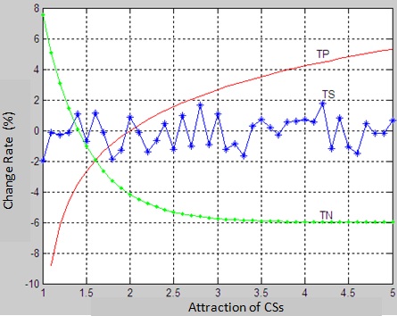
Figure 5 and Figure 6 illustrate how the three objectives correlate with the attractions $\beta$ and $\delta$ of the CSs and the URTs to consumers, respectively. It can be seen that the greater the attraction, the higher the daily mean profit; the attraction of the CSs is negatively correlated with the total number of terminals, but unrelated to consumer satisfaction; the attraction of the URTs has a positive correlation with consumer satisfaction. As a result, any retailer looking for profit and consumer satisfaction should improve the attraction of retail terminals, especially the URTs, to consumers.
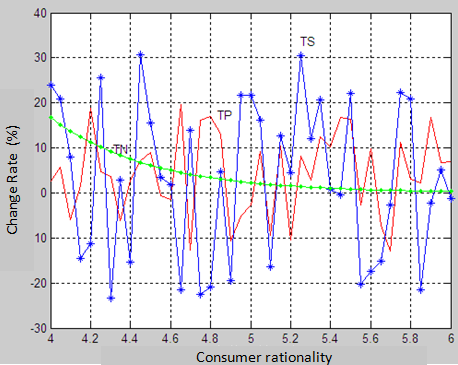
Figure 7 presents the influence of consumer rationality on the three objectives. With the growing rationality of consumers, the retailer needs fewer and fewer terminals to fulfil the consumer demand, while daily mean profit and consumer satisfaction did not exhibit a clear trend. Thus, the retailer should cautiously analyze the rationality of regional consumers, before making the optimal decision on the configuration of retail terminals.
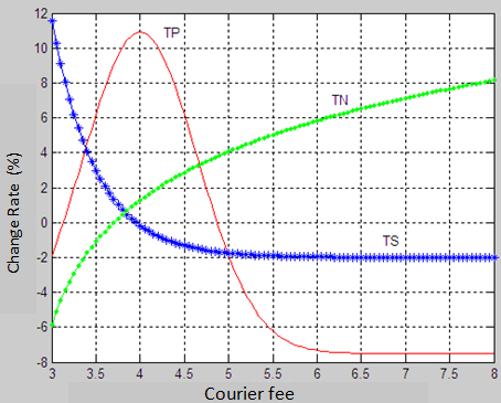
Among the cost parameters, rent and inventory cost are inevitable expenditures for the retailer, while the courier fee is controllable by the retailer. As shown in Figure 8, with the growth in the courier fee, the consumer satisfaction decreased, the number of terminals needed increased, while the daily mean profit first increased, then declined and eventually stabilized. To strike a balance between profit and consumer satisfaction, the retailer must find the optimal balance point in the courier fee.
Figure 5. The relationship between the three objectives and the attraction of the CSs to consumers
Figure 6. The relationship between the three objectives and the attraction of the URTs to consumers
Figure 7. The relationship between the three objectives and consumer rationality
Figure 8. The relationship between the three objectives and courier fee
Retail terminals are close to consumers, and directly satisfy their demand. In new retailing, these terminals are the key nodes in the last-mile service network. The type, number, location and coverage of retail terminals have a direct bearing on the service quality and profit level of the retailer. Therefore, this paper probes deep into the multi-objective decision-making model for the optimal configuration of multi-type terminals based on scenes, and designs a hybrid PSO-GA based on directed elite search to solve the decision-making model. Empirical results demonstrate the feasibility of our model and algorithm. It is concluded that the retail terminals should be configured by improving their attraction, cautiously analyzing consumer rationality and properly setting the courier fee.
[1] Global Retail Alliance. Global Powers of Retailing 2019 [EB/OL]. https://www.gra.world/global-powers-of-retailing-2019/, 2019-2-3.
[2] Nilsson, P. (2016). The influence of related and unrelated industry diversity on retail firm failure. Journal of Retailing and Consumer Services, 28: 219-227. https://doi.org/10.1016/j.jretconser.2015.09.006
[3] Grewal, D., Roggeveen, A.L., Nordfalt, J. (2017). The Future of Retailing. Journal of Retailing, 93(1): 1-6. https://doi.org/10.1016/j.jretai.2016.12.008
[4] Janjevic, M., Winkenbach, M., Merchán, D. (2019). Integrating collection-and-delivery points in the strategic design of urban last-mile e-commerce distribution networks. Transportation Research Part E: Logistics and Transportation Review, 131: 37-67. https://doi.org/10.1016/j.tre.2019.09.001
[5] Castillo, V.E., Bell, J.E., Rose, W.J., Rodrigues, A.M. (2017). Crowdsourcing last mile delivery: Strategic implications and future research directions. Journal of Business Logistics, 39(1): 1-79. https://doi.org/10.1111/jbl.12173
[6] Iwan, S., Kijewska, K., Lemke, J. (2016). Analysis of parcel lockers’ efficiency as the last mile delivery solution – the results of the research in Poland. Transportation Research Procedia, 12: 644-655. https://doi.org/10.1016/j.trpro.2016.02.018
[7] Wollenburg, J., Hübner, A., Kuhn, H., Trautrims, A. (2018). From bricks-and-mortar to bricks-and-clicks. International Journal of Physical Distribution & Logistics Management, 48(4): 415-438. https://doi.org/10.1108/IJPDLM-10-2016-0290
[8] Wollenburg, J., Holzapfel, A., Hübner, A., Kuhn, H. (2018). Configuring retail fulfillment processes for omni-channel customer steering. International Journal of Electronic Commerce, 22(4): 540-575. https://doi.org/10.1080/10864415.2018.1485085
[9] Xu, J.J., Cao, L.L. (2019). Optimal in-store inventory policy for omnichannel retailers in franchising networks. International Journal of Retail & Distribution Management, 47(12): 1251-1265. https://doi.org/10.1108/IJRDM-09-2018-0199
[10] Liu, K.J., Zhou, Y.H., Zhang, Z.G. (2010). Capacitated location model with online demand pooling in a multi-channel supply chain. European Journal of Operational Research, 207(1): 218-231. https://doi.org/10.1016/j.ejor.2010.04.029
[11] Chen, G., Daskin, M.S., Shen, Z.J.M., Uryasev, S. (2010). The α-reliable mean-excess regret model for stochastic facility location modeling. Naval Research Logistics, 53(7): 617-626. https://doi.org/10.1002/nav.20180
[12] Aboolian, R., Berman, O., Krass, D. (2007). Competitive facility location model with concave demand. European Journal of Operational Research, 181(2): 598-619. https://doi.org/10.1016/j.ejor.2005.10.075
[13] Karatas, M. (2017). A multi-objective facility location problem in the presence of variable gradual coverage performance and cooperative cover. European Journal of Operational Research, 262(1): 1040-1051. https://doi.org/10.1016/j.ejor.2017.04.001
[14] Pishvaee, M.S., Farahani, R.Z., Dullaert, W. (2010). A memetic algorithm for bi-objective integrated forward/reverse logistics network design. Computers & Operations Research, 37(6): 1100-1112. https://doi.org/10.1016/j.cor.2009.09.018
[15] Pasandideh, S.H.R., Niaki, S.T.A., Hajipour, V. (2013). A multi-objective facility location model with batch arrivals: two parameter-tuned meta-heuristic algorithms. Journal of Intelligent Manufacturing, 24(2): 331-348. https://xs.scihub.ltd/https://doi.org/10.1007/s10845-011-0592-7
[16] Govindan, K., Paam, P., Abtahi, A.R. (2016). A fuzzy multi-objective optimization model for sustainable reverse logistics network design. Ecological Indicators, 67: 753-768. https://doi.org/10.1016/j.ecolind.2016.03.017
[17] Murfield, M., Boone, C.A., Rutner, P., Thomas, R. (2017). Investigating logistics service quality in omni-channel retailing. International Journal of Physical Distribution & Logistics Management, 47(4): 263-296. https://doi.org/10.1108/IJPDLM-06-2016-0161
[18] Ghossoub, M. (2019). Optimal insurance under rank-dependent expected utility. Insurance: Mathematics and Economics, 87: 51-66. https://doi.org/10.1016/j.insmatheco.2019.04.005
[19] Agrawal, S., Avadhanula, V., Goyal, V., Zeevi, A. (2019). MNL-bandit: A dynamic learning approach to assortment selection. Operations Research, 67(5): 1209-1502. https://doi.org/10.1287/opre.2018.1832
[20] Hong, I.B. (2017). Predicting user-level marketing performance of location-based social networking sites. Journal of Computer Information Systems, 262(1): 1040-1051. https://doi.org/10.1080/08874417.2018.1435318
[21] Hoseinpour, P., Ahmadi-Javid, A. (2016). A profit-maximization location-capacity model for designing a service system with risk of service interruptions. Transportation Research Part E: Logistics and Transportation Review, 96: 113-134. https://doi.org/10.1016/j.tre.2016.08.004
[22] Mirjalili, S.Z., Mirjalili, S., Saremi, S., Faris, H., Aljarah, I. (2018). Grasshopper optimization algorithm for multi-objective optimization problems. Applied Intelligence, 48(4): 805-820. https://xs.scihub.ltd/https://doi.org/10.1007/s10489-017-1019-8
[23] Zareizadeh, Z., Helfroush, M.S., Rahideh, A., Kazemi, K. (2018). A robust gene clustering algorithm based on clonal selection in multiobjective optimization framework. Expert Systems with Applications, 113(15): 301-314. https://doi.org/10.1016/j.eswa.2018.06.047
[24] Mirjalili, S., Jangir, P., Mirjalili, S.Z., Saremi, S., Trivedi, I.N. (2017). Optimization of problems with multiple objectives using the multi-verse optimization algorithm. Knowledge-Based Systems, 134(15): 50-71. https://doi.org/10.1016/j.knosys.2017.07.018
[25] Mousavi-Avval, S.H., Rafiee, S., Sharifi, M.B., Hosseinpour, S., Notarncola, B., Tassielli, G., Renzulli, P. (2017). Application of multi-objective genetic algorithms for optimization of energy, economics and environmental life cycle assessment in oilseed production. Journal of Cleaner Production, 140(1): 804-815. https://doi.org/10.1016/j.jclepro.2016.03.075
[26] Dell’Amico, M., Díaz, J.C.D., Hasle, G., Iori, M. (2016). An adaptive iterated local search for the mixed capacitated general routing problem. Transportation Science, 50(4): 1139-1393. https://doi.org/10.1287/trsc.2015.0660