Weiliang Zhang | Mingjun Liu | Xin Wang*
OPEN ACCESS
The purpose of this study was to overcome the defects of existing road maintenance vehicles, the approach designs a new road maintenance vehicle with a multi-working position manipulator and an automatic feeding mechanism was adopted, the end of the manipulator was installed an indexable maintenance equipment, which integrates multiple functions like cutting, milling and pouring, all functions are driven by the same power source. During the maintenance, the indexable maintenance equipment can switch between different functions. In addition, an automatic feeding mechanism and a hot mix asphalt (HMA) heating and mixing system were set up to recover and reuse the waste generated in the maintenance. Finally, the parameters of the key parts of the vehicle were designed and calculated, yielding the final overall design of the road maintenance vehicle. The results indicated that this device can ensure that the physical consumption of lifting and maintenance equipment is reduced to the greatest extent during the construction process. The impacts of the obtained results are guarantee the construction process is safer and faster, the degree of automation in the construction process is higher, and workers are also kept away from the harsh construction environment.
automatic feeding mechanism, road maintenance vehicle, manipulator, hot mix asphalt (HMA), HMA heating and mixing system
Over the years, road maintenance has become more and more difficult and labor-consuming, so automation in road construction and maintenance is currently actively developing in the United States, China and other countries in the world. In order to solve the problem of high maintenance efficiency and low cost, maintenance equipment with high degree of automation and good maintenance efficiency is required [1-3].
In terms of the need to lift the onboard devices during maintenance, some scholars design a special lifting device for road maintenance vehicles, and analyzes the layout and stress of the lifting device [4]. According to the maintenance requirements in plateau areas, a multifunctional maintenance vehicle equipped with small maintenance equipment is designed [5]. Ma et al. [6] puts forward a comprehensive road maintenance vehicle with good integration and reasonable configuration, using the theory of inventive problem solving (TRIZ). Nevertheless, many of the existing road maintenance vehicles require workers to clean the target pits and cracks using onboard crusher, cutter and blower, fill the hot mix asphalt (HMA) or cold feed, and then compact the road repeatedly with the onboard compactor. There are many defects with this maintenance strategy: (1) The complicated maintenance process has many hidden safety hazards related to the frequent lifting of onboard maintenance devices; (2) The onboard maintenance devices, which cause strong vibration and heavy dust, must be operated manually, posing serious damages to workers’ health; (3) The power between onboard maintenance devices has not been fully optimized, leading to redundant power sources and resource waste [7-12].
To solve the problems, this article designs an indexable maintenance equipment that integrates multiple functions (e.g. cutting, pouring, milling and high-pressure cleaning) at the end of the manipulator. The design attempts to provide the same power source to all maintenance devices, and ensure that the indexable vehicle can switch between different working positions as per the maintenance need. In addition, the following systems were set up to treat common road diseases: HMA heating and mixing system, waste crushing and recycling system, automatic feeding mechanism and asphalt heating and insulation system. The indexable equipment, coupled with the four systems, form a novel road maintenance vehicle.
In order to accomplish the above tasks, Firstly, this article designs the functional principle of highway maintenance vehicle. Secondly, it designs and calculates the parameters of key components, determines the parameters of the end manipulator, and determines the parameters of the mixing device through fluid simulation. Finally, the overall layout design of highway maintenance vehicles is completed.
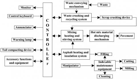
The functional design of the proposed road maintenance vehicle is illustrated in Figure 1. It can be seen that the waste generated in the construction is firstly crushed in the “waste crushing and recycling system”, and then transmitted to the “HMA heating and mixing system” to fully mix with hot asphalt; the HMA will be delivered to the maintenance area for secondary use. The hot asphalt for pouring and mixing comes from the “asphalt heating and insulation system”. Moreover, the “indexable maintenance equipment”, which integrates such working positions as pouring, cutting, milling and cleaning, can switch between different working positions under the control of the “manipulator”. The entire process is controlled by the controller and the keyboard and displayed on the monitor.
Figure 1. Functional design of the proposed road maintenance vehicle
3.1 Manipulator parameters and end trajectory analysis
The manipulator parameters affect the end trajectory, which in return determines whether the manipulator can work effectively. The more rational its parameters, the wider the effective working range of the manipulator. To eliminate the motion interference, it is necessary to fully analyze the end trajectory.
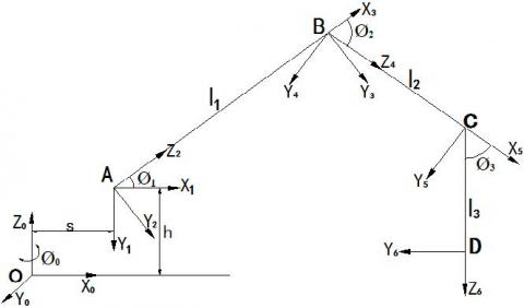
Our manipulator is a six-degree-of-freedom (6DOF) mechanism of three segments, in which the third segment is telescopic. The three segments are hinged to a turntable. Figure 2 shows the kinematics model of the manipulator established by the Denavit–Hartenberg (D-H) method. In the figure, $z_0, z_1, z_3$ and $z_5$ are joints rotating about the joint axis, and $z_2, z_4$ and $z_6$ are joints moving along the joint length. The D-H parameters of each joint is listed in Table 1 [13~15].
Figure 2. Kinematics model of the manipulator
Table 1. D-H parameters of the manipulator
|
Joint number |
1 |
2 |
3 |
4 |
5 |
6 |
|
Joint angle $\theta_{i}$ |
$\phi_{0} \phi_{0_0}$ |
$\phi_{0_{1}}$ |
0 |
$-\phi_{0_{2}}$ |
0 |
$-\phi_{0_{3}}$ |
|
Rod length |
0 |
0 |
$l_{1}$ |
0 |
$l_{2}$ |
$l_{3}$ |
|
Torsional angle $\alpha_{i}$ |
$90^{\circ}$ |
- $90^{\circ}$ |
$90^{\circ}$ |
- $90^{\circ}$ |
$90^{\circ}$ |
$90^{\circ}$ |
According to the joint parameters (Table 1) and the kinematics model (Figure 2), the transformation matrix $A_i$ from the i-th joint to the i-1-th joint can be established as:
$A_{1}=\operatorname{Rot}\left(Z_{0}, \phi_{0}\right) \operatorname{Tr} a n s(0,0, h) \operatorname{Tr} a n s(s, 0,0) \operatorname{Rot}\left(X_{1}, 90^{\circ}\right)$
$A_{2}=\operatorname{Rot}\left(Z_{1}, \phi_{1}\right) \operatorname{Rot}\left(Y_{2},-90^{\circ}\right),$
$A_{3}=\operatorname{Tr} \operatorname{ans}\left(0,0, l_{1}\right) \operatorname{Rot}\left(Y_{3}, 90^{\circ}\right)$
$A_{4}=\operatorname{Rot}\left(Z_{3},-\phi_{2}\right) \operatorname{Rot}\left(Y_{4},-90^{\circ}\right)$
$A_{5}=\operatorname{Trans}\left(0,0, l_{2}\right) \operatorname{Rot}\left(Y_{5}, 90^{\circ}\right)$
$A_{6}=\operatorname{Rot}\left(Z_{5},-\phi_{3}\right) \operatorname{Rot}\left(Y_{6},-90^{\circ}\right) \operatorname{Tr} \operatorname{ans}\left(0,0, l_{3}\right)$
where, $\theta_{123}=\phi_{3}+\phi_{2}-\phi_{1} ; \theta_{12}=\phi_{2}-\phi_{1}$.
By the D-H method, the end posture of a member can be obtained by the transformation matrix $^{0} T_{n}=\prod_{n=0}^{n} i-1 A_{i}$, where, $^{0} T_{n}$ is the function of such variables as $\phi_{1}, \phi_{2}$ and $\phi_{3}$ and $i-1 A_{i}=\left[\begin{array}{cc}{{^i-1}R_i} & {^{i-1}P_{i}} \\ {0} & {1}\end{array}\right]$ is the transformation matrix from the i-th coordinate system to the i-1-th coordinate system ($^{(i-1)} R_{i}$ is the posture matrix; $^{i-1} P$ is the position matrix). In this way, the position of the manipulator’s end relative to the fixed coordinate system $z_0$ can be constructed as:
$\left\{\begin{aligned} X_{D}=& \cos \phi_{0}\left[s+l_{1} \cos \phi_{1}+l_{2} \cos \theta_{12}+l_{3} \cos \theta_{123}\right] \\ Y_{D}=\sin \phi_{0}\left[s+l_{1} \cos \phi_{1}+l_{2} \cos \theta_{12}+l_{3} \cos \theta_{123}\right] \\ Z_{D}=h+l_{1} \sin \phi_{1}+l_{2} \sin \theta_{12}-l_{3} \sin \theta_{123} \end{aligned}\right.$ (1)
The speed at any point in the coordinate system relative to the fixed coordinate system $z_0$ can be calculated by:
$\frac{d^{0} p}{d t}=\left(\sum_{j=1}^{i} \frac{\partial^{0} A_{i}}{\phi_{i}}\right)$ $^ip; i=1,2 \cdots, n$ (2)
Thus, the speed of the manipulator’s end relative to fixed coordinate system $z_0$ at $ϕ_0=0$ can be determined as:
$\left\{\begin{array}{l}{\dot{X}_{D}=-l_{1} \dot{\phi}_{1} \sin \phi_{1}-l_{2}\left(\dot{\phi}_{2}-\dot{\phi}_{1}\right) \sin \left(\phi_{2}-\phi_{1}\right)} \\ {\dot{z}_{D}=l_{1} \dot{\phi}_{1} \cos \phi_{1}-l_{2}\left(\dot{\phi}_{2}-\dot{\phi}_{1}\right) \cos \left(\phi_{2}-\phi_{1}\right)}\end{array}\right.$ (3)
The acceleration of any point in the coordinate system relative to the fixed coordinate system $z_0$ can be calculated by:
$\frac{d^{20} p}{d t^{2}}=\left(\sum_{j=1}^{i} \frac{\partial^{20} A_{i}}{\phi_{j}^{2}} \ddot{\phi}_{j}\right)$ $^ip; i=1,2 \cdots, n$ (4)
hence, the acceleration of the manipulator’s end relative to fixed coordinate system $z_0$ at $ϕ_0=0$ can be determined as:
$\left\{\begin{aligned} \ddot{X}_{D} &=-l_{1} \ddot{\phi}_{1} \cos \phi_{1}-l_{2}\left(\ddot{\phi}_{2}-\ddot{\phi}_{1}\right) \cos \left(\phi_{2}-\phi_{1}\right) \\ \ddot{Z}_{D} &=l_{1} \ddot{\phi}_{1} \sin \phi_{1}+l_{2}\left(\ddot{\phi}_{2}-\ddot{\phi}_{1}\right) \sin \left(\phi_{2}-\phi_{1}\right) \end{aligned}\right.$ (5)
Since the levelling device guarantees the perpendicularity of $l_3$ to the ground, the manipulator movement must satisfy the angular relationship of $ϕ_3=90+ϕ_1-ϕ_2$. The end trajectory of the manipulator in the X-Z plane is shown in Figure 3 below.
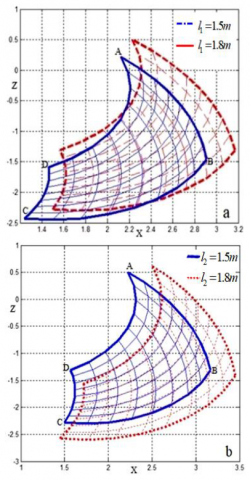
Figure 3. End trajectory of the manipulator in the X-Z plane ($l_1,l_2$ take different values)
As shown in Figure $3(a),$ when the first section length $l_{1}=1.8 m,$ second section length $l_{2}=1.5 m$ and third telescopic section length $l_{3}=2 m,$ the end trajectory of the manipulator is segment $A-B$ at $\phi_{2}=130^{\circ}$ and $\varphi_{1} \in 30^{\circ} \sim 70^{\circ},$ segment $C-D$ at $\phi_{2}=50^{\circ}$, and $\varphi_{1} \in 30^{\circ} \sim 70^{\circ},$ segment $B-C$ at $\phi_{1}=30^{\circ}$ and $\phi_{2} \in 50^{\circ} \sim 130^{\circ}$ , and segment $A-D$ at $\phi_{1}=70^{\circ}$ and $\phi_{2} \in 50^{\circ} \sim 130^{\circ}$ .
In Figure 3(a), $l_1=1.8min$ the dotted line and $l_1=1.5m$ in the solid line. It can be seen that, with the reduction in the $l_1$, the manipulator trajectory moves towards the negative direction of the Z axis and the X axis, indicating that the compaction roller is more likely to interfere in the manipulator movement at a smaller $l_1$. In Figure 3(b), $l_2=1.8m$ in the dotted line and $l_2=1.5m$ in the solid line. It can be seen that, with the reduction in the $l_2$, the manipulator trajectory moves towards positive direction of the Z axis and the X axis, indicating that a large $l_2$ promotes maintenance and suppresses interference.
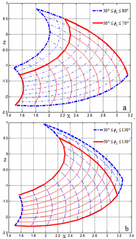
In Figure 4, the lengths of the first section, the second section and the third telescopic section are $l_1=1.8m$, $l_2=1.5m$ and $l_3=2m$, respectively, and $ϕ_2$ changes between 50° and 130°. Figure 4(a), where $30°≤ϕ_1≤70°$ in the solid line and $30°≤ϕ_1≤80°$ in the dotted line, shows that the increase in the upper bound of $ϕ_1$ does not promote the effective motion trajectory of the manipulator. Figure 4(b), where $50°≤ϕ_2≤130°$ in the solid line and $50°≤ϕ_2≤130°$ in the dotted line, shows that the increase in the lower bound of $ϕ_2$ does not promote the effective motion trajectory of the manipulator.
Figure 4. End trajectory of the manipulator in the X-Z plane (ϕ_1,ϕ_2 take different values)
Figure 5. End trajectory of the manipulator in the X-Y-Z plane (angle of the compaction swing rod take different values)
In Figure 5(a), the swing angle $ϕ_0$ of the rotary table changes between -30° and 30°, the lengths of the first section, the second section and the third telescopic section are $l_1=1.8m$, $l_2=1.5m$ and $l_3=2m$, respectively, the length and radius of the compaction roller are 0.78m and 0.28m, respectively, while the length and swing angle of the compaction swing rod are 1.5m and 20°, respectively. In this case, the compaction roller is retracted. In addition, the origin of the coordinate system is 1.5m above ground. It can be seen from Figure 5(a) that the lowest point of the compaction roller is greater than 0.7m from the ground, which does not hinder the normal movement.
In Figure 5(b), all the parameters are the same as in Figure 5(a), except for the swing angle of the compaction swing rod (60°). In this case, the compaction roller is at the working position for compaction. The origin of the coordinate system is still 1.5m above ground. It can be seen from Figure 5(b) that the compaction roller (Figure 4) is in contact with the target road, exerting no interference in the manipulator trajectory.
Figure 6. End trajectory of the manipulator in the X-Y-Z plane (radius of the compaction roller takes different values)
In Figure 6(a), the swing angle ϕ_0 of the rotary table changes between -60° and 60°, the lengths of the first section, the second section and the third telescopic section are $l_1=1.8m$, $l_2=1.5m$ and $l_3=1.5m$, respectively, the length and radius of the compaction roller are 2m and 0.35m, respectively, while the length and swing angle of the compaction swing rod are 1.5m and 60°, respectively. In this case, the compaction roller is in contact with the ground. It can be seen from Figure 6(a) that the compaction roller interferes in the manipulator trajectory. Specifically, the manipulator trajectory is shifted by 0.5m to the positive direction of Z axis, due to the reduction of the length of the third telescopic section $l_3$, and expands in the Y-direction thanks to the growth in the swing angle $ϕ_0$ of the rotary table.
In Figure 6(b), the swing angle ϕ_0 of the rotary table changes between -60° and 60°, the lengths of the first section, the second section and the third telescopic section are $l_1=1m$, $l_2=0.8m$ and $l_3=1.5m$, respectively, the length and radius of the compaction roller are 2m and 0.35m, respectively, while the length and swing angle of the compaction swing rod are 1.5m and 20°, respectively. In this case, the compaction roller is still in contact with the ground. It can be seen from Figure 6(b) that the compaction roller clearly interferes in the manipulator trajectory. The manipulator moves in a smaller range and its trajectory shifts towards the positive direction of the X axis, because of the shortening of the first and second sections.
Table 2. Motion parameters of the manipulator
|
Projects |
l1/m |
l2/m |
l3/m |
f1/° |
f1/° |
|
Size |
1.8 |
1.5 |
1.5~2 |
30~70 |
50~130 |
According to the above analysis results, the swing angle and length of the compaction swing rod were determined as 20°~60° and 1.5m, respectively, and the length and radius of the compaction roller were selected as 0.78m and 0.28m, respectively. The final parameters of the manipulator are listed in Table 2.
3.2 Mathematical model for manipulator kinematics
Using the Lagrangian method, the manipulator’s dynamics equation can be expressed as:
$T_{i}=\sum_{j=1}^{n} K_{i j}(\phi) \dot{\phi}_{i j}+\sum_{j=1}^{n} \sum_{t=1}^{n} H_{i j t}(\phi) \dot{\phi}_{j} \dot{\phi}_{t}+G_{i}(\phi)$ (6)
where, $T_i$ is the driving force acting on the manipulator; $K_{ij}(ϕ)$ is the moment of inertia of the manipulator; $H_{ijt}(ϕ)$ is the centripetal force or the Coriolis force between the joints; $G_i (ϕ)$ is the gravity. After simplifying $K_{i j}, H_{i j t}$ and $G_{i}$, the above formula can be rewritten as:
$K_{i j}=\sum_{p=\max (i, j)}^{n} m_{s}\left[^{s} \delta_{i}^{T} k_{s}^{s} \delta_{j}+^{s} d_{i} g^{s} d_{i}+^{s} \gamma_{s} g\left(^{s} d_{i}^{s} \delta_{j}+^{s} d_{j}^{s} \delta_{i}\right)\right]$ (7)
where, $m_{s}$ is the mass of the manipulator s; δ is the angle between the tangential line of a point M and radius vector of the point; $k_s$ is the matrix of the cross-coupling coefficient of point M; $d_{i}\left(d_{j}\right)$ is the measured distance of $x_{i}\left(z_{j}\right)$ along $y_{i}$; $s_{Y_{\mathcal{S}}}$ are the coordinates of the manipulator’s center of mass in the coordinate system of the manipulator; g is the acceleration of gravity;
$H_{i j t}=\frac{\partial D_{i j}}{\partial \theta_{t}}-\frac{1}{2} \frac{\partial D_{j k}}{\partial \theta_{i}}$ (8)
$G_{i}=^{i-1} g \sum_{s=i}^{n} m_{s}^{i-1} \gamma_{s}$ (9)
where, $^{i-1} g=\left[-g g^{0} o_{i-1}, g g^{0} n_{i-1}, 0,0\right]$; g^0=[g,0",0,0"]; $^{i-1}\gamma_{s}$ are the coordinates of the manipulator’s center of mass in the i-1-th coordinate system.
3.3 Estimation of the power of the hydraulic motor
In the indexable maintenance equipment, the cutting, milling and indexing are powered by a hydraulic motor. The power needed for milling and cutting can be respectively estimated by [10, 11]:
$P_{X}=\frac{V \tau}{\cos \left(\frac{\pi}{4}-\frac{\beta}{2}-\frac{\gamma}{2}\right)} \times\left(\frac{\cos \gamma}{\sin \left(\frac{\pi}{4}-\frac{\beta}{2}+\frac{\gamma}{2}\right)}+\frac{\sin \beta}{\cos \left(\frac{\pi}{4}+\frac{\beta}{2}-\frac{\gamma}{2}\right)}\right) \times \frac{a_{0} Z f}{\pi d}$ (10)
$P_{Q}=\left[\frac{\tau}{\cos \left(\frac{\pi}{4}-\frac{\beta_{0}}{2}-\frac{\gamma_{1}}{2}\right)} \times\left(\frac{\cos \gamma_{1}}{\sin \left(\frac{\pi}{4}-\frac{\beta_{0}}{2}+\frac{\gamma_{1}}{2}\right)}+\frac{\sin \beta_{0}}{\cos \left(\frac{\pi}{4}+\frac{\beta_{0}}{2}-\frac{\gamma_{1}}{2}\right)}\right)+\frac{2 \pi R \lambda \mu k}{h}\right] \times V \times \frac{a_{p} B f}{2 \pi R} \times \frac{\cos ^{-1}\left(1-\frac{a_{p}}{R}\right)}{180^{\circ}\left(l_{s}+l_{w}\right)}$ (11)
where, τ is the shear yield strength of the road; β is the friction angle of the rake face; γ is the rake face of the tool; V is the tool speed; $a_0$ is the milling depth; Z is the number of millers; f is the feed amount; d is the diameter of the milling drum; R is the radius of the saw blade; λ is the continuous ratio of the saw blade; μ is the coefficient of friction; k is the compressive strength; h is 25 % of the diameter of the adamas particles; ap is the depth of the saw blade; B is the thickness of the saw blade; ls is the arc length of the cutter head; lw is the arc length of the sink.
The following parameter values were selected for further discussion: $\tau=7 \mathrm{MPa}, \gamma=120^{\circ}, \beta=10^{\circ}, \mu=0.4, h=0.15, \beta_{0}=5^{\circ}, k=0.02 \mathrm{MPs}$, $\lambda=0.5,$ and $y_{1}=80^{\circ}$. Then, the power of the hydraulic motor was estimated by formulas (10) and (11), respectively. The larger value was adopted and divided by the transmission efficiency, yielding the required power of the motor: 6Kw.
4.1 Mathematical model
In light of the actual working condition of HMA heating and mixing, the simulation neglects the impacts of temperature variation on the density, specific heat capacity and thermal conductivity of the HMA. All the three parameters were viewed as constants. The transition walls were defined as no slip boundary. During the working process, the mixing blades rotated at a fixed speed to heat the HMA uniformly. The heating and mixing device contains at once the HMA and the air. Since the HMA exists as a turbulent flow, the k-ε turbulence model was selected for the simulation, where k is the turbulent kinetic energy and ε is the turbulent energy dissipation [16-20]. The momentum equation of the k-ε model can be expressed as:
$\frac{\partial \rho U}{\partial t}+\nabla \cdot(\rho U \otimes U)-\nabla \cdot\left(\mu_{e f f} \nabla U\right)=\nabla \cdot p^{\prime}+\nabla \cdot\left(\mu_{e f f} \nabla U\right)^{T}+B$ (12)
where, $\mathrm{B}$ is the total volume; $\mu_{e f f}$ is the viscosity $\left(\mu_{e f f}=\mu+\mu_{t}\right)$; $p^{\prime}$ is the corrected pressure $\left(p^{\prime}=p+\frac{2}{3} \rho k\right) .$ For $\mu_{t}=C_{\mu} \rho \frac{k^{2}}{\varepsilon}$, the k and ε can be respectively solved by:
$\frac{\partial(\rho k)}{\partial t}+\nabla \cdot(\rho U k)=\nabla \cdot\left[\left(\mu+\frac{\mu_{t}}{\sigma_{k}}\right) \nabla k\right]+P_{k}-\rho \varepsilon$ (13)
$\frac{\partial(\rho \varepsilon)}{\partial t}+\nabla \cdot(\rho U \varepsilon)=\nabla \cdot\left[\left(\mu+\frac{\mu_{t}}{\sigma_{\varepsilon}}\right) \nabla \varepsilon\right]+\frac{\varepsilon}{k}\left(C_{\varepsilon 1} P_{k}-C_{\varepsilon 2} \rho \varepsilon\right)$ (14)
$P_{k}=\mu_{t} \nabla U \cdot\left(\nabla U+\nabla U^{T}\right)-\frac{2}{3} \nabla \cdot U\left(3 \mu_{t} \nabla \cdot U+\rho k\right)+P_{k b}$ (15)
where, $C_{s 1}, C_{s 2}, \sigma_{k}$ and $\sigma_{\varepsilon}$ are all constants. Here, the normal values are selected: $C_{\varepsilon 1}=1.5, C_{\varepsilon 2}=1.9, \sigma_{k}=1.9, \sigma_{k}=1$ and $\sigma_{\varepsilon}=1.4$.
During the simulation, the enthalpy model was employed to describe the heat transmission, that is, the inflow energy minus the output power equals the internal energy change rate plus the outflow enthalpy minus the inflow enthalpy. The mathematical equation of energy conservation can be established as:
$\frac{\partial E}{\partial t}+\nabla \cdot(E \vec{V})=\rho \vec{F} \cdot \vec{V}-\nabla \cdot \vec{q}+\nabla \cdot(\vec{\tau} \cdot \vec{V})$ (16)
where, $\nabla \cdot(\Rightarrow{\tau} \cdot \vec{V})=-\nabla \cdot(p \cdot \vec{V})+\nabla \cdot(\Rightarrow{\tau} * \cdot \vec{V}) ;-\nabla \cdot \vec{q}=\nabla \cdot(k \nabla T)$; $\frac{\partial E}{\partial t}+\nabla \cdot[(E+p) \vec{V}]=\rho \vec{F} \cdot \vec{V}+\nabla \cdot(k \nabla T)+\nabla \cdot(\Rightarrow{\tau} * \cdot \vec{V}) ; E=\frac{p}{\gamma-1}+\frac{\rho}{2} V^{2}$
4.2 Simulation results
The ANSYS CFX simulation was carried out using the following parameters: mixer diameter=1,000 mm, mixer length=1,200 mm, thread pitch of mixing blades=200mm, HMA density=2,400 kg/m3, HMA mass=70 kg, HMA specific heat capacity=2.1$\mathrm{k} \mathrm{J} / \mathrm{k}_{g}$. $^{0} C$ and HMA thermal conductivity=3 $\mathrm{W} / \mathrm{K} \cdot m^{2}$. The 1.3m2 heat source was placed on the bottom surface of the 1/2 semicircle of the mixer. The heat flux was initialized as 20,000 W/m2. The other simulation parameters are given in Table 3 below.
Table 3. Parameters of ANSYS CFX simulation
|
Projects |
Ambient temperature / $^{\circ} C$ |
Specific heat capacity of air / $\mathrm{KJ} / \mathrm{kg} \cdot^{\circ} \mathrm{C}$ |
Air thermal conductivity//$W / K \cdot m^{2}$ |
Air density / kg/m3 |
|
Size |
25 |
1 |
0.02 |
1.29 |
The HMA temperature changes widely in the heating process, leading to the variation in dynamic viscosity. Using the expression of the ANSYS CFX, the dynamic viscosities at different temperatures were inserted according to Table 4.
Table 4. The HMA dynamic viscosities at different temperatures
|
Temperatures / ℃ |
25 |
105 |
120 |
130 |
140 |
160 |
170 |
|
Viscosities / $P a \cdot s$ |
2.3 |
2 |
1.1 |
0.7 |
0.5 |
0.2 |
0.1 |
Figure 7. Speed vector
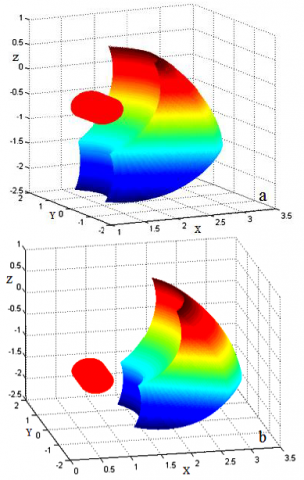
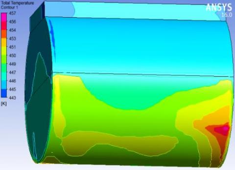
Figure 8. Temperature cloud map
The heating time, heat flux and mixing blade speed were initialized and taken as input parameters. After the calculation, the post-processing interface was entered to obtain the transient simulation results (Figures 7~8).
Figure 7 is a vector diagram of how fast the HMA flows under the action of mixing blades. The mixing attempts to accelerate the HMA flow and ensure uniform heating of the HMA. As shown in Figure 7, the maximum flow speed of the HMA was 1.41m/s. Figure 8 offers a cloud map on the outer surface temperature of the mixer.
4.3 Results analysis
The ranges of the input parameters were configured by the response surface method (Table 5).
Table 5. Ranges of the input parameters
|
Input parameters |
Simulation time/s |
Blade speed/ radian/s |
Heat flux/ W/m2 |
Blade thickness /mm |
|
Initial value |
1800 |
3.1416 |
10000 |
10 |
|
Minimum value |
600 |
2.1416 |
5000 |
20 |
|
Maximum value |
3000 |
4.1416 |
15000 |
30 |
Then, the HMA’s maximum, minimum and mean temperatures were taken as the outputs, and respectively configured by the expressions Maxtemp=maxVal(T)@liao, Mintemp=minVal(T)@liao and wendu=[Maxtemp+Mintemp]/2. On this basis, the author derived how temperature correlates with heat flux and time, and with heat source and blade speed (Figures 9~12).
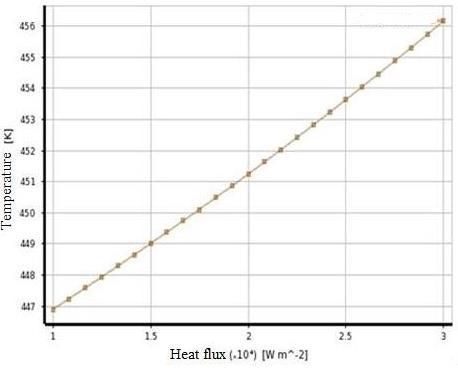
Figure 9 Relationship between heat flux and temperature
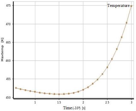
Figure 10. Relationship between time and maximum temperature
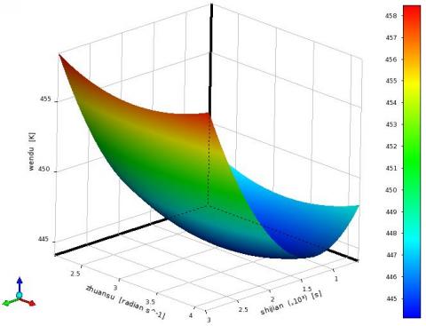
Figure 11. Relationship between temperature, blade speed and time
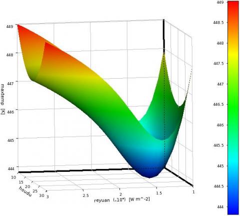
Figure 12. Relationship between maximum temperature, heat flux and blade thickness
As shown in Figure 9, the heat flux is positively correlated with the HMA temperature. Figure 10 indicates that the maximum temperature first slightly dropped from the high initial level and then increased rapidly, under the action of mixing.
The relationship between temperature, blade speed and time in Figure 11 demonstrates the impact of blade speed on temperature. The relationship between maximum temperature, heat flux and blade thickness in Figure 12 manifests the direct and nonnegligible influence of blade thickness on the HMA flow in the mixing process.
Considering the above results of the response surface method, the blade thickness of the designed mixer was set to 10mm, and the heating power of the mixer was set to 13kW (heating power=heat flux×heat source area 1.3m2). Under these parameters, it takes 30min to heat up 70kg HMA to 160 $^{\circ} \mathrm{C}$ , which meets the maintenance requirements.
Figure 13 Overall layout of the road maintenance vehicle
1. The mixing tank 2. The vertical loading mechanism 3. The pulverizing tank 4. One arm 5. Two arm 6. Three-arm hydraulic cylinder 7. Cutting face 8. Milling face 9. Seam filling face 10. The compaction roller 11. Warning light 12. The HMA transmission though 13. The air heating and pressurizing device 14. Control room 15. Hot asphalt box 16. Asphalt tank 17. Generating set 18. Storage bin 19. Hydraulic pump station 20. The waste transmission trough 21. The waste collection hopper 22. The rear HMA discharge trough 23. Hydraulic cylinder 24. Rack and pinion mechanism 25. Fixed-end toothed disc box 26. Rotating end toothed disc box body
The overall layout of our road maintenance vehicle is illustrated in Figure 13. Firstly, the cutting and milling waste is collected manually into the waste collection hopper 21, and then transmitted via the waste transmission trough 20 to the vertical loading mechanism 2. Next, the waste will be pulverized in the pulverizing tank 3, and relocated to the mixing tank 1, where it is mixed with asphalt under heating. The HMA will be transported via the HMA transmission though 12 and the rear HMA discharge trough 22 into the maintenance area. Finally, the HMA will be compacted by the compaction roller 10. In Figure 13, the item marked by 15 is a hot asphalt box that stores and keeps the temperature of hot asphalt. The box can heat up asphalt to a certain temperature. The hot asphalt in 15 can be pumped by the asphalt pump to 1 or poured into the cracks on the road. The air heating and pressurizing device 13 is connected to the high pressure air port on the pouring working face 9. This device cleans and blows dry the cracks with high pressure air. The indexable maintenance equipment has three working faces, which respectively correspond to the left side (pouring working position), lower side (milling working position) and right side (cutting working position). During the operation, the maintenance equipment can switch between the three working positions based on the actual demand.
The proposed indexable maintenance equipment integrates multiple functions, such as milling, cutting and pouring. While the traditional maintenance vehicle carries small milling, cutting and pouring devices, our design offers a unified power source that drives all three devices simultaneously. This design has many advantages over the traditional method: there is no redundant power source, and thus no wasted cost; the integrated equipment is small in size, making it easy to be operated by the manipulator; the labor-intensity of equipment lifting is minimized; the maintenance becomes safer, more convenient and more automated; the workers no longer need to work in a harsh environment.
For the proposed road maintenance vehicle, all the functions were designed to solve the cracks caused by common road diseases and fill up small pits. As a result, our maintenance vehicle can fulfil specific maintenance purposes, despite its small size.
Since the vehicle is normally stationary in the maintenance process, the hydraulic system of our vehicle draws power from the engine via a power-take-off unit. In addition, the onboard generator set was relatively small in power and volume, because it only needs to power the heating and control systems, while most other devices are powered by the hydraulic system. Therefore, our vehicle is more compact and less expensive than traditional road maintenance vehicles.
What is more, our road maintenance vehicle has a highly intelligent and easy-to-use waste collection system to reuse the asphalt waste generated by milling and cutting. Thus, our vehicle is friendly to the environment.
The project supported by Natural Science Basic Research Plan in Shaanxi province of China (Program No. 2019JQ-179).
Scientific research program funded by Shaanxi Provincial Education Department of China (Program No. 19JK0034).
[1] Pantha, B.R., Yatabe, R., Bhandary, N.P. (2010). GIS-based highway maintenance prioritization model: An integrated approach for highway maintenance in Nepal mountains. Journal of Transport Geography, 18(2): 426-433. https://doi.org/10.1016/j.jtrangeo.2009.06.016
[2] Xie, B.L., Li, Y., Jin, L. (2010). Vehicle routing optimization for deicing salt spreading in winter highway maintenance. Procedia-Social and Behavioral Sciences, 21(6): 86-97. https://doi.org/10.1016/j.sbspro.20-13.08.108
[3] Li, X., Zhou, Z., Lv, X. (2017). Temperature segregation of warm mix asphalt pavement: Laboratory and field evaluations. Construction and Building Materials, 136(1): 436-445. https://doi.org/10.1016/j.conbuild-mat.20-16.12.195
[4] Zhang, J., Zhang, W.L., Li, R., Ma, B., Ye, M., Mao, X.S., Zhang, D.P. (2014). Lifter design of multifunctional asphalt pavement road maintenance truck for Qinghai-Tibet Aera. Journal of Guangxi University, 39(2): 287-293.
[5] Wan, Y.P., Song, X.D., Guo, F. (2015). Structural design of road comprehensive maintenance vehicle based on TRIZ theory. Mechanical Design, 32(3): 111-114.
[6] Ma, B., Mao, X.S., Ye, M. (2013). Quick multifunctional maintenance of asphalt pavement in high altitude and low temperature areas: China. Patent Application CN103088746A.
[7] Deng, L., Wang, W., Cai, C.S. (2017). Effect of pavement maintenance cycle on the fatigue reliability of simply-supported steel I-girder bridges under dynamic vehicle loading. Engineering Structures, 133(15): 124-132. https://doi.org/ 10.10-16/j.engstruct.2016.12.022
[8] Wang, S.J., Wang, Z., Yuan, K. (2015). Qinghai-Tibet highway engineering geology in permafrost regions: Review and prospect. China Journal of Highway and Transport, 28(12): 1-8.
[9] Zhang, Y.Z., Du, Y.L., Sun, B.C. (2014). Roadbed deformation of high-speed railway due to freezing-thawing process in seasonally frozen regions. Chinese Journal of Rock Mechanics and Engineering, 12(33): 2546-2553. https://doi.org/10.1372-2/j.cnki.jrme.2014.12.021
[10] Ye, Z.R., Shi, X.M. (2012). Vehicle-based sensor technologies for winter highway operations. IET Intelligent Transport Systems, 6(3): 4336-4345. https://doi.org/10.1049/iet-its.2011.0129
[11] Wu, D.Y., Yuan, C.W. (2016). A life-cycle optimization model using semi-Markov process for highway bridge maintenance. Applied Mathematical Modelling, 43(11): 1-9. https://doi.org/10.1016/j.apm.20-16.10.038
[12] Liu, M. (2005). Bridge annual maintenance prioritization under uncertainty by multiobjective combinatorial optimization. Computer-Aided Civil and Infrastructure Engineering, 20(5): 343-353. https://doi.org/10.1111/j.1467-8667.2005.00401.x
[13] Ye, M., Mao, X.S. (2014). Freeze depth predicting of permafrost subgrade based on moisture and thermal coupling model. KSCE Journal of Civil Engineering, 19(6): 24-32. https://doi.org/10.1007/s12205-014-0685-x
[14] Xiao, Y., Chen, C.S. (2015). Enhanced sunlight-driven photocatalytic activity of graphene oxide/Bi2WO6 nanoplates by silicon modification. Ceramics International, 41(8): 12-20. https://doi.org/10.1016/j.ceram-int.2015.04.103
[15] Dong, C.L., Liu, H.T., Yue, W., Huang, T. (2018). Stiffness modeling and analysis of a novel 5-DOF hybrid robot. Mechanism and Machine Theory, 125(7): 80-93. https://doi.org/10.1016/j.mechmachtheory.2017.12.-009
[16] Yao, X.Y., Ding, H.F., Ge, M.F. (2018). Task-space tracking control of multi-robot systems with disturbances and uncertainties rejection capability. Nonlinear Dynamics, 92(4): 1649-1664. https://doi.org/10.1007/s11071-018-4152-y
[17] Qi, X., Shen, X. (2014). Multidisciplinary design optimization of turbine disks based on ANSYS workbench platforms, Asia-Pacific International Symposium on Aerospace Technology, 99: 1275-1283. https://doi.org/10.10-16/j.proeng.2014.12.659
[18] Zhang, Z.J., Zhou, H.B., Duan, J. (2017). Design and analysis of a high acceleration rotary-linear voice CoilMotor. IEEE Transactions on Magnetics, 53(7): 1-9. https://doi.org/10.1109/TMAG.2017.2675359
[19] Liu, X., Jenkins, C.H. (2001). Large deflection analysis of pneumatic envelopes using a penalty parameter modified material model. Finite Element Analysis and Design, 37(3): 233-251. https://doi.org/10.10-16/s0168-874x(00)00040-8
[20] Luo, Y.J., Xing, J. (2017). Wrinkle-free design of thin membrane structures using stress-based topology optimization. Journal of the Mechanics and Physics of Solids, 102: 277-293. https://doi.org/10.1016/j.jmps.2017.02.003