Nand Kishore Sharma*![]() | Surendra Rahamatkar
| Surendra Rahamatkar![]() | Abhishek Singh Rathore
| Abhishek Singh Rathore![]()
© 2024 The authors. This article is published by IIETA and is licensed under the CC BY 4.0 license (http://creativecommons.org/licenses/by/4.0/).
OPEN ACCESS
In the realm of transport development, the fusion of modern technology and vehicle surveillance in roadside areas becomes indispensable. Traditional surveillance demands continuous monitoring through closed-circuit television cameras. It results in a huge amount of data, which requires high computation. This study delves into the challenges of real-time processing of vehicle surveillance within smart cities with quality data. In addition to a specific focus on monitoring the roadside traffic region despite technological advancements, including target variability, lighting conditions, and occlusion, the manuscript introduces a lightweight contour-based convolutional neural network to address these challenges. The proposed work aims to gain the maximum features from the vehicle via detecting the optimal position and incorporating a Region-Proposal-Network, Region-of-Interest-Align and pooling, Non-Maximum-Suppression, Structural-Similarity-Index, and Peak-Signal-to-Noise-Ratio. The proposed work extracts hierarchical information from a custom video dataset and demonstrates superior performance with an accuracy rate of 97.36% and a minimum loss of 0.0816 in an elapsed time of 1s 159ms. Furthermore, it achieves a validation loss of 0.1506, and a validation accuracy of 96.46%. Additionally, manuscripts illustrate different datasets and models through a systematic literature review. Moreover, the manuscript also illustrates the Smart-City framework and Integrated Traffic Management System architecture.
real-time vehicle surveillance, Smart-City, vehicle makes and model recognition, structural similarity index, scale-invariant feature transform, contour-based CNN, transport development
In the rapidly expanding era of technology, the systematic monitoring of individuals has become pervasive. In smart cities, the demand for surveillance extends to roadside traffic areas, where video surveillance systems are instrumental in analyzing traffic flow, detecting incidents, and enforcing traffic laws [1]. The roadside surveillance encompasses intricate trending technologies, good-quality and meaningful data sources with reliable communication protocols. However, the implementation of such type of complex setup and their regular maintenance incurs a considerable cost. This cost may occur just because of complex software, highly configured hardware, and high computation resources. Therefore, striking a balance between the advantages and drawbacks of complex surveillance systems becomes imperative in addressing the multifaceted challenges those are associated with them.
To collect the data from different road-side traffic areas the wireless-sensor network [2, 3] has appeared as the most capable technology. In addition, computer vision also plays a very crucial role in numerous surveillance applications. It is found capable of handling challenges like real-time computation amidst many vehicles at peak traffic times and occlusions [4].
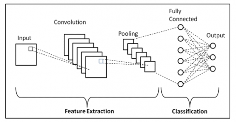
In recent years, the deep-learning techniques have been harnessed during vehicle surveillance because of their good performance and features. Its adoption is substantiated due to its gainful attributes, robustness, generalization, and scalability. For the same, the Deep Learning Convolutional-Neural-Network (CNN) comprises two core components namely feature extraction and classification. Feature extraction is aimed at the acquisition of relevant features in the input data, while classification is responsible for labeling the input data based on the ascertained characteristics. This architectural configuration is illustrated in Figure 1.
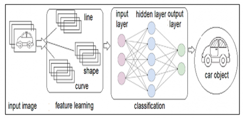
The feature extractor component typically includes multiple convolutional layers, each designed to learn fundamental features such as edges and corners, which represent low-level features in the context of the data analysis process. These low-level features are then amalgamated and processed by subsequent layers to learn higher-level features such as shapes. The classifier encompasses a fully connected layer, which takes the extracted features as an input and a probability distribution over the possible vehicle classes as an output. Figure 2 depicts the working of CNN to detect the vehicle.
Figure 1. Convolutional neural network architecture
Figure 2. Working with CNN to detect vehicle and feature extraction
1.1 Smart city framework for transport development and integration
The concept of a smart city represents an advanced urban environment built on robust data infrastructure and sophisticated frameworks, specifically tailored for the development and integration of transportation systems. The foundational elements of the smart city framework include physical infrastructures, networking systems, central computing centers, and data storage systems. All elements are essential in the context of smart transport management, as illustrated in Figure 3 [5].
Figure 3. The general smart city framework
At the core of this architecture lies the physical infrastructure, strategically planned with sensors, devices, and cameras. These devices are aimed at capturing and generating transportation-related data. This raw data is then transmitted through network communication mediums to a central computation center, where it undergoes processing to extract pertinent details, such as vehicle information during Red-Light-Violation incidents at roadside zebra crossings.
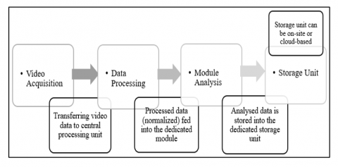
The seamless exchange of data between acquisition devices and central computing centers is facilitated through various communication channels and mediums. The processed data then traverses through these communication mediums to reach virtual machines, cloud computing devices, and servers within the central computing center before being stored. The exchange of information is essential; however, the emphasis is on confirming the reliability of the data [6]. Reliable information is indispensable for making swift decisions and generating timely responses within the framework of a smart city. The applications within smart cities utilize gathered data to forecast outcomes, which depend significantly on a well-designed network and astute management systems [7]. The effectiveness solely relies on a well-designed network and an ITMS. They both are essential for the overall functioning of the smart city framework. Roadside traffic surveillance takes center stage in smart cities as an integral part of an ITMS. Video streams act as the predominant medium in surveillance with video analytics. Figure 4 depicts a comprehensive workflow of a modern surveillance system, outlining the intricacies of surveillance within a smart city.
Figure 4. A comprehensive workflow of the modern video surveillance system
The surveillance process initiates with video acquisition, where cameras and sensors are strategically deployed as acquisition devices. The acquired video data is then transmitted to a central processing unit for further analysis, where raw video streams are transformed into digital formats to enable efficient processing and storage. In the module analysis stage, the processed data is fed into dedicated software modules for object detection by employing deep-learning models for accurate results. Following data processing and analysis, the information is stored in a dedicated unit. These units are either on-site or cloud-based, catering specifically to the surveillance of roadside traffic and incorporating ITMS.
1.2 Integrated-traffic-management-systems (ITMS)
The ITMS is illustrated by a conjunction of technologies, data inputs, and communication protocols. They are aimed at enhancing the integration of modern transport development. The deployment of such a system demands meticulous planning of acquisition devices and equipment. The intention behind this plan is to consider a coverage area, camera angles, and lighting conditions. The system incorporates two distinct camera types: the Automatic Number Plate Recognition (ANPR) camera and the Red-Light Violation Detection (RLVD) camera, each serving a specific role as illustrated in Figure 5. This setup is implemented across the city and establishes a strong interconnected network for efficient transmission in capturing real-time information for transport management and integration. This setup is aimed to optimize the detection and tracking of vehicles during their stationary periods, emphasizing safety and security.
The architectural configuration illustrated in Figure 6 and Table 1 provides a comprehensive overview of the smart city ITMS architecture.
Figure 5. Camera set-up of ITMS at road-side traffic area
Figure 6. ITMS architecture in Smart-City
These acquisition devices in the combination of RLVD and ANPR are situated approximately 20 feet (6.5 meters) above the road and 13 meters from the zebra crossline, the cameras possess a focal length of 3.2-3.5 meters, strategically focused on the zebra crossline. The ANPR camera is committed to detecting the vehicle's number plate and capturing a single image, while the RLVD camera functions as a surveillance camera, capturing four additional images upon detecting a violation. The captured data is transformed through a media converter and is transmitted back to the Local Processing Unit (LPU) via fiber optic cables. The interconnection of devices is facilitated through an L-2 switch employing cat-6 cables. Subsequently, the LPU transmits this processed data to the control room via fiber optic cables, where further processing occurs. The control room is equipped with an L-3 switch, a storage unit, and a set of 3-4 servers, including the Central Server, Data Server, and Media Server. The Central Server, serving as the master server, issues instructions to the other servers, while the Media Server functions as an aggregation point for data from various junctions. It operates as a distributed system to reduce server load. Moreover, the data are stored here in multiple replicas to ensure reliability. So that if one server goes down or is manipulated during a cyberattack, the same data can be retrieved from another server.
Table 1. Elements and their uses within an ITMS architecture in Smart-City
|
Key Elements & Uses |
Description |
|
Cameras: Data collections |
Cameras with high resolution, such as Pan-Tilt-Zoom (PTZ) cameras, are strategically installed based on specific needs to capture live footage of traffic. |
|
Video Analytics: Data processing and analysis |
This software utilizes sophisticated algorithms to analyze the data, identify and assess vehicles, recognize license plates, and detect incidents. |
|
Servers: Data storage |
The video data that has undergone processing, along with the analytics data, is stored either on local servers or in the cloud for subsequent processing. |
|
Communication network: Communication infrastructure |
A dependable communication network is crucial for the transmission of video and data among cameras, analytics software, storage systems, and end-users. |
|
User interfaces and applications |
An interface that is easy for users to navigate enables the supervision and management of the system through analyzed data and reports. |
|
Decision support and control systems: Integration with other systems |
Based on the analyzed data and processing outcomes, decision support systems provide suggestions to traffic management authorities and control systems. Video surveillance of roadside traffic, such as integrated traffic management systems, can be integrated with additional traffic signal control systems and emergency response systems [8]. |
This manuscript focuses on a cost-efficient model for extracting low-level vehicle features for efficient roadside traffic surveillance. That can be achieved with the combination of the Integrated Traffic Management System (ITMS) with Smart-City transport development. The proposed work employs a lightweight contour-based CNN to extract hierarchical information from the vehicle by employing a custom video dataset while considering real-world scenarios. The key contributions of this work include two phases:
(1) Transforming the acquired vehicle video into separate frames.
(2) Selecting the best vehicle position frame to maximize feature extraction.
The proposed work incorporated a Region Proposal Network (RPN), Region of Interest Pooling or Region of Interest Align, and Non-Maximum Suppression to optimize the entire detection process. Apart from this, the feature extraction is enhanced through the utilization of the Structural-Similarity-Index (SSIM) with thorough parameters calculation, including Mean Luminance Similarity (MLS), Mean Contrast Similarity (MCS), Mean Structure Similarity (MSS), and Peak-Signal-to-Noise-Ratio (PSNR) for each duo frame.
The use of contour-based detection algorithms in the proposed methodology is justifiable for several reasons, despite the availability of state-of-the-art. The choice of the proposed approach aligns with the specific objectives, dataset characteristics, and real-world traffic surveillance challenges like varying lighting conditions, complex scenes, and occlusions. Contour-based detection algorithms are inherently versatile for handling complex scenarios. Unlike some algorithms that rely on predefined patterns or features, contour-based methods are adaptive and can identify object edges even in challenging situations.
Overall, this research contributes to the improvement of robust surveillance solutions tailored for smart city transport, thereby enhancing shelter and efficiency in urban transport systems.
In the context of transport development and integration, vehicle surveillance along the roadside has gained increasing prominence in recent times. The identification of vehicles has emerged as a substantial focus of research due to its diverse and valuable applications, spanning from assisting traffic planners to facilitating real-time traffic management. This literature review encompasses pertinent research within this domain, placing particular emphasis on the comparison of various surveillance techniques and technologies.
Currently, the detection of vehicle objects based on visual information is categorized into [9, 10]: state-of-the-art machine learning and advanced deep learning algorithms. After detection, the recognition of vehicles became an emerging technology that has found widespread applications in ITMS [11]. The fine-grained-recognition and coarse-grained recognition [12] are generally the main categories of vehicle recognition. Fine-grained-recognition presents a confronting due to the subtle differences within the same vehicle class and the high similarity between different vehicle classes. Coarse-grained recognition focuses on dividing vehicles into cars, vans, buses, and truck types. However, the main challenges are inter-class and intra-class diversity. Various approaches have been proposed that utilize local features like Scale-Invariant-Feature-Transform (SIFT) [12, 13], and Speeded-Up-Robust-Features (SURF) [14-16], along with different encoding algorithms, to construct feature dictionaries for vehicle recognition. However, these methods exhibit limitations in accurately discerning specific vehicle attributes. To address these challenges, a novel technique for vehicle classification has been discussed in the study [17].
Various deep-learning algorithms have been applied to video surveillance in recent times, exhibiting diverse levels of accuracy and inherent limitations. The subsequent Table 2 outlines the recent deep learning model employed in video surveillance, accompanied by performance and associated limitations.
Table 2. Comparative overview of various deep learning models
|
Model |
Descriptions |
|
You-Only-Look-Once (YOLO) [18-27] |
It is a widely used object detection model for vehicle surveillance, renowned for its speed and accuracy. It has achieved state-of-the-art performance on benchmark datasets including the COCO dataset. |
|
Faster R-CNN [28-33] |
It is a prevalent object detection algorithm employed during vehicle surveillance. It operates in two stages, generating region proposals and then classifying objects within those regions. The performance is good but may be slower than YOLO. |
|
Single-Shot-Multi-Box-Detector (SSD) [34-37] |
It is a high-speed and accurate real-time object-detection technique, excelling on the COCO dataset and various other benchmark datasets. |
|
Mask R-CNN [38] |
It is an advanced version of Faster R-CNN and identifies instances as well as objects. It is an object identification and segmentation method, demonstrating proficiency in recognizing and segmenting objects in video sequences. |
|
Panoptic Feature Pyramid Networks (PANet) [39] |
It is an extension of Mask R-CNN, and introduces a spatial consideration mechanism and a feature pyramid attention (FPA) module, enhancing performance in instance and semantic segmentation tasks. |
|
PointRend [40] |
It is an extension of Mask R-CNN and employs a pixel-level rendering approach for image segmentation. It utilizes a point-based sampling technique and a learnable interpolation module, producing high-quality instance segmentation results. |
|
EfficientDet [41, 42] |
It is a modern object detection technique. It is known for good performance and quick response through neural architecture search and efficient scaling. It shows promise in enhancing surveillance systems but demands substantial processing resources. |
|
CenterNet [43] |
It is a contemporary object recognition technique predicting object centers and offsets using a single heatmap. It requires a larger training dataset. Demonstrates good performance but may face challenges in detecting small objects. |
|
DeepSORT [43] |
It is a contemporary object-tracking methodology, that exhibits high tracking accuracy on benchmarks like MOTChallenge, MOT17, and DukeMTMC. It may face challenges with occlusions, necessitating additional post-processing approaches to enhance tracking effectiveness. |
The algorithm functions by analyzing vehicles and discerning essential features. Various algorithms are available for extracting features of four-wheeler vehicles for surveillance, contingent on the surveillance system type and available data. Several common algorithms include the License Plate Recognition (LPR) Algorithm [44-47] employs image processing techniques to detect and recognize the license plates of four-wheeler vehicles. Subsequently, it utilized methods like binarization, edge detection, and character segmentation to extract characters from the license plate. Object Detection and Tracking Algorithms [28, 35, 48-54] identified the presence of four-wheeler vehicles within a given scene. Techniques like Haar Cascades, Histogram-of-Oriented-Gradients (HOG), and CNN are applied to recognize vehicles in the image.
The Vehicle Make and Model Recognition algorithm [55] analyses visual attributes of the car, such as shape, and size, utilizing deep learning algorithms to classify the vehicle under a specific brand and model for Intelligent Transportation Systems (ITSs) [6]. By incorporating deep learning techniques a robust real-time system achieves high accuracy. The real-time approach combines the SURF detector with the Support Vector Machines (SVM) and provides a solution for Make and Model Recognition (MMR) to recognize car types from single images based on the geometry and appearance of car emblems in rear-view images. These images are captured by traffic cameras. The aim is to learn both the geometry and appearance of car emblems for accurate vehicle model recognition. The SURF features of vehicles' front- or rear-facing images are extracted and stored as codewords in dictionaries. Addressing the intricacies of vehicle model recognition, the research [15, 56, 57] introduced a real-time vehicle make and model recognition (VMMR) using a Bag-of-Speeded-Up-Robust-Features (BoSURF).
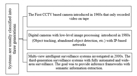
According to the survey, video surveillance systems have advanced over three generations, as illustrated in Figure 7.
Figure 7. Generations of surveillance system
The literature review underscores the versatility of deep learning, offering solutions across diverse domains and complex problem scenarios. The identified research gaps are listed in Table 3.
In summary, this comprehensive literature review delves into the latest research in this field, focusing on diverse surveillance methods and technologies. The collective findings emphasize that different deep learning models exhibit varying performance for different tasks during vehicle video surveillance such as detection, tracking, and classification, normally it ranges from 90-95%. Consequently, selecting a deep learning model for a specific application should be guided by the task requirements, computational resources, and dataset characteristics.
Moreover, Deep learning also plays a crucial role in vehicle surveillance and provides an automated and hierarchical approach to extracting valuable insights from vehicle images or video frames. Algorithms such as License Plate Recognition (LPR), Object Detection and Tracking, and Vehicle Make and Model Recognition are used for feature extraction..
Table 3. Potential research gaps identified from systematic literature review
|
Parameter |
Descriptions |
|
Unnecessary data |
Developing effective techniques to handle imbalanced data for vehicle recognition, ensuring unbiased model training. |
|
Real-time computation |
Probing methods to enhance the real-time processing capabilities of deep learning algorithms, especially in resource-constrained environments. |
|
Integration of the latest models |
Exploring strategies to seamlessly integrate modern techniques like EfficientDet, CenterNet, and DeepSORT into existing surveillance systems for enhanced functionality. |
|
Optimization of computational resources |
Developing algorithms that optimize computational resources, ensuring efficient processing on low-power devices without compromising accuracy. |
|
Incorporation of multiple procedures |
Integration of various algorithms, including LPR, Object Detection, and VMMR to enhance the overall efficiency and accuracy of vehicle surveillance. |
|
Adaptation to circumstances |
Capable algorithms for adapting a diverse environmental condition, such as varying lighting, weather, and occlusions, to ensure consistent and reliable vehicle recognition in all situations. |
|
Improved image pre-processing techniques |
Finding advanced image preprocessing techniques to enhance image quality, reduce noise, and improve the clarity of captured vehicle images, aiding in more accurate recognition processes. |
Over the preceding decades, a multitude of datasets have been extensively employed in the domain of object detection and vehicular surveillance, as comprehensively elucidated in the literature review undertaken within this research manuscript. The ensuing Table 4 provides prevalent datasets employed in the realm of vehicle detection and video surveillance, accompanied by descriptive details and rationale for their utilization.
The custom dataset excels in aligning with specific research goals for vehicle detection in realistic traffic scenarios. It offers diversity, real-world legitimacy, and a deliberate focus on the research objectives. Real-world challenges, such as partial occlusions, enhance the dataset's complexity, addressing unique hurdles during vehicle analysis. While benchmark datasets may not precisely match the targeted research focus on optimal vehicle position detection. The custom dataset stands out for its alignment with specific research goals with the ability to capture vehicles from multiple angles conducive to comprehensive vehicle analysis.
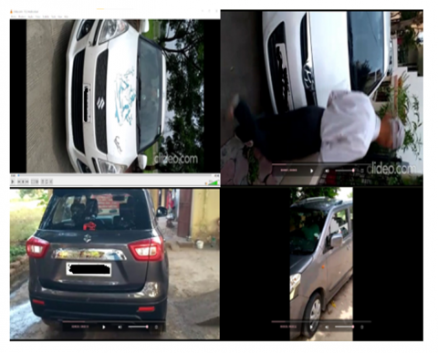
The experimental dataset in this study is meticulously curated to meet the evolving needs of integration of transport development. The target location is the roadside traffic signal area, here vehicles temporarily halt according to signal time. Typically, the signal time ranged from 30 seconds to 2 minutes, hence accordingly videos were recorded. This bespoke dataset features 20 video recordings 5 for each Indian four-wheeler vehicle, the duration of the video ranges from 50 seconds to 1.5 minutes. Each video contains 300 frames. Notably, the videos include four distinct vehicle brands: Hyundai i20, Maruti-WagonR, Maruti-Swift, and Maruti-Suzuki-Brezza, selected to accommodate variations in body length and style. All decided vehicles exhibit different colors. The reason for selecting different vehicles was to account for variations in body length and style across different models, which surely prevented the model from being biased during training.
The videos were captured in the morning, afternoon, and evening, with a moving camera. The videos were strategically recorded from diverse angles (+15 to -15 degrees relative to the scene) to ensure coverage of vehicles from various positions and viewpoints. This approach facilitates the identification of optimal vehicle positions. The videos also consider different meteorological conditions, including sunny and opaque scenarios, with some recordings featuring partial occlusions caused by shadows from trees and individuals. Sample video snippets of the recorded dataset are illustrated in Figure 8.
This comprehensive and diverse custom dataset serves as a valuable resource for training and testing vehicle detection, providing real-world challenges and scenarios that extend beyond the limitations of existing benchmark datasets.
Table 4. Commonly used datasets in vehicle detection
|
Dataset |
Description |
Justification |
|
KITTI [58-60] |
It is a large size dataset, containing real-world data annotated 2D and 3D object labels. Data is accumulated from cars driving around the city which comprises various cameras and sensors. The dataset comprises 323 annotated images categorized into the road, vertical, and sky classes, 252 acquisitions with RGB and Velodyne scans, divided into 140 for training and 112 for testing. Additionally, there are 170 training images and 46 testing images, covering 11 classes. |
The benchmark dataset is for autonomous driving research. It proposes real-world scenarios but may lack diversity in vehicle models and colors. |
|
CamVid [61, 62] |
It is a moderate-size street scene video dataset annotated with object segmentation and classification. It is five video sequences captured by a 960×720 resolution camera, annotated in various 32 classes. |
Appropriate for vehicle detection in urban contexts nevertheless may not cover diverse vehicle types. |
|
City-Scapes [63] |
It is a large dataset, that recorded urban street scenes in various cities. Data is annotated for semantic segmentation and object detection. It contains approx 5000 fine annotated and 20,000 coarse annotated images. |
Primarily used for semantic segmentation-related tasks and may be employed for vehicle detection in urban environments. |
|
MIO-TCD [64] |
It is a large-size traffic camera images and video dataset that covers various traffic scenarios and vehicle categories. It consists of a localization dataset of 1,37,743 full video frames with bounding boxes around traffic objects and a classification dataset of 6,48,959 crops of traffic objects from the 11 classes. |
Offers diversity but may be deficient in comprehensive annotations for several tasks. |
|
COCO [65] |
It is a very large size and large-scale dataset with a diverse collection of images with object annotations in various contexts. The dataset consists of 328K images of 80 object categories. |
It is a comprehensive dataset for object detection. Its diverse context may not align precisely with the study's objective. |
|
MOT-Challenge [66] |
It is a moderate to large-size dataset with multiple camera views and annotated object tracks. Focuses on multi-object tracking tasks |
Predominantly adapted for tracking tasks and may require adaptation for single-frame object detection scenarios. |
Figure 8. Recorded video snippets featuring various Indian vehicles captured at different times and under diverse occlusion conditions
This section depicts the entire proposed methodology and implementation details.
4.1 Proposed methodology
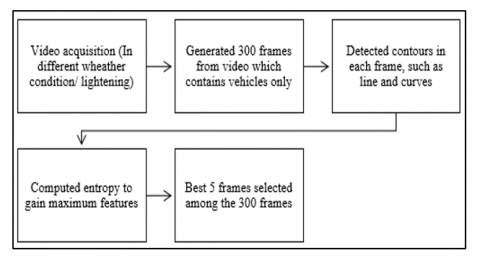
The contour-based detection approach commonly utilizes edge detection. The graphical representation of the proposed approach is illustrated in Figure 9.
Figure 9. Graphical representation of the proposed approach
Initially, the video acquisition camera will record the video. This recorded video will be used as an input. The proposed work will process the video and generate 300 frames, which comprises vehicles only. For the same, the contours will be detected, and the contour feature will be computed (as illustrated in the algorithm: contour-based detection) in each frame to resemble the vehicle only.
In state-of-the-art, the contour-detection approach uses edge detection to identify and detect the contours. This approach finds the boundaries between regions of the image with different intensity values and gradients. In vehicle detection to get the optimal position of the four-wheeler, these boundaries can be understood as the outer hood or bonnet, bumper, bumper grill, side mirrors, side indicators, front glass, license plate, vehicle logo, headlights, etc. It means, the frames which contain maximum contours, have maximum features.
Therefore, the optimal position of the vehicle is one where maximum features are present. Once the contours have been identified, they can be used to extract features from the frame. Later, all processing will performed on these frames only. Further processing includes the computation of SSIM with parameters and in-depth analysis of the vehicle through pixel intensity and distribution.
Therefore, these methods involve identifying the boundaries between areas of the image with different intensity values or gradients. The entire suggested methodology is segmented into two phases:
Phase-I: Transforming video into individual frames for vehicle detection
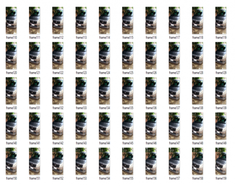
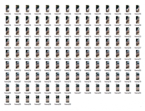
The proposed workflow is initiated by systematically processing a sequence of continuous video frames, ensuring the careful conversion of each frame into an image representation, and storing it in the 'frameimages' list. This methodical approach guarantees the seamless capture of every frame, laying the foundation for in-depth analysis. Some of the sample frames are depicted in Figures 10, 11, and 12. Selected 50 frames of Figure 10 represent the front view of the vehicle, selected 50 frames of Figure 11 represent the partial side view of the vehicle, and selected 119 frames of Figure 12 represent the total side view of the vehicle.
To give in-depth clarity to video frames of the front view, partial side view, and total side view, a single sample frame is picked from Figures 10, 11, and 12, which is illustrated in Figure 13.
Figure 10. Sample 50 frames depicting the front view of the vehicle
Figure 11. Sample 50 frames depicting the partial side view of the vehicle
Figure 12. Sample frames depicting the complete side view of the vehicle
Figure 13. Sample frame from each view of the vehicle
Contour-based vehicle object detection in a video involves detecting the contours of vehicles in each frame of the video and tracking them across frames to determine their motion and trajectory. The set of all contours can be represented through Eq. (1):
Contours = {Ctr1, Ctr2, Ctr3, ..., Ctrn} (1)
In the above Eq. (1) Contours represent the set of contours in the image, and Ctr1, Ctr2, Ctr3, ..., Ctrn represents individual contours within the set. Each contour can be represented as a set of points or a continuous curve that defines the boundary of an object in the image, these boundaries can be understood as the outer hood or bonnet, bumper, bumper grill, side mirrors, side indicators, front glass, license plate, vehicle logo, headlights, etc. Let V_Objt be the set of vehicle objects in frame t, and Contourst be the set of contours detected in frame t. The contour-based vehicle object detection can be defined via Eqs. (2), (3) and (4):
Contourst = Detect_Contours (frame t) (2)
V_Objt = {Ctri|Ctri∈Contourst, Is_VehicleContour(Ctri)} (3)
V_Objt = Track_Vehicles(V_Objt -1, V_Objt) (4)
The Eqs. (2)-(4) parameters are as follows:
The algorithm detects and identifies the contours in each video frame that correspond to vehicles. This progression is repetitive for each video frame.
|
Algorithm - contour-based-detection Inputs: VideoStream Outputs: V_Obj = {v1, v2, ..., vn} C(t) = {c1, c2, ..., cm} f(ci) = {f1, f2, ..., fk} Procedure: Initial set of vehicle objects V_Obj = {} for each_frame t in the video: a. Extract contours C(t) in the video frame b. for each_contour c in C(t):
c. Track the motion and trajectory of each vehicle object in V_Obj over time. End |
In the proposed algorithm, the Outputs the V_Obj represents the set of vehicle objects, C(t) represents the set of contours in frame t, ci represents the ith the contour in C(t), f(ci) represents the feature vector for contour ci, and k represents the number of contour features.
Utilizing contour detection techniques, the proposed method adeptly identifies vehicle contours within a predefined detection area. The process meticulously employs filters with specific location and size criteria, ensuring that only relevant contours are retained for closer examination. To improve result visualization, the pipeline enhances its functionality by visually overlaying the identified vehicle outlines onto the original video frames, providing a clear representation of the outcomes.
In-depth calculations for the same will be conducted in phase-II.
Phase-II: Identifying and choosing the best vehicle position to maximize feature extraction
In addition to vehicle detection, the objective is to determine the ideal positioning of vehicles. From the multitude of frames produced by the above algorithm (comprising 300 frames exclusively showcasing vehicles), the identification of the top frames (5 frames) relies on the presence of the highest number of features. The author employed a methodology based on features to extract specific attributes or characteristics of vehicles, which were then utilized to train the model in identifying vehicles in the optimal position with the greatest number of features. Therefore, a crucial element of this process involves selecting the most informative features for the given task.
In computer vision, feature gain denotes the amount of information acquired by extracting a particular feature from an image or object. Maximum feature gain is attained when the feature can effectively distinguish the object of interest from other objects in the image. The calculation of maximum features is determined through Eq. (5):
G(DataSet, Features)= H(DataSet)-H(DataSet $\mid$ Features) (5)
In the Eq. (5), the parameters denote:
Let, DataSet be D and Features is F, then the maximum feature gain represents the amount of information gained by adding feature F to the dataset D. The entropy of the dataset D represents the amount of uncertainty in the dataset, while the conditional entropy of the dataset given feature F represents the amount of uncertainty in the dataset that can be explained by feature F. The mathematical expression for maximum feature gain from a vehicle object can be represented as follows:
Let V_Obj be the set of vehicle objects in an image, and F be the set of features that can be extracted from each object. The maximum feature gain can be defined via Eq. (6):
$\max (F i)=\operatorname{argmax} F(u, v) * \log \left(\frac{P\left(V_{O b j} \mid u, v\right)}{P(! V \mid \text { obj|u,v) }}\right)$ (6)
In Eq. (6), the parameters denote:
It is based on the principle of information gain to measure the uncertainty while extracting a particular feature. The feature that maximizes this reduction in uncertainty is considered the feature that provides the most information about the presence or absence of a vehicle object in the image.
To extract feature maps of a consistent size from the image's feature map, Region-of-Interest-Pooling (RoI pooling) or Region-of-Interest-Align (RoI align) techniques are employed. In RoI pooling, the RoI is divided into a fixed grid, and max pooling is performed within each grid cell to obtain feature maps of a fixed size. On the other hand, RoI align uses bilinear interpolation to align the RoI to a fixed size, ensuring more accurate spatial alignment. The resulting RoI feature maps are then utilized for localization. Non-maximum suppression (NMS) is applied to eliminate redundant detections and keep only the most confident ones. TensorFlow provides functions, such as tf.image.non_max_suppression, to perform NMS efficiently.
4.2 Implementation
Python 3.8 was chosen for implementing the algorithms discussed in this manuscript, leveraging its open-source nature. Python's extensive collection of robust libraries and packages makes it well-suited for the execution of deep learning models. The implementation occurred on an Intel Core i7 processor with 8 GB of RAM.
The CNN model, constructed using the Keras library, encompasses multiple layers, including convolutional layers with ReLU activation functions, max-pooling layers, dropout regularization (0.25), and fully connected layers. Tailored for vehicle feature extraction and generating a SoftMax output, the CNN model undergoes training with the Adam optimizer and categorical cross-entropy loss function.
Accuracy is monitored as a training metric over 10 epochs with a batch size of 10. The model incorporates processes like frame differencing, contour detection, and classification. Notably, the code allows users to specify a video file for processing. Table 5 provides a summary of the model architecture, detailing layer types, output shapes, and parameters, where out of a total of 2,00,174 parameters, 2,00,168 are trainable, and 6 are non-trainable.
Table 5. The architecture of the proposed CNN with parameters
|
Layer (Type) |
Output Shape |
Parameter |
|
batch_normalization (BatchNormalizaton) |
(None, 28, 28, 3) |
12 |
|
conv2d (Conv2D) |
(None, 26, 26, 32) |
896 |
|
max_pooling2d (MaxPooling2D) |
(None, 13, 13, 32) |
0 |
|
conv2d_1 (Conv2D) |
(None, 13, 13, 64) |
32832 |
|
max_pooling2d_1 (MaxPooling2D) |
(None, 6, 6, 64) |
0 |
|
conv2d_2 (Conv2D) |
(None, 6, 6, 128) |
73856 |
|
max_pooling2d_2 (MaxPooling2D) |
(None, 3, 3, 128) |
0 |
|
dropout (Dropout) |
(None, 3, 3, 128) |
0 |
|
flatten (Flatten) |
(None, 1152) |
0 |
|
dense (Dense) |
(None, 128) |
147584 |
|
dense_1 (Dense) |
(None, 64) |
8256 |
|
dense_2 (Dense) |
(None, 32) |
2080 |
|
dense_3 (Dense) |
(None, 2) |
66 |
5.1 Result
The proposed workflow is initiated by systematically processing a sequence of continuous video frames, ensuring the careful conversion of each frame into an image representation, and storing it in the 'frameimages' list. This methodical approach guarantees the seamless capture of every frame, laying the foundation for our in-depth analysis. To emphasize specific features within these frames, this manuscript explores various plot patterns. Notably, one of the simplest yet most insightful ways to visualize these features is by presenting the image itself. As illustrated in Figures 10, 11, and 12 the author adopts this approach to showcase the series of consecutive video frames as individual images, with each frame treated as an element in the 'frameimages' list.
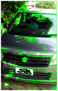
Figure 13 illustrates the front, partial side, and total side view of the vehicle. In the continuation, Figure 14 illustrates all detected contours in the initial and final frames of the video for reference. Here, the dark-colored vehicle is parked in the shadow of a tree, which can be seen in Figure 14.
All detected contours are represented in green to show the different intensity values and gradients. In the first image, the contours are detected on the front glass, bonnet, bumper grill, license plate, and logo. In the second image, the contours are detected on the side glass and gate. Which reflects the maximum contours available in the first image. Therefore, the best vehicle position is illustrated in Figure 15.
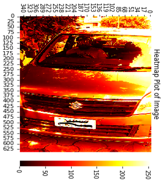
To highlight the maximum information those are detected by the contours illustrated by the heatmap. Figure 16 displays the magnitude of the phenomenon in a 2-dimensional Heatmap.
In addition, Figure 17 depicts the contours of the white Maruti Swift, which has been parked on sunny times without any shade.
Figure 14. Contours detected in the front and side perspectives of an image featuring a Maruti WagonR, taken under the shadow of a tree
Figure 15. Optimal vehicle position, which has maximum features
Figure 16. Heatmap to display the magnitude of the phenomenon in 2-dimensional Heatmap
Figure 17. Detected contours in the frontal view of a White Maruti Swift Vehicle
In Figure 17, all contours are detected on the headlight, bonnet, license plate, grill, and logo. Moreover, the contours are also highlighting the image that is present on the bonnet. All this information may be beneficial for effective surveillance and maximum information gain.
Additionally, the histogram plot can shed light on how the pixel values in an image are distributed. Video histogram analysis focuses on the quantitative analysis and visualization of pixel intensity distributions within images and video frames. The analysis can provide details regarding the brightness, contrast, and pixel intensity as a whole. A histogram is generated using the flattened pixel intensity values. It is divided into 256 bins, representing the full range of pixel intensities (0 to 255). The following is a representation of the histogram plot used for illustrating the distribution of features:
Assume that X = {x1, x2, ..., xn}T is a collection of n observations of a particular feature. The feature values xi can be discrete or continuous. Let B = [B1, B2, ..., Bk] be the collection of k non-overlapping bins. Each of [Bj] symbolizes a range of feature values. The observations in each bin are then counted in the next step.
Let C = "c1, c2, ..., cn" be the collection of counts, with cj denoting the number of observations that fit into the bin Bj. To determine the relative frequencies in each bin, the counts must be normalized in the last step. By dividing each count cj by the sum of the observations n and the width of the bin Bj, this is often accomplished.
Corresponding to the range and distribution of the feature values, each bin can be either uniform or varied. These are possible representations for the normalized counts or relative frequencies as shown in Eq. (7):
$f j=\frac{c i}{(n * B j)}$ (7)
Here, in Eq. (7) the fj stands for the relative frequency of observations in the bin Bj.
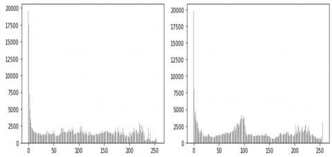
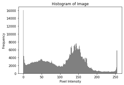
The relative frequencies fj can be plotted against the bin centers or boundaries to get the histogram. Depending on the desired level of granularity in the plot, the midpoints or ends of the bins can be chosen as the bin centers or limits. The resulting plot shows the distribution of the feature values graphically and can be used to spot trends or abnormalities in the data. Figure 18 portrays the pixel distribution of 2 different frames of video first and last frame sequentially, whereas Figure 19 illustrates the intensity of pixels in the video.
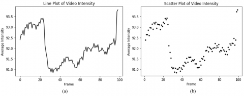
This manuscript also acknowledges the inevitable diversity in pixel intensities across the extracted frames. To examine the relationship between pixel intensity fluctuations and the corresponding video content, it becomes essential to calculate the average intensity across all frames, effectively representing the mean video intensity. Hence, subgraphs (a) and (b) of Figure 20 depict the average intensity of 100 frames through a line plot (showing frame-time correlation) and a scatter plot (facilitating the comparison of pixel intensities) for video analytics.
Figure 18. Histogram of pixel distribution
Figure 19. Pixel intensity in video
Figure 20. (a) Line plot and (b) Scatter plot for visualizing video intensity across 100 frames to observe the correlation between pixel intensity changes and corresponding video
In the realm of practical real-life scenarios, the two different vehicles can look the same or the same vehicle can look different in different positions, illumination, and light intensity. Therefore, metrics that replicate this behavior tend to be more effective. The Structural Similarity Index (SSIM) [67] and Scale-Invariant Feature Transform (SIFT) are two methodologies for extracting features to compare between two images. SSIM serves as a metric to evaluate the similarity between two images. The SSIM computed via Eq. (8) and its parameter descriptions are listed in Table 6.
$\begin{aligned} & \operatorname{SSIM}(I 1, I 2) =\frac{((2 * \mu I 2 * \mu I 2+\text { Const } 1) *(2 \sigma I 1 I 2+\text { Const } 2))}{\left(\left(\mu I 1^2+\mu I 2^2+\text { Const } 1\right) *\left(\sigma I 1^2+\sigma I 2^2+\text { Const } 2\right)\right)}\end{aligned}$ (8)
Table 6. Description of Eq. (8) parameters
|
Parameters |
Description |
|
μI1, μI2 |
Mean: over a window in Image I1 and I2 |
|
σI1, σI2 |
Std deviation: over a window in Image I1 and I2 |
|
σI1I2 |
Co-variance: over a window among Image I1 and I2 |
|
Const1, Const2, Const3 |
Constants |
Table 7 displays Mean SSIM (MSSIM) and Table 8 displays various parameters of SSIM including Mean Luminance Similarity (MLS), Mean Contrast Similarity (MCS), Mean Structure Similarity (MSS), and Peak-Signal-to-Noise-Ratio (PSNR) for pairs of frames (from frame 0 to 299). However, considering the overall similarity of nearly consecutive frames, only 15 comparisons were conducted between the initial and final frames, gradually transitioning between them to compute all parameters. The value ranges from -1 to +1, where +1 signifies identical or extremely similar images, and -1 indicates highly divergent images.
In Table 7, the Frame Image pair column contains frame combinations 0 and 298 i.e. first and almost the last frame. As we move from the first frame to the last frame, similar frames start coming closer. As a result, it can be understood that those frames are identical. Therefore, it can be seen in the table that the value of SSIM for frames 0-298 is small while for frames 14-284 it is large. Therefore, if we continue increasing like this, we will get a large value for the same frame, which will show their similarity.
Table 7. Mean structural similarity index (MSSIM)
|
Frame Image Pair |
MSSIM of Each Pixel SSIM Map |
|
0-298 |
0.17571 |
|
1-297 |
0.17214 |
|
2-296 |
0.16710 |
|
3-295 |
0.16790 |
|
4-294 |
0.16827 |
|
5-293 |
0.17451 |
|
6-292 |
0.18944 |
|
7-291 |
0.19132 |
|
8-290 |
0.18631 |
|
9-289 |
0.18430 |
|
10-288 |
0.18287 |
|
11-287 |
0.18577 |
|
12-286 |
0.19124 |
|
13-285 |
0.19253 |
|
14-284 |
0.19271 |
Table 8. Structural Similarity Index (SSIM) parameters
|
Frame Image Pair |
MLS |
MCS |
MSS |
PSNR |
|
0-298 |
-26.2091 |
13.15 |
-137.803 |
8.20039 |
|
1-297 |
-26.2264 |
13.75 |
-136.909 |
8.29760 |
|
2-296 |
-22.9908 |
13.92 |
-136.515 |
8.34860 |
|
3-295 |
-22.3341 |
13.94 |
-136.330 |
8.36549 |
|
4-294 |
-21.4706 |
14.23 |
-135.556 |
8.49104 |
|
5-293 |
-20.0737 |
14.88 |
-135.730 |
8.63730 |
|
6-292 |
-21.0771 |
15.25 |
-136.424 |
8.73536 |
|
7-291 |
-22.8137 |
15.81 |
-137.173 |
8.79545 |
|
8-290 |
-20.4389 |
15.45 |
-136.206 |
8.95678 |
|
9-289 |
-21.9710 |
15.97 |
-136.784 |
8.94932 |
|
10-288 |
-22.7487 |
16.24 |
-136.354 |
8.94783 |
|
11-287 |
-19.7421 |
16.27 |
-135.917 |
9.11346 |
|
12-286 |
-18.4450 |
16.87 |
-136.870 |
9.20767 |
|
13-285 |
-18.5874 |
16.82 |
-137.477 |
9.24508 |
|
14-284 |
-19.7256 |
16.99 |
-137.748 |
9.27787 |
In Table 8, the large value of PSNR represents high similarity and the small value represents low similarity.
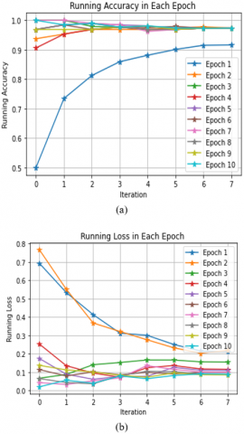
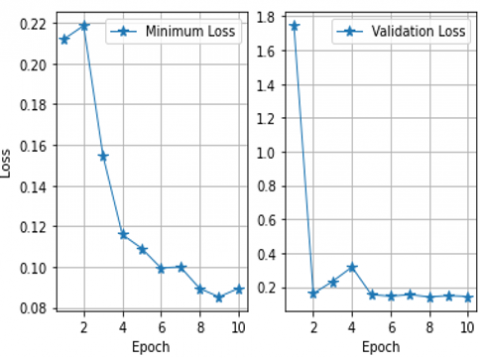
Subgraphs (a) and (b) of Figure 21 illustrate the model's performance by evaluating the running accuracy and loss. Additionally, Figure 22 illustrates the minimum loss and validation loss. The model was ultimately saved with a minimum loss of 0.0816 and an accuracy of 0.9736.
Figure 21. Loss and accuracy progression throughout each iteration in every epoch
Figure 22. Minimum loss and validation loss sequentially in each epoch
The performance of the proposed work in terms of processing time elapsed/step with validation loss and validation accuracy is depicted in Table 9 and Table 10. It can be observed that as epoch increases elapsed time/step decreases, and the model ultimately achieves its optimum accuracy at iteration 2.
In addition to the performance showcased in the preceding figures and tables, the author assessed the effectiveness of the proposed approach against ten alternative methods. The comparative analysis of accuracy with these ten approaches is presented in Table 11 and Figure 23 revealing that the performance of the proposed work surpasses that of the other ten methods.
Table 9. Performance in terms of processing time per step with loss and accuracy in each epoch during Iteration 1
|
Epoch |
Iteration 1 |
||
|
Time / Step |
Loss |
Accuracy |
|
|
Epoch 1 |
5s 245 ms |
0.3186 |
0.8590 |
|
Epoch 2 |
1s 153 ms |
0.1622 |
0.9736 |
|
Epoch 3 |
1s 156 ms |
0.1179 |
0.9736 |
|
Epoch 4 |
1s 155 ms |
0.1055 |
0.9736 |
|
Epoch 5 |
1s 157 ms |
0.1113 |
0.9736 |
|
Epoch 6 |
1s 159 ms |
0.0961 |
0.9736 |
|
Epoch 7 |
1s 158 ms |
0.0922 |
0.9736 |
|
Epoch 8 |
1s 158 ms |
0.0850 |
0.9736 |
|
Epoch 9 |
1s 155 ms |
0.0834 |
0.9736 |
|
Epoch 10 |
1s 155 ms |
0.1305 |
0.9646 |
Table 10. Performance in terms of processing time per step with loss and accuracy in each epoch during Iteration 2
|
Epoch |
Iteration 2 |
||
|
Time / Step |
Loss |
Accuracy |
|
|
Epoch 1 |
4s 223 ms |
0.3274 |
0.9207 |
|
Epoch 2 |
1s 147 ms |
0.1468 |
0.9736 |
|
Epoch 3 |
1s 145 ms |
0.1198 |
0.9736 |
|
Epoch 4 |
1s 158 ms |
0.1047 |
0.9736 |
|
Epoch 5 |
1s 161 ms |
0.1103 |
0.9736 |
|
Epoch 6 |
1s 160 ms |
0.0970 |
0.9736 |
|
Epoch 7 |
1s 155 ms |
0.1028 |
0.9736 |
|
Epoch 8 |
1s 158 ms |
0.0939 |
0.9736 |
|
Epoch 9 |
1s 166 ms |
0.0947 |
0.9736 |
|
Epoch 10 |
1s 159 ms |
0.0844 |
0.9736 |
Table 11. Comparison in terms of accuracy with the other ten approaches
|
Approach |
Accuracy |
|
SqueezeNet |
96.33% |
|
Random Forest (RF) |
94.53% |
|
Support Vector Machine (SVM) |
97.89% |
|
Speeded-Up Robust Features (SURF) Detector, Support Vector Machines |
91.70% |
|
Symmetrical SURF Descriptor |
91.10% |
|
Partial-Feature based Part-Based Model |
92.47% |
|
Bag of Speeded-Up Robust Features (BoSURF) |
94.84% |
|
Haar-like Features, AdaBoost, Gabor Wavelet Transform, Local Binary Pattern Operator, PCA |
91.60% |
|
Linear SVM Binary Classifier, HOG Features |
94.00% |
|
Harris Corner Strengths |
96.00% |
|
Proposed Work |
97.36% |
Figure 23. Performance of proposed work as compared to other approaches
5.2 Discussion
The use of a contour-based detection approach in the proposed methodology is justifiable for several reasons, despite the availability of state-of-the-art object detection algorithms. The choice of the proposed approach aligns with the specific objectives, dataset characteristics, and the challenges addressed in the research, particularly in the context of handling varying lighting conditions. The algorithms may exhibit sensitivity to certain conditions, adaptability, robustness to complex scenes, ability to handle occlusions, and computational efficiency. Moreover, they serve as a foundational step, paving the way for subsequent more specialized vehicle analyses and monitoring.
During the study, the author observed that the proposed approach is well suited for four-wheelers such as cars. Its accuracy on commercial vehicles, heavy vehicles such as trucks, and three-wheelers such as autos may vary because of their shape and size. Another challenge arises with identical vehicles, as in some cases, the commercial vehicle belongs to the same company, which is why they may be identical. Moreover, since a brand-new vehicle with the same company, same brand, and same color is identical, this is also a challenge.
Table 12 provides a detailed justification for this choice to show the performance of the proposed work under different scenarios.
Table 12. Justification of contour-based detection approach to perform under different scenarios
|
Parameters |
Justification |
|
Robustness to Complex Scenarios |
Contour-based detection algorithms are inherently versatile in handling complex scenarios. Unlike some algorithms that may rely on predefined patterns or features, contour-based methods are adaptive and can identify object edges even in challenging situations. |
|
Computational Efficiency |
The algorithms are often computationally efficient, making them suitable for near-real-time applications. They require fewer computational resources compared to some other deep learning-based methods, which can be advantageous in resource-constrained environments. This adaptability aligns with our methodology to detect the optimal position of the vehicle. |
|
Adaptability to Lighting Variations |
While it is true that contour-based algorithms can be sensitive to lighting conditions, they can still perform effectively with appropriate preprocessing (image enhancement and thresholding) and adaptive techniques to mitigate the impact of lighting variations. Furthermore, the methods can work well in scenarios where shadows or changing illumination patterns are present, which are common in real-world roadside traffic areas. |
|
Custom Dataset Considerations |
The custom dataset used in our study incorporates scenarios encountered in real-world traffic. Since contour-based detection is inherently well-suited for such scenarios, its selection was deliberate. |
|
Handling Occlusions |
The approach offers advantages when dealing with partial occlusions. In scenarios where vehicles are partially obscured by other objects or surroundings (e.g., trees or buildings), and can often still outline the visible portions of the vehicle, which is essential in traffic monitoring applications. |
|
Region of Interest (ROI) Extraction |
The approach facilitates the extraction of ROIs containing vehicles. These ROIs can subsequently be subjected to more focused and computationally intensive analysis, allowing for efficient resource allocation. |
In roadside traffic area surveillance, the positioning of vehicles within the camera frame is of utmost significance. Vehicle detection in roadside traffic monitoring videos plays a vital role in ITMS. To set up video surveillance at roadside traffic, locations of cameras, and other equipment, considering factors such as coverage area, camera angles, and lighting conditions matter. The widespread equipment of surveillance cameras has resulted in a vast database of traffic footage for analysis. Conventional surveillance is often hindered by distortions resulting from camera angles and lightning. However, when the cameras are positioned at a prominent viewing angle, the road appears more distant, which affects the size of the detected objects. Effectively addressing these challenges and finding solutions is essential, especially in complex camera scenes, to enable further practical applications. To tackle this issue, contour-based detection methods are utilized. These techniques concentrate on delineating the silhouette of vehicles, encompassing their distinctive features.
In summary, by addressing these challenges and finding the optimal vehicle position, this work not only advances the field of roadside traffic surveillance but also aligns with the broader goal of optimizing the smart city framework for enhanced functionality and contributes to the overall efficiency of smart city traffic management systems. These advancements not only address the specific challenges of road-side traffic surveillance but also contribute to the broader goal of creating more intelligent, efficient, and secure urban environments.
This manuscript introduces a lightweight CNN based on contour detection, specifically designed to contribute to transport development and integration. The proposed architecture focuses on vehicle detection and the extraction of crucial features, leveraging a custom dataset for maximum effectiveness. The analysis includes the evaluation and visualization of pixel distribution, pixel intensity, and video density through various plots and charts. The Structural Similarity Index (SSIM) is employed to compare frames in different positions, calculating parameters such as MSSIM, ssim_map, MLS, MCS, and MSS, along with PSNR for frame pairs (from frame 0 to 298), presented in tables and figures. The SSIM metric is used to assess how similar two images are to one another; it ranges in value from -1 to +1. The number +1 denotes that the two images are identical or extremely similar, whereas a value of -1 denotes that the two images are highly dissimilar. These numbers are frequently modified to fall inside the range [0, 1], where the extremes have the same significance. However, human visual perception excels at identifying structural details in a scene and discerning differences between the information extracted from reference and sample images. In the realm of practical real-life scenarios, the two different vehicles can look the same or the same vehicle can look different in different positions, illumination, and light intensity. Therefore, metrics that replicate this behavior tend to be more effective. Beyond assessing the proposed work's performance, a systematic literature survey incorporates comparisons with various models and approaches through tables, aligning with the goals of transport development and integration. The results demonstrate the efficacy of the proposed work under challenging conditions, including partial occlusions, poor visibility, varying light intensities, and diverse recording angles.
Despite outperforming previous works and approaches, there is still room for further improvement. Expanding the dataset and including a wider variety of vehicles could be beneficial for future research in this area. Future research in this area could benefit from incorporating a wider variety of vehicles to enhance the applicability of the proposed methodology in the context of transport development and integration.
This research was supported by Technosys Security System Pvt. Ltd. Bhopal, (Madhya Pradesh) India, under a research collaboration.
[1] Khanna, A., Goyal, R., Verma, M., Joshi, D. (2019). Intelligent traffic management system for smart cities. In: Singh, P., Paprzycki, M., Bhargava, B., Chhabra, J., Kaushal, N., Kumar, Y. (eds) Futuristic Trends in Network and Communication Technologies. FTNCT 2018. Communications in Computer and Information Science, 958: 152-164. Springer, Singapore. https://doi.org/10.1007/978-981-13-3804-5_12
[2] Yazici, A., Koyuncu, M., Sert, S.A., Yilmaz, T. (2019). A Fusion-based framework for wireless multimedia sensor networks in surveillance applications. IEEE Access, 7: 88418-88434. https://doi.org/10.1109/ACCESS.2019.2926206
[3] Hilmani, A., Maizate, A., Hassouni, L. (2020). Automated real-time intelligent traffic control system for smart cities using wireless sensor networks. Wireless Communications and Mobile Computing, 2020: 1-28. https://doi.org/10.1155/2020/8841893
[4] Fernández-Sanjurjo, M., Bosquet, B., Mucientes, M., Brea, V.M. (2019). Real-time visual detection and tracking system for traffic monitoring. Engineering Applications of Artificial Intelligence, 85: 410-420. https://doi.org/10.1016/j.engappai.2019.07.005
[5] Sharma, N.K., Rahamatkar, S., Rathore, A.S. (2022). Role and applications of emerging technologies in smart city architecture. In: Roy, B.K., Chaturvedi, A., Tsaban, B., Hasan, S.U. (eds) Cryptology and Network Security with Machine Learning. ICCNSML 2022. Algorithms for Intelligent Systems, pp. 2-14. Springer, Singapore. https://doi.org/10.1007/978-981-99-2229-1_1
[6] Bouhsissin, S., Sael, N., Benabbou, F. (2023). Evaluating data sources and datasets in intelligent transport systems through a weighted scoring model. International Journal of Transport Development and Integration, 7(4): 353-365. https://doi.org/10.18280/ijtdi.070409
[7] Adeliyi, T.T., Oluwadele, D., Igwe, K., Aroba, O.J. (2023). Analysis of road traffic accidents severity using a pruned tree-based model. International Journal of Transport Development and Integration, 7(2): 131-138. https://doi.org/10.18280/ijtdi.070208
[8] Di Gangi, M., Belcore, O.M., Polimeni, A. (2023). An overview on decision support systems for risk management in emergency conditions: present, past and future trends. International Journal of Transport Development and Integration, 7(1): 45-53. https://doi.org/10.18280/ijtdi.070106
[9] Manikandan, R., Ramakrishnan, R. (2013). Video object extraction by using background subtraction techniques for sports applications. Digital Image Processing, 5(9): 435-440.
[10] Liu, Y., Lu, Y., Shi, Q.X., Ding, J.H. (2013). Optical flow based urban road vehicle tracking. In 2013 Ninth International Conference on Computational Intelligence and Security, Emeishan, China, pp. 391-395. https://doi.org/10.1109/CIS.2013.89
[11] Zeng, J., Zhang, K., Wang, L., Li, J. (2023). FedLVR: A federated learning-based fine-grained vehicle recognition scheme in intelligent traffic system. Multimedia Tools and Applications, 82: 37431-37452. https://doi.org/10.1007/s11042-023-15004-w
[12] Zhang, Q., Zhuo, L., Zhang, S.Y., Li, J.F., Zhang, H., Li, X.G. (2018). Fine-grained vehicle recognition using lightweight convolutional neural network with combined learning strategy. In 2018 IEEE Fourth International Conference on Multimedia Big Data (BigMM), Xi'an, China, pp. 1-5. https://doi.org/10.1109/BigMM.2018.8499085
[13] Badura, P., Skotnicka, M. (2014). Automatic car make recognition in low-quality images. Information Technologies in Biomedicine, 3: 235-246.
[14] Llorca, D.F., Arroyo, R., Sotelo, M.A. (2013). Vehicle logo recognition in traffic images using HOG features and SVM. In 16th International IEEE Conference on Intelligent Transportation Systems (ITSC 2013), The Hague, Netherlands, pp. 2229-2234. https://doi.org/10.1109/ITSC.2013.6728559
[15] Baran, R., Glowacz, A., Matiolanski, A. (2015). The efficient real- and non-real-time make and model recognition of cars. Multimedia Tools and Applications, 74: 4269-4288. https://doi.org/10.1007/s11042-013-1545-2
[16] Bhatti, U.A., Yu, Z., Yuan, L., Nawaz, S.A., Aamir, M., Bhatti, M.A. (2022). A robust remote sensing image watermarking algorithm based on region-specific SURF. In Ullah, A., Anwar, S., Rocha, Á., Gill, S. (eds) Proceedings of International Conference on Information Technology and Applications. Lecture Notes in Networks and Systems, 350: 75-85. Springer, Singapore. https://doi.org/10.1007/978-981-16-7618-5_7
[17] Jagannathan, P., Rajkumar, S., Frnda, J., Divakarachari, P. B., Subramani, P. (2021). Moving vehicle detection and classification using gaussian mixture model and ensemble deep learning technique. Wireless Communications and Mobile Computing, 2021: 1-15. https://doi.org/10.1155/2021/5590894
[18] Bochkovskiy, A., Wang, C.Y., Liao, H.Y.M. (2020). YOLOv4: Optimal speed and accuracy of object detection. arXiv preprint arXiv:2004.10934. https://doi.org/10.48550/arXiv.2004.10934
[19] Redmon, J., Farhadi, A. (2018). YOLOv3: An incremental improvement. arXiv preprint arXiv: 1804.02767.https://doi.org/10.48550/arXiv.1804.02767
[20] Redmon, J., Farhadi, A. (2017). YOLO9000: Better, faster, stronger. In 2017 IEEE Conference on Computer Vision and Pattern Recognition (CVPR), Honolulu, HI, USA, pp. 6517-6525. https://doi.org/10.1109/CVPR.2017.690
[21] Yin, Y.H., Li, H.F., Fu, W. (2020). Faster-YOLO: An accurate and faster object detection method. Digital Signal Processing, 102: 102756. https://doi.org/10.1016/j.dsp.2020.102756
[22] Ahmad, T., Ma, Y., Yahya, M., Ahmad, B., Nazir, S., Haq, A. U., Ali, R. (2020). Object detection through modified YOLO neural network. Scientific Programming, 2020: 1-10. https://doi.org/10.1155/2020/8403262
[23] Tao, J., Wang, H.B., Zhang, X.Y., Li, X.Y., Yang, H.W. (2017). An object detection system based on YOLO in traffic scene. In 2017 6th International Conference on Computer Science and Network Technology (ICCSNT), Dalian, China, pp. 315-319. https://doi.org/10.1109/ICCSNT.2017.8343709
[24] Shaifee, M.J., Chywl, B., Li, F., Wong, A. (2017). Fast YOLO: A fast you only look once system for real-time embedded object detection in video. Journal of Computational Vision and Imaging Systems, 3(1). https://doi.org/10.15353/vsnl.v3i1.171
[25] Liu, S.H., Zha, J.L., Sun, J., Li, Z., Wang, G. (2023). EdgeYOLO: An edge-real-time object detector. arXiv preprint arXiv:2302.07483. https://doi.org/10.48550/arXiv.2302.0748
[26] Li, S.S., Li, Y.J., Li, Y., Li, M.J., Xu, X.R. (2021). YOLO-FIRI: Improved YOLOv5 for infrared image object detection. IEEE Access, 9: 141861-141875. https://doi.org/10.1109/ACCESS.2021.3120870
[27] Mao, Q.C., Sun, H.M., Liu, Y.B., Jia, R.S. (2019). Mini-YOLOv3: Real-time object detector for embedded applications. IEEE Access, 7: 133529-133538. https://doi.org/10.1109/ACCESS.2019.2941547
[28] Ren, S., He, K., Girshick, R., Sun, J. (2017). Faster R-CNN: Towards real-time object detection with region proposal networks. IEEE Transactions on Pattern Analysis and Machine Intelligence, 39(6): 1137-1149. https://doi.org/10.1109/TPAMI.2016.2577031
[29] Chen, Y.H., Li, W., Sakaridis, C., Dai, D.X., Van Gool, L. (2018). Domain adaptive faster R-CNN for object detection in the wild. In 2018 IEEE/CVF Conference on Computer Vision and Pattern Recognition, Salt Lake City, UT, USA, pp. 3339-3348. https://doi.org/10.1109/CVPR.2018.00352
[30] Benjdira, B., Khursheed, T., Koubaa, A., Ammar, A., Ouni, K. (2019). Car Detection using Unmanned Aerial Vehicles: Comparison between faster R-CNN and YOLOv3. In 2019 1st International Conference on Unmanned Vehicle Systems-Oman (UVS), Muscat, Oman, pp. 1-6. https://doi.org/10.1109/UVS.2019.8658300
[31] Maity, M., Banerjee, S., Sinha Chaudhuri, S. (2021). Faster R-CNN and YOLO based vehicle detection: A survey. In 2021 5th International Conference on Computing Methodologies and Communication (ICCMC), Erode, India, pp. 1442-1447. https://doi.org/10.1109/ICCMC51019.2021.9418274
[32] Wen, L.W., Ding, J.S., Loffeld, O. (2021). Video SAR moving target detection using dual faster R-CNN. IEEE Journal of Selected Topics in Applied Earth Observations and Remote Sensing, 14: 2984-2994. https://doi.org/10.1109/JSTARS.2021.3062176
[33] Salvador, A., Giro-I-Nieto, X., Marques, F., Satoh, S. (2016). Faster R-CNN features for instance search. In 2016 IEEE Conference on Computer Vision and Pattern Recognition Workshops (CVPRW), Las Vegas, NV, USA, 394-401. https://doi.org/10.1109/CVPRW.2016.56
[34] Liu, W., Anguelov, D., Erhan, D., Szegedy, C., Reed, S., Fu, C.Y., Berg, A.C. (2016). SSD: Single shot multibox detector. In Computer Vision–ECCV 2016: 14th European Conference, Amsterdam, The Netherlands, Proceedings, Part I, pp. 21-37. https://doi.org/10.1007/978-3-319-46448-0_2
[35] Leng, J.X., Liu, Y. (2021). Single-shot augmentation detector for object detection. Neural Computing and Applications, 33(8): 3583-3596. https://doi.org/10.1007/s00521-020-05202-0
[36] Wang, Y.Z., Niu, P.H., Guo, X.Y., Yang, G.W., Chen, J. (2021). Single shot multibox detector with deconvolutional region magnification procedure. IEEE Access, 9: 47767-47776. https://doi.org/10.1109/ACCESS.2021.3068486
[37] Li, W.Q., Liu, G.Z. (2019). A single-shot object detector with feature aggregation and enhancement. In 2019 IEEE International Conference on Image Processing (ICIP), pp. 3910-3914. https://doi.org/10.1109/ICIP.2019.8803543
[38] He, K.M., Gkioxari, G., Dollár, P., Girshick, R. (2020). Mask R-CNN. IEEE Transactions on Pattern Analysis and Machine Intelligence, 42(2): 386-397. https://doi.org/10.1109/TPAMI.2018.2844175
[39] Hu, R.H., Dollar, P., He, K.M., Darrell, T., Girshick, R. (2018). Learning to segment every thing. In 2018 IEEE/CVF Conference on Computer Vision and Pattern Recognition, Salt Lake City, UT, USA, pp. 4233-4241. https://doi.org/10.1109/CVPR.2018.00445
[40] Kirillov, A., Wu, Y.X,, He, K.M.,Girshick, R. (2020). Pointrend: Image segmentation as rendering. In 2020 IEEE/CVF Conference on Computer Vision and Pattern Recognition (CVPR), Seattle, WA, USA, pp. 9796-9805. https://doi.org/10.1109/CVPR42600.2020.00982
[41] Tan, M.X., Pang, R.M., Le, Q. V. (2020). EfficientDet: Scalable and efficient object detection. In 2020 IEEE/CVF Conference on Computer Vision and Pattern Recognition (CVPR), Seattle, WA, USA, pp. 10778-10787. https://doi.org/10.1109/CVPR42600.2020.01079
[42] Jia, J.Q., Fu, M., Liu, X.F., Zheng, B. (2022). Underwater object detection based on improved EfficientDet. Remote Sens, 14(18): 4487. https://doi.org/10.3390/rs14184487
[43] Duan, K.W., Bai, S., Xie, L.X., Qi, H.G., Huang, Q.M., Tian, Q. (2019). CenterNet: Keypoint triplets for object detection. Proceedings of the IEEE International Conference on Computer Vision, 2019-Octob(Iccv), pp. 6568-6577. https://doi.org/10.1109/ICCV.2019.00667
[44] Anagnostopoulos, C.N.E., Anagnostopoulos, I.E., Psoroulas, I.D., Loumos, V., Kayafas, E. (2008). License plate recognition from still images and video sequences: A survey. IEEE Transactions on Intelligent Transportation Systems, 9(3): 377-391. https://doi.org/10.1109/TITS.2008.922938
[45] Gnanaprakash, V., Kanthimathi, N., Saranya, N. (2021). Automatic number plate recognition using deep learning. IOP Conference Series: Materials Science and Engineering, 1084(1): 012027. https://doi.org/10.1088/1757-899x/1084/1/012027
[46] Ammar, A., Koubaa, A., Boulila, W., Benjdira, B., Alhabashi, Y. (2023). A multi-stage deep-learning-based vehicle and license plate recognition system with real-time edge inference. Sensors, 23(4): 2120. https://doi.org/10.3390/s23042120
[47] Puarungroj, W., Boonsirisumpun, N. (2018). Thai license plate recognition based on deep learning. Procedia Computer Science, 135: 214-221. https://doi.org/10.1016/j.procs.2018.08.168
[48] Ghahremannezhad, H., Shi, H., Liu, C.J. (2023). Object detection in traffic videos: A survey. IEEE Transactions on Intelligent Transportation Systems, 24(7): 6780-6799. https://doi.org/10.1109/TITS.2023.3258683
[49] Song, H.S., Liang, H.X., Li, H.Y., Dai, Z., Yun, X. (2019). Vision-based vehicle detection and counting system using deep learning in highway scenes. European Transport Research Review, 11: 51. https://doi.org/10.1186/s12544-019-0390-4
[50] Mithun, N.C., Munir, S., Guo, K., Shelton, C. (2018). ODDS: Real-time object detection using depth sensors on embedded GPUs. In 2018 17th ACM/IEEE International Conference on Information Processing in Sensor Networks (IPSN), Porto, pp. 230-241. https://doi.org/10.1109/IPSN.2018.00051
[51] Jolly, M.P.D., Lakshmanan, S., Jain, A.K. (1996). Vehicle segmentation and classification using deformable templates. IEEE Transactions on Pattern Analysis and Machine Intelligence, 18(3): 293-308. https://doi.org/10.1109/34.485557
[52] Szwoch, G., Dalka, P. (2014). Detection of Vehicles stopping in restricted zones in? Video from surveillance cameras. Communications in Computer and Information Science, 429: 242-253. https://doi.org/10.1007/978-3-319-07569-3_20
[53] Ali, M.D.H., Kurokawa, S., Shafie, A.A. (2013). Autonomous road surveillance system: A proposed model for vehicle detection and traffic signal control. Procedia Computer Science, 19: 963-970. https://doi.org/10.1016/j.procs.2013.06.134
[54] Wang, Z.G., Zhan, J., Duan, C.G., Guan, X., Lu, P.P., Yang, K. (2022). A Review of vehicle detection techniques for intelligent vehicles. IEEE Transactions on Neural Networks and Learning Systems, 34(8): 1-21. https://doi.org/10.1109/TNNLS.2021.3128968
[55] Lee, H.J., Ullah, I., Wan, W., Gao, Y.B., Fang, Z.J. (2019). Real-time vehicle make and model recognition with the residual squeezenet architecture. Sensors, 19(5): 982. https://doi.org/10.3390/s19050982
[56] Siddiqui, A. J., Mammeri, A., Boukerche, A. (2016). Real-time vehicle make and model recognition based on a bag of SURF features. IEEE Transactions on Intelligent Transportation Systems, 17(11): 3205-3219. https://doi.org/10.1109/TITS.2016.2545640
[57] Chen, L.C., Hsieh, J.W., Yan, Y.L., Chen, D.Y. (2013). Vehicle make and model recognition using sparse representation and symmetrical SURFs. In 16th International IEEE Conference on Intelligent Transportation Systems (ITSC 2013), The Hague, Netherlands, pp. 1143-1148. https://doi.org/10.1109/ITSC.2013.6728386
[58] Ros, G., Alvarez, J.M. (2015). Unsupervised image transformation for outdoor semantic labelling. In 2015 IEEE Intelligent Vehicles Symposium (IV), Seoul, Korea (South), pp. 537-542. https://doi.org/10.1109/IVS.2015.7225740
[59] Ros, G., Ramos, S., Granados, M., Bakhtiary, A., Vazquez, D., Lopez, A.M. (2015). Vision-based offline-online perception paradigm for autonomous driving. In 015 IEEE Winter Conference on Applications of Computer Vision, Waikoloa, HI, USA, pp. 231-238. https://doi.org/10.1109/WACV.2015.38
[60] Zhang, R., Candra, S.A., Vetter, K., Zakhor, A. (2015). Sensor fusion for semantic segmentation of urban scenes. In 2015 IEEE International Conference on Robotics and Automation (ICRA), Seattle, WA, USA, pp. 1850-1857. https://doi.org/10.1109/ICRA.2015.7139439
[61] Sturgess, P., Alahari, K., Ladický, L., Torr, P.H.S. (2009). Combining appearance and structure from motion features for road scene understanding. In BMVC - British Machine Vision Conference, London, United Kingdom. https://doi.org/10.5244/C.26.127
[62] Brostow, G.J., Fauqueur, J., Cipolla, R. (2009). Semantic object classes in video: A high-definition ground truth database. Pattern Recognition Letters, 30(2): 88-97. https://doi.org/10.1016/j.patrec.2008.04.005
[63] Cordts, M., Omran, M., Ramos, S., Rehfeld, T., Enzweiler, M., Benenson, R., Franke, U., Roth, S., Schiele, B. (2016). The cityscapes dataset for semantic urban scene understanding. In 2016 IEEE Conference on Computer Vision and Pattern Recognition (CVPR), Las Vegas, NV, USA, pp. 3213-3223. https://doi.org/10.1109/CVPR.2016.350
[64] Luo, Z.M., Branchaud-Charron, F., Lemaire, C., Konrad, J., Li, S.Z., Mishra, A., Achkar, A., Eichel, J., Jodoin, P.M. (2018). MIO-TCD: A new benchmark dataset for vehicle classification and localization. IEEE Transactions on Image Processing, 27(10): 5129-5141. https://doi.org/10.1109/TIP.2018.2848705
[65] Lin, T.Y., Maire, M., Belongie, S., Hays, J., Perona, P., Ramanan, D., … Zitnick, C.L. (2014). Microsoft coco: Common objects in context. In Computer Vision-ECCV 2014: 13th European Conference, Zurich, Switzerland, Proceedings, Part V, pp. 740-755. https://doi.org/10.1007/978-3-319-10602-1_48
[66] Leal-Taixé, L., Milan, A., Reid, I., Roth, S., Schindler, K. (2015). Motchallenge 2015: Towards a benchmark for multi-target tracking. arXiv preprint arXiv:1504.01942. https://doi.org/10.48550/arXiv.1504.01942
[67] Wang, Z., Bovik, A.C., Sheikh, H.R., Simoncelli, E.P. (2004). Image quality assessment: From error visibility to structural similarity. IEEE Transactions on Image Processing, 13(4): 600-612. https://doi.org/10.1109/TIP.2003.819861