Nadheer S. Ayoob*![]() | Ruqayah K. Mohammed
| Ruqayah K. Mohammed![]()
© 2025 The authors. This article is published by IIETA and is licensed under the CC BY 4.0 license (http://creativecommons.org/licenses/by/4.0/).
OPEN ACCESS
Evaluating the spatial and temporal evolutionary patterns of future rainfall and temperature at a basin scale under different emission scenarios is essential for formulating sustainable responses to climate change. Nevertheless, research in Iraq has not extensively addressed this issue. The aim of this study is to investigate the spatial and temporal properties of minimum and maximum temperatures as well as rainfall in the Little Zab River Watershed (LZRW) using the LARS-WG 8 model. Five General Circulation Models (GCMs) and two emission scenarios were used to project the weather variables for three projection periods (2041-2060, 2061-2080, and 2081-2100). Satellite data from 1985 to 2015 were used from ten meteorological stations adjacent to the watershed to perform model calibration and validation. Analysis of the results revealed that both minimum and maximum temperatures exhibited increasing trends during the projection periods, with a higher rate of increase for the minimum temperature. The SSP5-8.5 showed that the mean minimum and maximum temperatures increased by 58.09 and 26.65%, respectively, for the third period compared to the baseline values. Furthermore, the projected rainfall exhibited an unsteady increasing trend. The most significant rainfall increment (9.35%) was projected by the SSP2-4.5 for the period 2041-2060.
statistical downscaling, LARS-WG, SSP, LZRW, climate change
Climate change is identified as one of the most significant environmental challenges confronting the globe today, as mentioned in the Sixth Assessment Report (AR6) released by the Intergovernmental Panel on Climate Change (IPCC) [1]. The report stated that the surface temperature of the globe rose by 1.1℃ by 2020 relative to the levels from 1850 to 1900. This increasing pattern is anticipated to continue until the beginning of the 22nd century, reaching 1.5℃ [2, 3]. The impacts of climate change have been observed in numerous regions worldwide, including elevated temperatures, sea-level rise, ice melting, and degradation of air quality [4]. These effects are acknowledged as the most significant threat to human existence and livelihood on Earth [1, 2, 5]. The leading cause of climate change is the emission of greenhouse gases (GHG) due to the utilization of fossil fuels and alterations in land use/ land cover. The consequences of global warming are expected to worsen in the future, exerting a significant impact on hydrological processes [6].
The Middle East has been significantly impacted by global climate change because of its arid and semi-arid environment [7]. Iraq is one of the countries in the Middle East that has been most severely affected by climate change. Accordingly, Iraq will encounter significant environmental issues, including sudden floods, water shortages, sandstorms, and heatwaves [8]. Abdulsahib et al. [2], Hassan and Hashim [9], Mohammed and Fallah [10] revealed that extreme events are anticipated to increase in Middle Eastern countries due to the impacts of climate change.
Scientists frequently employ General Circulation Models (GCMs) to simulate and project climatic conditions under different emission scenarios [11]. The GCMs are numerical models with outputs of inferior spatial resolution. Thus, the GCMs' results cannot be employed directly to examine the effects of climate change. Consequently, downscaling methods must be applied to enhance the spatial resolution of the data [12, 13]. Downscaling techniques are classified into two categories: dynamic and statistical. An overview of downscaling methods was provided by Trzaska and Schnarr [14]. The GCM outcomes generated by the CMIP, an abbreviation for the Coupled Model Intercomparison Project, are the most widely applied [15-17]. The Working Group on Coupled Modelling (WGCM) has introduced the latest CMIP6 scenarios, which involve the most recent set of emission scenarios referred to as shared socio-economic pathways (SSPs), based on various socio-economic assumptions [2]. The Long Ashton Research Stations Weather Generator (LARS-WG) software is one of the most common Statistical Downscaling (SD) methods that reliably identifies complex patterns in spatial-temporal data prediction. The LARS-WG model requires fewer computational resources and provides a user-friendly interface compared to dynamical downscaling methods [1, 2].
The LARS-WG model has been effectively applied in various parts of the globe [11, 18-21]. Several investigations in this regard were carried out in Iraq. Mohammed et al. [22] applied LARS-WG to examine the impacts of climate change on ten weather stations around the Lower Zab River Basin in northeastern Iraq. Mohammed and Hassan [1] utilized LARS-WG 6 to predict changes in temperature and precipitation in southern Iraq under RCP4.5 and RCP8.5 over the three periods from 2021 to 2100. Abdulsahib et al. [2] used LARS-WG 8 to predict climate variables from 2021 to 2040 in northern Iraq by two scenarios (SSP2-4.5 and SSP5-8.5). The results of these studies revealed a continuous rise in minimum and maximum temperatures, while the rainfall trend exhibited noticeable fluctuation depending on the region, scenario, and period.
The Little Zab River (LZR), also known as the Lesser or Lower Zab, represents the Tigris River's second major tributary within Iraqi lands [23]. The length of the river is about 375 km. The LZR has a catchment area of 20000 km2 located in northeastern Iraq and northwestern Iran [24-26]. In addition to supplying the Tigris River, the Little Zab River Watershed (LZRW) is a significant area for agricultural and natural resources [25]. Throughout the 20th century, the LZRW has been significantly affected by conflicts, population growth, and climate change [27].
Although many researchers have conducted studies on climate change and forecasting climate factors in Iraq, including [28-30], there is a lack of thorough studies showing the impact of climate change and its repercussions on the watershed scale. Thus, the current study aims to project precipitation, minimum, and maximum temperature in the LZRW for three future periods: 2041-2060, 2061-2080, and 2081-2100. The LARS-WG 8 model was applied to project the climatic factors for 10 weather stations adjacent to the LZRW using five GCMs and two emission scenarios (SSP5-8.5 and SSP2-4.5). The Kriging tool in ArcMap 10.2 was used to convert the point data source at the weather station into a spatial map covering the LZRW. The research methodology employed will provide a precise vision of the extent to which each part of the study area is affected by climate change impacts. The results of this study will provide policymakers with a strong tool for fulfilling the requirement of sustainable natural and water resources within the basin.
2.1 Study area and data set
The Little Zab River Watershed (LZRW) (Figure 1) comprises numerous substantial drainage basins characterized by diverse climatic and hydrological circumstances. The lower and upper parts of the basin differ considerably, resulting in a much broader range of uncertainties about the impact of climate change on water resources availability [29]. The basin's topography ranges from flat terrain in the southeast to high mountains in the northeast [31]. The range of the basin's elevation is between 120 and 3600 m above mean sea level. The LZRW has an arid to semi-arid climate. The mean annual temperature ranges from 10 to 25℃ [25]. The annual rainfall over the watershed ranges from 1 m/year in the northeastern parts to less than 0.2 m/year in the southwest [32]. Approximately 90% of the annual rainfall occurs between November and April [33].
The daily climatic data from 10 meteorological stations located adjacent to the LZRW, spanning 31 years (1985-2015), were used to project the future rainfall, minimum, and maximum temperature for three future periods. The elevation of the stations shown in Figure 1 ranges from 306 m (Makhmoor) to 1536 m (Sachez).
Figure 1. Study area and the location of weather stations
The deficiency of continuous daily weather data from ground stations is a crucial issue in developing nations. The meteorological data from 1990 to 2018 are discontinuous because of the extraordinary conditions of terrorism and conflict in Iraq [2]. Tayyeh and Mohammed [34] stated that satellite data can be regarded as efficient and promising for hydrological and climatic research. Furthermore, satellite data have been effectively utilized to forecast future climatic data in various research studies, including [35, 36]. Thus, satellite-based weather data were used in this study. The daily temperature data were downloaded from https://power.larc.nasa.gov, while the precipitation data were downloaded from https://www.chc.ucsb.edu (CHIRPS).
Before applying the climatic data, statistical measures were used to assess the degree of correspondence between the satellite data and the available weather stations. The daily minimum temperatures obtained from NASA for the Kirkuk station, spanning from 1981 to 2001, were compared with the recorded data [37]. The statistical measures used (i.e., R2, PBIAS, and NSE) showed good to very good results.
Regarding the precipitation data, the analysis of NASA's data indicated unsatisfactory results. Consequently, the researchers pursued an alternative source of data, CHIRPS. Monthly-averaged precipitation data from 1980 to 2002 were examined at four weather stations: Erbil, Sulaymaniah, Salahaddin, and Kirkuk. The statistical indices exhibited very good to excellent results. Details for the weather stations used are shown in Table 1.
Table 1. Details of the weather station
|
No. |
Station |
Longitude )°( |
Latitude )°( |
Elevation )ma( |
|
1 |
Chemchamal |
44.83 |
35.52 |
701 |
|
2 |
Erbeel |
44.00 |
36.15 |
1088 |
|
3 |
Halabcha |
45.94 |
35.18 |
651 |
|
4 |
Kirkuk |
44.40 |
35.47 |
319 |
|
5 |
Mahabad |
45.70 |
36.75 |
1356 |
|
6 |
Makhmoor |
43.60 |
35.75 |
306 |
|
7 |
Sachez |
46.26 |
36.25 |
1536 |
|
8 |
Salahddin |
44.20 |
36.38 |
1088 |
|
9 |
Soran |
44.63 |
36.87 |
1132 |
|
10 |
Sulaymaniyah |
45.45 |
35.53 |
885 |
a above mean sea level
2.2 Using LARS-WG for downscaling
The LARS-WG, a widely used model for stochastic weather generation, was used to downscale the outputs of the GCMs. The model generates daily precipitation, temperature (maximum and minimum), and solar radiation at a specific location for present and future periods [38]. The first version of LARS-WG was released in 1990 by the Assessment of Agricultural Risk Project (Hungary). Semenov et al. [38], Babaeian and Najafi [39] investigated and confirmed the efficiency of the model at 18 weather stations in the USA, Asia, and Europe. In general, three steps are required to generate synthetic climatic data using the LARS-WG software, involving calibration and validation of the model, followed by data generation [2]. First, the model requires calibration. The ''Site Analysis" function evaluates the recorded meteorological data, including precipitation and both maximum and minimum temperatures, to determine their statistical characteristics. Secondly, throughout the model validation, the parameter files derived from the observed data in the calibration stage are used to generate synthetic meteorological data having the same statistical properties. To compare the probability distributions of simulated and actual meteorological data at the station under investigation, the Kolmogorov-Smirnov (K-S) goodness-of-fit test was used. Finally, the calibration parameter files are used to generate synthetic data similar to the GCM-simulated scenario [2, 40].
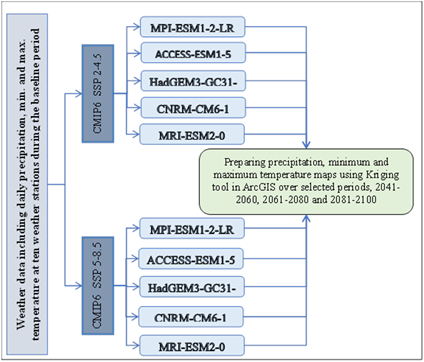
Figure 2. A flowchart explains the study's methodology
Figure 2 illustrates the methodology of the current study. The most recent LARS-WG model (i.e., 8.0) was employed with two SSPs to downscale the coarse-scale temperature and precipitation data obtained from five GCMs. The main steps in generating synthetic temperature and rainfall data were model calibration and validation, as well as obtaining climate weather data. Model calibration was performed using the baseline data from 1985 to 2015 (31 years) at the ten weather stations. The K-S test was used to assess the model's efficiency. The test was used to determine whether the seasonal distribution of the wet and dry series (WDS), the distribution of the daily maximum and minimum temperatures (TmaxD and TminD), and the distribution of daily precipitation (PD) derived from downscaled and observed data are the same [2]. The final stage is to produce future climatic data sets. In the current investigation, three future periods were studied (2041-2060, 2061-2080, and 2081-2100).
Tables 2 and 3 present the five GCMs and the two scenarios used in this study to project maximum and minimum temperatures, as well as rainfall. Applying a single GCM cannot precisely project future climatic data [41]. The average ensemble of GCMs results may provide precise estimations. Applying more than one GCM eliminates GCM biases and reduces uncertainties [42]. Thus, such a technique enables more reliable projections [43].
Table 2. The GCMs used in this study
|
No. |
GCM Models |
Institution |
Resolution (°) |
|
1 |
MRI-ESM2-0 |
Meteorological Research Institute, Tsukuba, Japan. |
1.1 × 11. |
|
2 |
CNRM-CM6-1 |
Centre National de Recherche Meteorologiques, Toulouse, France. |
1.4 × 1.4 |
|
3 |
ACCESS-ESM1-5 |
Australian Community Climate and Earth System Simulator, Acton, Australia. |
1.9 × 1.2 |
|
4 |
HasGEM3-GC31-LL |
Met Office, United Kingdom. |
1.8 × 1.2 |
|
5 |
MPI-ESM1-2-LR |
Max Planck Institute, Hamburg, Germany. |
1.9 × 1.9 |
Table 3. The two scenarios used in this study
|
No. |
SSP |
Description |
|
1 |
SSP2-4.5 |
Moderate greenhouse gas emissions: Carbon dioxide emissions will continue at present concentrations until 2050, then decrease, but not entirely vanish by 2100. |
|
2 |
SSP5-8.5 |
Exceedingly high greenhouse gas emissions: By 2075, Carbon dioxide emissions are projected to increase fourfold. |
3.1 Calibration and validation of the LARS-WG
The daily rainfall and temperature data from the ten weather stations associated with the LZRW, spanning from 1985 to 2015, were used for model calibration and validation. The model's efficiency in downscaling the GCMs' outputs in the study region was evaluated by statistical tests. The K-S test was used to verify the similarity of the daily weather data distribution derived from observed and simulated data. Furthermore, this research employed a p-value test to determine whether the hypothesis that both data sets (observed and projected) may have the same distribution. The simulated data is considered identical to the measured data if the p-value is high and the K-S value is low [2, 44]. The statistical indices calculated for the Halabcha station, as an example, are shown in Table 4.
Table 4. The K-S test and p-value for Halabcha station
|
A. K-S Test for Seasonal WDS Distributions |
|||||
|
Season |
Wet/Dry |
N |
K-S |
p-value |
Evaluation |
|
Dec. to Feb. |
Wet |
11.5 |
0.037 |
1.000 |
P |
|
dry |
11.5 |
0.050 |
1.000 |
P |
|
|
Mar. to May |
Wet |
11.5 |
0.038 |
1.000 |
P |
|
Dry |
11.5 |
0.074 |
1.000 |
P |
|
|
Jun. to Aug. |
Wet |
11.5 |
0.000 |
1.000 |
P |
|
Dry |
11.5 |
0.131 |
0.982 |
VG |
|
|
Sep. to Nov. |
Wet |
11.5 |
0.065 |
1.000 |
P |
|
Dry |
11.5 |
0.152 |
0.934 |
VG |
|
|
B. K-S Test for Daily Tmax Distribution |
|||||
|
Month |
N |
K-S |
p-value |
Evaluation |
|
|
Jan. |
11.5 |
0.106 |
0.999 |
VG |
|
|
Feb. |
11.5 |
0.053 |
1.000 |
P |
|
|
Mar. |
11.5 |
0.053 |
1.000 |
P |
|
|
Apr. |
11.5 |
0.053 |
1.000 |
P |
|
|
May |
11.5 |
0.053 |
1.000 |
P |
|
|
Jun. |
11.5 |
0.053 |
1.000 |
P |
|
|
Jul. |
11.5 |
0.053 |
1.000 |
P |
|
|
Aug. |
11.5 |
0.053 |
1.000 |
P |
|
|
Sep. |
11.5 |
0.053 |
1.000 |
P |
|
|
Oct. |
11.5 |
0.053 |
1.000 |
P |
|
|
Nov. |
11.5 |
0.033 |
1.000 |
P |
|
|
Dec. |
11.5 |
0.053 |
1.000 |
P |
|
|
C. K-S Test for Daily Tmin Distribution |
|||||
|
Month |
N |
K-S |
p-value |
Evaluation |
|
|
Jan. |
11.5 |
0.106 |
0.999 |
VG |
|
|
Feb. |
11.5 |
0.053 |
1.000 |
P |
|
|
Mar. |
11.5 |
0.053 |
1.000 |
P |
|
|
Apr. |
11.5 |
0.053 |
1.000 |
P |
|
|
May |
11.5 |
0.053 |
1.000 |
P |
|
|
Jun. |
11.5 |
0.106 |
0.999 |
VG |
|
|
Jul. |
11.5 |
0.053 |
1.000 |
P |
|
|
Aug. |
11.5 |
0.053 |
1.000 |
P |
|
|
Sep. |
11.5 |
0.053 |
1.000 |
P |
|
|
Oct. |
11.5 |
0.053 |
1.000 |
P |
|
|
Nov. |
11.5 |
0.053 |
1.000 |
P |
|
|
Dec. |
11.5 |
0.053 |
1.000 |
P |
|
|
D. K-S Test for Daily Rainfall Distribution |
|||||
|
Month |
N |
K-S |
p-value |
Evaluation |
|
|
Jan. |
11.5 |
0.130 |
0.984 |
VG |
|
|
Feb. |
11.5 |
0.130 |
0.984 |
VG |
|
|
Mar. |
11.5 |
0.065 |
1.000 |
P |
|
|
Apr. |
11.5 |
0.065 |
1.000 |
P |
|
|
May |
11.5 |
0.130 |
0.984 |
VG |
|
|
Jun. |
11.5 |
0.150 |
0.891 |
VG |
|
|
Jul. |
11.5 |
0.138 |
0.941 |
VG |
|
|
Aug. |
11.5 |
0.130 |
0.984 |
VG |
|
|
Sep. |
11.5 |
0.152 |
0.934 |
VG |
|
|
Oct. |
11.5 |
0.130 |
0.984 |
VG |
|
|
Nov. |
11.5 |
0.070 |
1.000 |
P |
|
|
Dec. |
11.5 |
0.130 |
0.984 |
VG |
|
According to Semenov and Barrow [45], the fit is poor if the p-value is less than 0.4. For 0.4 ≤ p-value < 0.7 and 0.7 ≤ p-value < 1.0, the fit is considered good and very good, respectively, while a perfect fit is achieved for p-value equal to 1.0. The evaluation results displayed in Table 4 indicate that the model's performance in predicting the distribution of daily Tmax, Tmin, and rainfall is perfect (P), with occasional instances of very good (VG) results. As a result, the downscaling technique was employed with more confidence in this study.
Additional statistical indicators were used to assess the performance of the LARS-WG model in Halabcha station. The indicators applied are the root mean square error (RMSE), coefficient of determination (R2), and mean bias error (MBE) [1, 2].
RMSE is a model evaluation statistic that works as an error index. The nearer the RMSE is to zero, the higher the model's efficiency:
$RMSE=\sqrt{\frac{\mathop{\sum }_{1}^{n}{{\left( {{G}_{i}}-{{O}_{i}} \right)}^{2}}}{n}}$ (1)
R2 signifies a relativity coefficient that spans from zero to unity, with the optimal value being 1:
${{R}^{2}}=\frac{\mathop{\sum }_{1}^{n}{{G}_{i}}{{O}_{i}}}{\sqrt{\mathop{\sum }_{1}^{n}G_{i}^{2}\mathop{\sum }_{1}^{n}O_{i}^{2}}}$ (2)
MBE signifies the error in the model estimation. It may possess either a negative or a positive value. Nevertheless, the optimal value is zero:
$MBE=~\frac{\mathop{\sum }_{1}^{n}\left( {{G}_{i}}-{{O}_{i}} \right)}{n}$ (3)
where $G_i$ is the generated value of the weather variable, $O_i$ is the observed value, and $n$ is the data number.
The results (Table 5) revealed that the LARS-WG model can effectively predict weather variables. The statistical criteria demonstrated a good agreement between the observed and generated data, as the indicators determined were within acceptable limits [46, 47].
Table 5. Statistical indicators result for model calibration and validation during the baseline period
|
Climatic Variable |
RMSE |
R2 |
MBE |
|
Tmin |
0.679 |
0.995 |
-0.056 |
|
Tmax |
0.818 |
0.999 |
-0.061 |
|
Rainfall |
0.490 |
0.970 |
0.033 |
3.2 Projection results
The calibration and validation results obtained from the LARS-WG model indicated that its effectiveness was sufficient for downscaling and predicting daily precipitation and temperature (minimum and maximum) at the ten weather stations. Consequently, the calibrated model was used to forecast the daily climatic variables for each station over the three intervals (i.e., 2041-2060, 2061-2080, and 2081-2100) using five GCMs and two scenarios.
A prevalent method in climate change effect research is to evaluate the phenomenon at a specific location separately [1, 13, 30, 48]. Abdulsahib et al. [2], Noor et al. [49] displayed the phenomenon spatially using the Inverse Distance Weighted (IDW). In this study, the Kriging tool in ArcGIS software was employed to create the spatial-temporal maps of the climatic variables. Kriging is a geostatistical prediction technique that generates weights from adjacent known values to estimate values at unmeasured sites [50]. Amelia et al. [51] and Shi et al. [52] stated that Kriging is superior to IDW, as it exhibits the highest interpolation accuracy and effectively captures the changing trends of precipitation across extensive areas. Additionally, Abdulsahib et al. [2] stated that the bull's-eye effect is one of the IDW's defects which can be overcome using the Kriging tool.
According to the author's cartographic skills and previous works [2, 53], the following points were considered while preparing the maps: (1) the weather variables were divided into five classes, choosing smaller and larger number of classes makes the maps uninformative or confusing, respectively, (2) the lowest and highest possible values of the weather variable of all scenarios and future periods were determined to fix the classes across all maps, enabling the reader to compare the results by simply seeing the maps, and (3) the classes' coverage percentage (%) relative to the entire area was calculated and written for each class.
3.2.1 Projection of minimum temperature
The spatial maps of the annual average minimum temperature (Tmin) for the LZRW are displayed in Figures 3 to 5. For all the figures, the minimum temperatures were equally divided into five classes, ranging from class 6-9℃ (the lowest) to class 18-21°C (the highest). Figure 3 shows the mean Tmin maps during the first future period (2041-2060) using the two scenarios (SSP 2-4.5 and SSP 5-8.5) compared to the observed map (1985-2015). The observed map involved the first three classes. The eastern parts of the watershed exhibited the lowest temperatures (class 6-9℃), followed by the central and western parts. The projected maps indicated an increase in the minimum temperature as a new class (15-18℃) appeared and covered the western areas. In the SSP 2-4.5 map, the extent of class 6-9℃ reduced from 38.32% in the observed map to 4.87%, while class 15-18℃ increased from 0% to 26.74%. It can be observed that the coldest class (6-9℃) disappeared in the SSP5-8.5 map, and the map was approximately similar to the observed map, but with one class shifting. In other words, the area of class 6-9℃ was covered by the higher class (9-12℃) and so on.
Figure 3. Results of minimum temperatures for the observed and projected maps (2041-2060)
Figure 4. Results of minimum temperatures for the observed and projected maps (2061-2080)
The comparison between the Tmin of the baseline period and the projection results for the second future period is shown in Figure 4. The figure indicated a continuous rise in Tmin from 2061 to 2080 across the LZRW. The most significant increase can be observed in the SSP5-8.5 map, where the hottest class (18-21℃) covered 20.72% of the basin. Furthermore, one can notice that the SSP2-4.5 map is approximately similar to that of the SSP5-8.5 in the first period.
Figure 5 depicts the effect of climate change on the minimum temperature at the LZRW during the third period (2081-2100). The same increasing trend can be observed within the basin. The predominant class in the central part, for instance, of the basin during the baseline period was class 9-12℃, while it shifted to class 12-15℃ and 15-18℃ in the maps of the SSP2-4.5 and SSP5-8.5, respectively.
Figure 5. Results of minimum temperatures for the observed and projected maps (2081-2100)
Figure 6 summarizes the predicted effects of climate change on the minimum temperature within the LZRW. The figure displays the percentage change in the mean minimum temperature (Tmin) of the basin during the future periods compared to that of the baseline period. The SSP2-4.5 predicted that the mean minimum temperature will increase by 19.14, 28.13, and 33.97%, while the SSP5-8.5 projected higher percentages of 29.38, 42.49, and 58.09% during the periods 2041-2060, 2061-2080, and 2081-2100, respectively. The SSP5-8.5 projected a greater rise in Tmin than the SSP2-4.5 due to the unrestrained greenhouse gases [2].
Figure 6. Percentage change of minimum temperature for the projection periods
3.2.2 Projection of maximum temperature
This section displays and discusses the projected mean maximum temperatures (Tmax) in the LZRW by the two scenarios and for the three future periods. The temperatures were divided into five equal classes. The lowest Tmax values were represented by the class 20-23℃, while the highest values were categorized by the class 32-35℃.
Figure 7 shows the mean Tmax for the observed and the first projection period (2041-2060). The majority of the LZRW (44.17%) was occupied by the coldest class (20-23℃). On the other hand, the projected maps revealed a significant increase in Tmax, with the warmer class (29-32℃) appearing in the western parts of the basin. The extent of class 29-32℃ was 25.98% in the SSP2-4.5 map and 30.35% in the SSP5-8.5 map. At the same time, the coldest class (20-23℃) decreased by 42.81 and 98.32% in the SSP2-4.5 and SSP5-8.5 maps, respectively.
Figure 7. Results of maximum temperatures for the observed and projected maps (2041-2060)
A greater increase in the maximum temperature can be observed during the second future period, as shown in Figure 8. The SSP5-8.5 exhibited the most significant rise, with the spatial extent of the warmest class (32-35℃) increasing to 21.73%, accompanied by the disappearance of class 20-23℃.
Figure 8. Results of maximum temperatures for the observed and projected maps (2061-2080)
The projection outcomes for the third period are displayed in Figure 9. Compared to the observed map, the class 6-9℃ vanished totally in the SSP2-4.5. Thus, the predominant class in the eastern, central, and western parts was changed from 20-23, 23-26, and 26-29℃ to 23-26, 26-29, and 29-32℃, respectively. A higher increase in Tmax can be observed in the SSP5-8.5 map, where the warmest class covered 23.43% of the basin.
Figure 9. Results of maximum temperatures for the observed and projected maps (2081-2100)
Figure 10 explains the percentage change of the projected Tmax compared to the observed data. The increasing pattern is similar to that of Tmin, but with a slower rate of increase. The figure illustrates that the percentage change in the SSP2-4.5 scenario is always smaller than that of the SSP5-8.5. In the third future period, the Tmax increased by 15.68 and 26.65% using the SSP2-4.5 and SSP5-8.5 scenarios, respectively, compared to the baseline's Tmax.
Figure 10. Percentage change of maximum temperature for the projection periods
One can notice that the percentage change of Tmin is greater than that of Tmax. This could be attributed to the calculation of the percentage change. For example, Tmin during the baseline period and during the third future period (2081-2100) by the SSP5-8.5 was 10.45 and 16.52℃, respectively. This means that the Tmin increased by 6.07℃. During the same period, the Tmax increased from 24.05 to 30.46℃ (i.e., increased by 6.41℃). To determine the percentage change, the increase in Tmin (6.07℃) is divided by the initial Tmin value (10.45℃), resulting in a percentage change of 58.09%. On the other hand, the increase in Tmax (6.41℃) is divided by 24.05℃, resulting in a smaller percentage change (26.65%).
3.2.3 Projection of precipitation
The observed and projected rainfall maps are displayed in Figures 11 to 13. The annual accumulated rainfall over the LZRW was divided into five classes, ranging from 375-475 mm (the lowest) to 775-875 mm (the highest).
Figure 11. Rainfall results for the observed and projected maps (2041-2060)
Figure 12. Rainfall results for the observed and projected maps (2061-2080)
Figure 13. Rainfall results for the observed and projected maps (2081-2100)
Figure 11 shows the comparison between the observed rainfall map and the projected maps for the period 2041-2060. The observed map shows the first four classes. The class 375-475 mm covers 27.23% of the basin, and it extends mainly in the western parts of the watershed. The class 475-575 mm covers the majority of the LZRW (40.22%), with a spread across the central and eastern parts. The class 575-675 mm represented 29.29% of the catchment area. The highest rainfall occurred in the northern region, where the class 675-775 mm was extended. Both of the projected maps revealed increasing rainfall; the higher rise was observed in the SSP2-4.5 map. The spatial extent of the lowest class (375-475 mm) decreased by 21.00 and 18.66% in the SSP2-4.5 and SSP5-8.5 maps, respectively, compared to the observed map. Meanwhile, the spatial coverage of the class 775-875 mm increased from a non-existent state in the observed map to 3.38 and 0.48% in the SSP2-4.5 and SSP5-8.5, respectively.
Figure 12 depicts the observed map and the results of the second projection period. The SSP2-4.5 exhibited increasing rainfall. The lowest rainfall class reduced by 28.76% in the projected map compared to the observed map, while the highest class rose from zero in the observed map to 0.82% in the projected map. In contrast, the SSP5-8.5 and the observed maps had approximately similar rainfall distribution.
The comparison between the observed map and the projected maps of the third future period is displayed in Figure 13. A significant increase is observable in the projected maps. Most of the rainfall increment occurred in the northern parts of the LZRW, where the class 675-775 mm increased from 3.35% in the observed map to 5.83% in the SSP2-4.5 map, and similarly, the class 775-875 mm rose from zero to 0.48%.
Figure 14 illustrates the precipitation trend during the future periods. One can observe that the projection scenarios for all periods exhibited rainfall increment. The SSP2-4.5 predicted the most significant rise of 9.35% during the first period (2041-2060). This increment decreased in the subsequent periods. On the other hand, the SSP5-8.5 showed a fluctuating increase trend; the percentage changes during the first, second, and third periods were 3.18, 0.02, and 2.59%, respectively.
Figure 14. Percentage change of rainfall for the projection periods
The results obtained align with studies on climate change undertaken in Iraq and neighboring nations [1, 2, 6]. Global warming, induced by increasing GHG emissions, will ultimately lead to elevated temperatures in the oceans and rising levels of water, increasing water evaporation and boosting global humidity and precipitation [54]. Nonetheless, it must be acknowledged that the predicted rise in rainfall may also pose some challenges, including an elevated risk of flooding and soil erosion, depending on the intensity, duration, and season of the rainfall [55].
The research was conducted to elucidate the spatiotemporal distribution properties of mean rainfall, and minimum and maximum temperatures (both historical and projected) within the Little Zab River Basin. The study used the LARS-WG 8 model to forecast daily weather variables for three future periods (2041-2060, 2061-2080, and 2081-2100) based on the baseline period (1985-2015). Five General Circulation Models (GCMs) were used to project future weather data, therefore, reducing uncertainty and enhancing the forecast range. According to the research results, the main conclusions are as follows:
1-The LARS-WG 8 model can effectively downscale daily weather variables at the ten stations, as indicated by the K-S test conducted.
2-The SSP5-8.5 emission scenario projected minimum and maximum temperatures higher than those of the SSP2-4.5 for all the projection periods. Additionally, the minimum temperatures exhibited a higher percentage change than the maximum temperatures for the projection periods under both scenarios.
3-The mean minimum temperature under the SSP5-8.5 increased by 29.38, 42.49, and 58.09% for the periods 2041-2060, 2061-2080, and 2081-2100, respectively, compared to the baseline temperature.
4-The mean maximum temperature under the SSP5-8.5 rose by 13.35, 19.88, and 26.65 % for the periods 2041-2060, 2061-2080, and 2081-2100, respectively, compared to the baseline value.
5-The rainfall projection results exhibited fluctuating trends for both scenarios. During the first and second periods, the SSP2-4.5 showed the highest rainfall. In contrast, the SSP5-8.5 projected the highest rainfall.
6-The most significant rainfall increment was recorded during the first period under the SSP2-4.5, when the rainfall increased by 9.35% compared to the baseline rainfall.
Despite the findings acquired are relevant to the LZRW, they provide a powerful indication of the effect of climate change on Iraq's weather variables and water resources.
The essential strength of the current research was its emphasis on the need to consider the temporal and spatial investigation of climate change impacts. Such a manner gives a delicate representation of climate change consequences compared to investigating them at specific locations (weather stations). Thus, it provides a clearer insight into how decision-makers and planners can adopt sustainable plans to mitigate the hazards associated with climate change.
The authors express gratitude for the assistance provided by their institutions. The governmental, Corporate, and non-profit organizations did not provide distinct funding for this study.
|
LZRW |
Lower zab river watershed |
|
LARS-WG |
Long Ashton research station weather generator |
|
SSP |
Shared socio-economic pathways |
|
Tmax |
Maximum temperature |
|
Tmin |
Minimum temperature |
[1] Mohammed, Z.M., Hassan, W.H. (2022). Climate change and the projection of future temperature and precipitation in southern Iraq using a LARS-WG model. Modeling Earth Systems and Environment, 8(3): 4205-4218. https://doi.org/10.1007/s40808-022-01358-x
[2] Abdulsahib, S.M., Zubaidi, S.L., Almamalachy, Y., Dulaimi, A. (2024). Temperature and precipitation change assessment in the north of Iraq using LARS-WG and CMIP6 models. Water, 16(19): 2869. https://doi.org/10.3390/w16192869
[3] Lee, H., Romero, J. (2023). Longer report (AR6). In Climate Change 2023: Synthesis Report, pp. 35-115. https://doi.org/10.59327/IPCC/AR6-9789291691647
[4] Abdulsahib, S., Zubaidi, S., Ayoob, N. (2024). Using the LARS-WG model to predict the maximum temperature in Zakho City, Iraq. Wasit Journal of Engineering Sciences, 12(4): 214-220. https://doi.org/10.31185/ejuow.vol12.iss4.563
[5] Jung, M., Kim, H., Mallari, K.J.B., Pak, G., Yoon, J. (2014). Analysis of effects of climate change on runoff in an urban drainage system: A case study from Seoul, Korea. Water Science and Technology, 71(5): 653-660. https://doi.org/10.2166/wst.2014.341
[6] Hassan, W.H., Nile, B.K. (2020). Climate change and predicting future temperature in Iraq using CanESM2 and HadCM3 modeling. Modeling Earth Systems and Environment, 7(2): 737-748. https://doi.org/10.1007/s40808-020-01034-y
[7] Namdar, R., Karami, E., Keshavarz, M. (2021). Climate change and vulnerability: The case of MENA countries. ISPRS International Journal of Geo-Information, 10(11): 794. https://doi.org/10.3390/ijgi10110794
[8] Nile, B.K., Hassan, W.H., Esmaeel, B.A. (2018). An evaluation of flood mitigation using a storm water management model [SWMM] in a residential area in Kerbala, Iraq. IOP Conference Series: Materials Science and Engineering, 433(1): 012001. https://doi.org/10.1088/1757-899x/433/1/012001
[9] Hassan, W.H., Hashim, F.S. (2020). The effect of climate change on the maximum temperature in Southwest Iraq using HadCM3 and CanESM2 modelling. SN Applied Sciences, 2(9): 1494. https://doi.org/10.1007/s42452-020-03302-z
[10] Mohammed, S.A., Fallah, R.Q. (2019). Climate change indicators in Alsheikh-Badr Basin (Syria). Geography, Environment, Sustainability, 12(2): 87-96. https://doi.org/10.24057/2071-9388-2018-63
[11] Xu, L., Wang, A. (2019). Application of the bias correction and spatial downscaling algorithm on the temperature extremes from CMIP5 multimodel ensembles in China. Earth and Space Science, 6(12): 2508-2524. https://doi.org/10.1029/2019ea000995
[12] Vallam, P., Qin, X.S. (2017). Projecting future precipitation and temperature at sites with diverse climate through multiple statistical downscaling schemes. Theoretical and Applied Climatology, 134(1-2): 669-688. https://doi.org/10.1007/s00704-017-2299-y
[13] Zubaidi, S.L., Kot, P., Hashim, K., Alkhaddar, R., Abdellatif, M., Muhsin, Y.R. (2019). Using LARS –WG model for prediction of temperature in Columbia City, USA. IOP Conference Series: Materials Science and Engineering, 584(1): 012026. https://doi.org/10.1088/1757-899x/584/1/012026
[14] Trzaska, S., Schnarr, E. (2014). A review of downscaling methods for climate change projections. United States Agency for International Development by Tetra Tech ARD.
[15] Chen, C., Gan, R., Feng, D., Yang, F., Zuo, Q. (2022). Quantifying the contribution of SWAT modeling and CMIP6 inputting to streamflow prediction uncertainty under climate change. Journal of Cleaner Production, 364: 132675. https://doi.org/10.1016/j.jclepro.2022.132675
[16] Miralha, L., Muenich, R.L., Scavia, D., Wells, K., Steiner, A.L., Kalcic, M., Apostel, A., Basile, S., Kirchhoff, C.J. (2021). Bias correction of climate model outputs influences watershed model nutrient load predictions. Science of the Total Environment, 759: 143039. https://doi.org/10.1016/j.scitotenv.2020.143039
[17] Modi, P.A., Fuka, D.R., Easton, Z.M. (2021). Impacts of climate change on terrestrial hydrological components and crop water use in the Chesapeake Bay watershed. Journal of Hydrology: Regional Studies, 35: 100830. https://doi.org/10.1016/j.ejrh.2021.100830
[18] Alam, M.S., Barbour, S.L., Elshorbagy, A., Huang, M. (2018). The impact of climate change on the water balance of oil sands reclamation covers and natural soil profiles. Journal of Hydrometeorology, 19(11): 1731-1752. https://doi.org/10.1175/jhm-d-17-0230.1
[19] Rafiei-Sardooi, E., Azareh, A., Shooshtari, S.J., Parteli, E.J.R. (2022). Long-term assessment of land-use and climate change on water scarcity in an arid basin in Iran. Ecological Modelling, 467: 109934. https://doi.org/10.1016/j.ecolmodel.2022.109934
[20] Shaygan, M., Reading, L.P., Arnold, S., Baumgartl, T. (2018). Modeling the effect of soil physical amendments on reclamation and revegetation success of a saline-sodic soil in a semi-arid environment. Arid Land Research and Management, 32(4): 379-406. https://doi.org/10.1080/15324982.2018.1510439
[21] Trnka, M., Balek, J., Semenov, M.A., Semerádová, D., Belinova, M., Hlavinka, P., Olesen, J.E., Eitzinger, J., Schaumberger, A., Zahradníček, P., Kopecký, D., Zalud, Z. (2021). Future agroclimatic conditions and implications for European grasslands. Biologia Plantarum, 64(4): 865-880. https://doi.org/10.32615/bp.2021.005
[22] Mohammed, R., Scholz, M., Nanekely, M.A., Mokhtari, Y. (2016). Assessment of models predicting anthropogenic interventions and climate variability on surface runoff of the Lower Zab River. Stochastic Environmental Research and Risk Assessment, 32(1): 223-240. https://doi.org/10.1007/s00477-016-1375-7
[23] Ayoob, N.S., Mohammed, R. (2025). Possible consequences of land cover and land use dynamics on the land surface temperature: A case study of lower Zab River Basin. Modeling Earth Systems and Environment, 12(1): 50. https://doi.org/10.1007/s40808-025-02688-2
[24] Hasan, I.F., Saeed, Y.N. (2020). Trend analysis of hydrological drought for selected rivers in Iraq. Tikrit Journal of Engineering Sciences, 27(1): 51-57. https://doi.org/10.25130/tjes.27.1.07
[25] Mohammed, R., Scholz, M. (2018). Climate change and anthropogenic intervention impact on the hydrologic anomalies in a semi-arid area: Lower Zab River Basin, Iraq. Environmental Earth Sciences, 77(10): 357. https://doi.org/10.1007/s12665-018-7537-9
[26] Saeed, F.H., Al-Khafaji, M.S., Al-Faraj, F.A. (2022). Spatiotemporal hydroclimatic characteristics of arid and semi-arid river basin under climate change: A case study of Iraq. Arabian Journal of Geosciences, 15(14): 1260. https://doi.org/10.1007/s12517-022-10548-x
[27] Mahdi, Z.A., Mohammed, R. (2022). Land use/land cover changing aspect implications: Lesser Zab River Basin, northeastern Iraq. Environmental Monitoring and Assessment, 194(9): 652. https://doi.org/10.1007/s10661-022-10324-0
[28] Mohammed, D.R., Mohammed, R.K. (2024). Climate change's impacts on drought in Upper Zab Basin, Iraq: A case study. Tikrit Journal of Engineering Sciences, 31(1): 161-171. https://doi.org/10.25130/tjes.31.1.14
[29] Mohammed, R., Scholz, M. (2024). Climate change scenarios for impact assessment: Lower Zab River Basin (Iraq and Iran). Atmosphere, 15(6): 673. https://doi.org/10.3390/atmos15060673
[30] Sabri, N.Q., Khayyun, T.S. (2024). Estimation of future climate change in Low Folded Zone, Iraq with the LARS-WG and five GMS models under CMIP5 scenarios. Journal of Ecohumanism, 3(8): 2207-2234. https://doi.org/10.62754/joe.v3i8.4898
[31] Al-Saady, Y., Al-Tawash, B., Alkinani, M., Al-Suhail, Q. (2022). Hydrochemical and environmental assessment of groundwater at the Iraqi part of the Lesser Zab river basin. Iraqi Bulletin of Geology Mining, 18(2): 53-74.
[32] Fetene, D.T., Lohani, T.K., Mohammed, A.K. (2023). LULC change detection using support vector machines and cellular automata-based ANN models in Guna Tana watershed of Abay basin, Ethiopia. Environmental Monitoring and Assessment, 195(11). https://doi.org/10.1007/s10661-023-11968-2
[33] Kesaulija, F.F., Aipasa, M.I., Suhardiman, A. (2023). Land use and land cover change in Manokwari, West Papua Province. IOP Conference Series: Earth and Environmental Science, 1192(1): 012045.
[34] Tayyeh, H.K., Mohammed, R. (2023). Analysis of NASA POWER reanalysis products to predict temperature and precipitation in Euphrates River basin. Journal of Hydrology, 619: 129327. https://doi.org/10.1016/j.jhydrol.2023.129327
[35] Oliazadeh, A., Bozorg-Haddad, O., Mani, M., Chu, X. (2021). Developing an urban runoff management model by using satellite precipitation datasets to allocate low impact development systems under climate change conditions. Theoretical and Applied Climatology, 146(1-2): 675-687. https://doi.org/10.1007/s00704-021-03744-4
[36] Oviroh, P.O., Austin-Breneman, J., Chien, C.C., Chakravarthula, P.N., Harikumar, V., Shiva, P., Kimbowa, A.B., Luntz, J., Miyingo, E.W., Papalambros, P.Y. (2023). Micro Water-Energy-Food (MicroWEF) Nexus: A system design optimization framework for Integrated Natural Resource Conservation and Development (INRCD) projects at community scale. Applied Energy, 333: 120583. https://doi.org/10.1016/j.apenergy.2022.120583
[37] Ali, Z., Mohammed, R.K. (2022). Modelling the hydrological impact of land use/land cover alteration on the lower Zab River Basin, Iraq. https://www.researchgate.net/publication/381044303_Modelling_the_Hydrological_Impact_of_Land_UseLand_Cover_Alteration_on_the_Lower_Zab_River_Basin_Iraq.
[38] Semenov, M.A., Brooks, R.J., Barrow, E.M., Richardson, C.W. (1998). Comparison of the WGEN and LARS-WG stochastic weather generators for diverse climates. Climate Research, 10: 95-107. https://doi.org/10.3354/cr010095
[39] Babaeian, I., Najafi, Z. (2010). Climate change assessment in Khorasan-e Razavi Province from 2010 to 2039 using statistical downscaling of GCM Output, Journal of Geography and Regional Development, 8(15): 1-19. https://doi.org/10.22067/geography.v8i15.9506
[40] Chen, H., Guo, J., Zhang, Z., Xu, C.Y. (2012). Prediction of temperature and precipitation in Sudan and South Sudan by using LARS-WG in future. Theoretical and Applied Climatology, 113(3-4): 363-375. https://doi.org/10.1007/s00704-012-0793-9
[41] Venkataraman, K., Tummuri, S., Medina, A., Perry, J. (2016). 21st century drought outlook for major climate divisions of Texas based on CMIP5 multimodel ensemble: Implications for water resource management. Journal of Hydrology, 534: 300-316. https://doi.org/10.1016/j.jhydrol.2016.01.001
[42] Ishaque, W., Osman, R., Hafiza, B.S., Malghani, S., Zhao, B., Xu, M., Ata-Ul-Karim, S.T. (2023). Quantifying the impacts of climate change on wheat phenology, yield, and evapotranspiration under irrigated and rainfed conditions. Agricultural Water Management, 275: 108017. https://doi.org/10.1016/j.agwat.2022.108017
[43] Tebaldi, C., Knutti, R. (2007). The use of the multi-model ensemble in probabilistic climate projections. Philosophical Transactions of the Royal Society A: Mathematical, Physical and Engineering Sciences, 365(1857): 2053-2075. https://doi.org/10.1098/rsta.2007.2076
[44] Semenov, M.A., Pilkington-Bennett, S., Calanca, P. (2013). Validation of ELPIS 1980-2010 baseline scenarios using the observed European Climate Assessment data set. Climate Research, 57(1): 1-9. https://doi.org/10.3354/cr01164
[45] Semenov, M.A., Barrow, E.M. (1997). Use of a stochastic weather generator in the development of climate change scenarios. Climatic Change, 35(4): 397-414. https://doi.org/10.1023/a:1005342632279
[46] Munawar, S., Rahman, G., Moazzam, M.F.U., Miandad, M., Ullah, K., Al-Ansari, N., Linh, N.T.T. (2022). Future climate projections using SDSM and LARS-WG downscaling methods for CMIP5 GCMs over the transboundary Jhelum River Basin of the Himalayas Region. Atmosphere, 13(6): 898. https://doi.org/10.3390/atmos13060898
[47] Zamani, M.G., Saniei, K., Nematollahi, B., Zahmatkesh, Z., Poor, M.M., Nikoo, M.R. (2023). Developing sustainable strategies by LID optimization in response to annual climate change impacts. Journal of Cleaner Production, 416: 137931. https://doi.org/10.1016/j.jclepro.2023.137931
[48] Hadi, S.H., Alwan, H.H., Al-Mohammed, F.M. (2024). Analysis of climate change scenarios using the LARS-WG 8 model based on precipitation and temperature trends. Civil Engineering Journal, 10(12): 4019-4042. https://doi.org/10.28991/cej-2024-010-12-014
[49] Noor, I.M.M., Prasetyowati, S.S., Sibaroni, Y. (2022). Prediction map of rainfall classification using random forest and inverse distance weighted (IDW). Building of Informatics, Technology and Science, 4(2): 723-731. https://doi.org/10.47065/bits.v4i2.1978
[50] Adhikary, S.K., Muttil, N., Yilmaz, A.G. (2016). Genetic programming-based ordinary kriging for spatial interpolation of rainfall. Journal of Hydrologic Engineering, 21(2): 04015062. https://doi.org/10.1061/(asce)he.1943-5584.0001300
[51] Amelia, R., Julianti, E., Guskarnali. (2023). Implementation of inverse distance weighting (IDW) and Kriging method for distribution pattern humidity and temperature data on weather changes in the Bangka Islands. IOP Conference Series: Earth and Environmental Science, 1267(1): 012091. https://doi.org/10.1088/1755-1315/1267/1/012091
[52] Shi, Y., Li, L., Zhang, L. (2007). Application and comparing of IDW and Kriging interpolation in spatial rainfall information. Geoinformatics 2007: Geospatial Information Science, 6753: 539-550. https://doi.org/10.1117/12.761859
[53] Alasow, A.A., Hamed, M.M., Shahid, S. (2023). Spatiotemporal variability of drought and affected croplands in the horn of Africa. Stochastic Environmental Research and Risk Assessment, 38(1): 281-296. https://doi.org/10.1007/s00477-023-02575-1
[54] Babaeian, E., Nagafineik, Z., Zabolabasi, F., Habeibei, M., Adab, H., Malbisei, S. (2009). Climate change assessment over Iran during 2010-2039 by using statistical downscaling of ECHO-G model. Geography and Development, 7(16): 135-152. https://doi.org/10.22111/gdij.2009.1179
[55] Khan, S.F., Naeem, U.A. (2023). Future climate projections using the LARS-WG6 downscaling model over Upper Indus Basin, Pakistan. Environmental Monitoring and Assessment, 195(7). https://doi.org/10.1007/s10661-023-11419-y