Hana Belhadj![]() | Nadia Belkhir*
| Nadia Belkhir*![]() | Salah Ben Hamad
| Salah Ben Hamad![]()
© 2025 The authors. This article is published by IIETA and is licensed under the CC BY 4.0 license (http://creativecommons.org/licenses/by/4.0/).
OPEN ACCESS
This article examines the benefits of diversification that result from integrating green assets into a traditional portfolio. The analysis relies on monthly return data for six assets, including the MSCI Global Green Building Index and green bonds (representing sustainable assets), as well as the FTSE 100, S&P 500, CAC 40, and DAX indices (representing traditional assets). Two optimization approaches are employed: the mean-variance method, which minimizes variance, and a genetic algorithm designed to solve a bi-objective problem that simultaneously optimizes return and risk. The performance of portfolios, with and without green assets, is then compared using stochastic dominance and the Markowitz efficient frontier. The results show that incorporating green assets, such as green bonds or the MSCI Global Green Building Index, improves the efficient frontier. However, only the inclusion of green bonds enables second- and third-order stochastic dominance over the traditional portfolio, indicating a clear preference for risk-averse investors. Conversely, the addition of the MSCI Global Green Building Index does not significantly alter the portfolio hierarchy, with both configurations remaining equivalent in terms of stochastic dominance.
genetic algorithms, green investments, mean-variance approach, portfolio choice, stochastic dominance
Since the early 1980s, the global financial environment has undergone a profound transformation, driven by the intensification of flows of goods, services, and capital between markets, as well as increased competition in saturated national economies. The financial sector has been particularly affected by liberalization, marked by the removal of restrictions on international capital movements. These changes, driven by deregulation, disintermediation, and market decompartmentalization, have been reinforced by major technological and financial innovations. Against this backdrop, financial markets have become increasingly integrated, leading to a gradual rise in correlations between asset prices [1]. This growing synchronization limits the benefits of international diversification, prompting investors to explore new asset classes with low or negative correlations to traditional assets. Several empirical studies confirm that unsystematic risk can be significantly reduced, or even eliminated, through effective diversification [2]. The key lies in constructing portfolios with weakly correlated assets, thereby maximizing the risk-return trade-off while limiting volatility [3]. In this context, green investments emerge as promising diversification tools. The recent boom in green assets reflects not only consumers' growing ecological awareness but also their increasing role in financial risk management. Assets such as green bonds and green sector indices are increasingly considered as instruments to improve portfolio efficiency by offering effective diversification against conventional assets. Some previous research demonstrate that socially responsible investments can reduce downside risk using a Value-at-Risk framework [4-6]. Other studies highlight the safe-haven potential of green assets during turbulent periods, including in comparison with cryptocurrencies [7, 8]. Similarly, Akhtaruzzaman et al. [9] show that clean energy funds provide diversification benefits thanks to their low correlation with other asset classes. Green bonds, in particular, have received growing attention. Research generally shows that their correlations with equities, conventional bonds, or commodities remain low [10, 11], reinforcing their appeal as a hedging or diversification instrument. Some authors also emphasize their resilience and relatively strong performance, although these advantages may diminish over time [12-14]. However, most existing work remains limited to correlation and dependence analyses, with little attention to direct comparisons of portfolio performance when green assets are integrated, particularly using modern optimization techniques. This research addresses the gap in the literature by assessing the diversification potential of two types of green assets, namely the MSCI Global Green Building Index and Green Bonds, when integrated into a conventional portfolio comprising the main stock indices (FTSE 100, S&P 500, CAC 40, and DAX). The objectives are twofold: (i) to compare the performance of portfolios with and without green assets using two optimization approaches (mean-variance and genetic algorithm), and (ii) to determine the optimal weightings of these green assets to enhance overall portfolio efficiency. The remainder of this paper is organized as follows: Section 2 presents the data and preliminary analyses; Section 3 details the methodology; Section 4 discusses the empirical results; and Section 5 concludes with implications for sustainable portfolio management.
The dataset we study consists of the price values of the MSCI Global Green Building Index (The index includes large, medium, and small companies in developed and emerging markets that derive 50% or more of their revenues from green building products and services) and global green bonds and the main developed stock indices (Cac40, Dax, S&P500, and Ftse100). Our sample period is from May 2022 to January 2025. We use monthly prices obtained from DataStream. The choice of May 2022 as the starting point is motivated by the joint availability of consistent data for both the MSCI Global Green Building Index and global green bonds; earlier data exist for green bonds, but the Green Building Index is only available from May 2022. Starting later ensures a balanced dataset without missing values across all variables. Given this constraint, the sample contains 33 monthly observations, which is admittedly a relatively small dataset. Therefore, the results should be interpreted as exploratory evidence rather than definitive conclusions. Nevertheless, to strengthen robustness, we combine mean–variance optimization with non-parametric methods such as stochastic dominance, as well as additional validation tools including the Sharpe ratio and the Markowitz efficient frontier.
The prices of the different assets have been transformed into returns as follows:
Ln($P_t / P_{t-1}$): is the monthly yield
With: $P_t, P_{t-1}$ : the monthly prices in t and t-1, respectively.
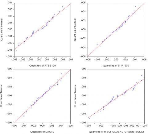
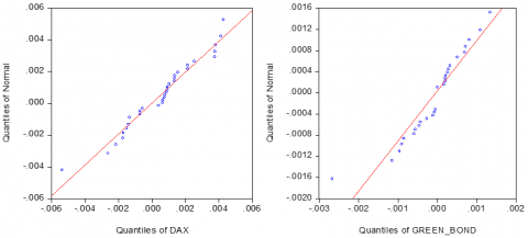
Table 1 reports the descriptive statistics of the monthly returns of the six assets with the Jarque–Bera (JB) normality test. The results indicate a substantial difference in variance, highlighting the relatively low volatility of green bond returns, in contrast with the higher variability observed for the MSCI Global Green Building index. According to the JB test, as well as the skewness and kurtosis values, the return series of all assets appear to be normally distributed, except green bonds. To strengthen this result, we complement the Jarque–Bera test with QQ-plots (see Appendix), which graphically confirm the normality of most return series and highlight some deviations in the case of green bonds.
Table 2 reports the correlation matrix of the return series. The results indicate that the MSCI Global Green Building Index is strongly and positively correlated with the developed stock indices, with coefficients ranging from 0.73 to 0.76. In contrast, green bonds exhibit much weaker correlations with stock indices, with coefficients between 0.10 and 0.33.
Table 1. Summary statistics of monthly returns
|
|
FTSE 100 |
S&P 500 |
CAC 40 |
DAX |
MSCI_G_G_B |
GREEN BONDS |
|
Mean |
0.0001 |
0.0004 |
0.0002 |
0.0005 |
-0.0002 |
-7.24E-05 |
|
Std. Dev. |
0.0015 |
0.0022 |
0.0022 |
0.0022 |
0.0022 |
0.0007 |
|
Skewness |
-0.1969 |
-0.4000 |
0.1100 |
-0.2992 |
0.0797 |
-1.2120 |
|
Kurtosis |
2.1394 |
2.4877 |
2.2358 |
3.1194 |
2.1318 |
6.3898 |
|
Jarque-Bera |
1.2315 |
1.2411 |
0.8696 |
0.5120 |
1.0714 |
23.8800 |
|
Prob |
0.5402 |
0.5376 |
0.6473 |
0.7741 |
0.5852 |
0.0000 |
Table 2. Correlation matrix of monthly returns
|
|
FTSE 100 |
S&P 500 |
CAC 40 |
DAX |
MSCI_G_G_B |
GREEN BONDS |
|
FTSE100 |
1.0000 |
|
|
|
|
|
|
S&P 500 |
0.5995 |
1.0000 |
|
|
|
|
|
CAC40 |
0.7689 |
0.7485 |
1.0000 |
|
|
|
|
DAX |
0.7642 |
0.8603 |
0.9164 |
1.0000 |
|
|
|
MSCI_G_G_B |
0.7652 |
0.7477 |
0.7366 |
0.7628 |
1.0000 |
|
|
GREEN BONDS |
0.1060 |
0.3320 |
0.1333 |
0.1654 |
0.1356 |
1.0000 |
3.1 Portfolio optimization
3.1.1 The Markowitz model
Modern portfolio analysis begins with pioneering research by Markowitz [15]. The portfolio selection model, first formulated by Markowitz, is called the mean-variance (MV) model. Markowitz's MV method is the classic paradigm in modern finance for allocating capital among risky assets. In this model, an efficient portfolio maximizes expected return for a given level of risk, or equivalently minimizes risk for a given level of return. The collection of such portfolios constitutes the efficient frontier.
The optimization problem can be expressed as:
$\operatorname{Min} \sigma_p^2=\sum_{i=1}^n \sum_{j=1}^n w_i w_j \sigma_{i j}$ (1)
Subject to:
$\begin{gathered}\sum_{i=1}^n w_i E\left(R_i\right)=E\left(R_p\right) \\ \sum_{i=1}^n w_i=1, w_i \geq 0\end{gathered}$ (2)
Or equivalently:
$\operatorname{Max} E\left(R_p\right)=\sum_{i=1}^n x_i E\left(R_i\right)$ (3)
Subject to:
$\sigma_p^2=\sum_{i=1}^n \sum_{j=1}^n w_i w_j \sigma_{i j}$ (4)
$\sum_{i=1}^n w_i=1, w_i \geq 0$ (5)
where,
n: is the number of different assets making up the portfolio
$\sigma_{i j}$: is the covariance between the returns of assets i and j
$w_i$: is the weight of each asset in the portfolio
$r_i$: is the average return of asset i
$\sigma_p^2$: the variance of the portfolio
R: is the desired average return of the portfolio.
Assumptions of the Markowitz Model
The model relies on two categories of assumptions:
3.1.2 Genetic algorithms (GA)
Genetic algorithms (GA) are a stochastic optimization technique developed by Holland [16] and based on the principles of Darwinian evolution, namely survival of the fittest and information exchange. In each generation, a new set of artificial creatures (encoded as strings) is constructed from the best elements of the previous generation. Although relying on randomness, these algorithms are not purely random [17]. The population-based approach is particularly beneficial in exploring optimal portfolio selection solutions. Genetic algorithms have been applied to a wide range of optimization problems and offer significant advantages in terms of methodology and performance. In recent years, there has been a growing use of genetic algorithms to solve multi-objective optimization problems, also known as evolutionary multi-objective optimization. The key characteristic of GAs is their global and multidirectional search, in which a population of potential solutions is maintained and evolved from generation to generation. Many studies have shown that GAs can efficiently find near-optimal solutions for combinatorial optimization problems, such as the work of Soleimani et al. [18], who demonstrated their reliability in real markets with many assets. The applications of GAs in finance have been booming and are now included in finance textbooks [19]. Similarly, Pereira [20] argued that GAs are a valid approach for many complex financial problems requiring robust optimization techniques.
Genetic Algorithms Principle. The main advantage of GAs is that it is not necessary to specify all details of a problem in advance. Candidate solutions are evaluated by an objective function, and an evolutionary procedure produces new ones. The idea is to combine good solutions to generate better ones, while introducing small perturbations (mutations) to maintain diversity and avoid premature convergence.
Genetic Algorithm Operators. The genetic algorithm starts randomly with a population of size ‘k’. Three genetic operations (selection, crossover, and mutation) are repeated for the elements of the population k to move to a second-generation k+1. Starting with the first genetic operation, selection aims to optimize the objective function by retaining the most relevant elements. Crossover is the main genetic operator. It operates on two parent chromosomes at a time and generates two new chromosomes by combining their characteristics. In the case of a weight selection problem, crossover plays the role of exchanging the weights of the securities making up the portfolio. There are several forms of crossover: one-point, two-point, multi-point, and uniform. Finally, mutation is a background operator that produces random changes in chromosomes. Mutation is used to maintain diversity in the population and to prevent premature convergence of solutions. While crossover generates new individuals that are distant from their parents in the search space, mutation introduces small perturbations to further explore the space.
The mathematical formulation of the objective function in a GA application. The evaluation is performed through an objective function, which depends on the specific problem and the optimization goal of the GA [21]. The objective is to determine the optimal proportions associated with each asset to maximize portfolio return and minimize risk. The mathematical model, which extends the Markowitz mean-variance approach, is presented as follows:
$\operatorname{Min} \delta_p^2(w)=\sum_{i=1}^n \sum_{j=1}^n w_i w_j \sigma_{i j}$ (6)
$\operatorname{Max} r_p(w)=\sum_{i=1}^n \mu_i w_i$ (7)
Under constraints: $\sum_{i=1}^n w_i=1$ and $w_i \geq 0, i=1, \ldots, n$
$\delta^2{ }_p$: Portfolio variance
$r_p$: return
$\sigma_{i j}$: the covariance between the returns of assets i and j
$w_i$: the weight of each asset in the portfolio
$\mu_i$: the average return on asset i
Normally, single-objective optimization aims to find a single global optimum solution. However, multi-objective optimization seeks to identify a set of Pareto optimal solutions, since it involves two or more conflicting objectives. In this study, the multi-objective portfolio optimization problem is formulated as follows:
$\operatorname{MinH}(w)=\delta^2{ }_p(w)-r_p(w)$ (8)
Under constraints: $\sum_{i=1}^n w_i=1$ and $w_i \geq 0, i=1, \ldots, n$
The fitness function. The fitness function is a key component of GA in solving optimization problems. In asset allocation, it must ensure a rational trade-off between risk reduction and return maximization. Thus, it can be designed as follows:
$\operatorname{MinH}(w)=\delta^2{ }_p(w)-r_p(w)$ (9)
The fitness function of each chromosome is the criterion that enables the GA to perform selection.
The Markowitz mean-variance (MV) model represents the classical analytical framework for portfolio optimization and provides the efficient frontier by minimizing risk for a given return or maximizing return for a given risk. However, the MV model relies on strong assumptions, such as return normality and the existence of closed-form analytical solutions, which may limit its application in complex or real-world environments. In contrast, genetic algorithms (GA) constitute a heuristic and flexible approach that can explore the solution space more broadly and efficiently. They are particularly well-suited for multi-objective problems, where the simultaneous minimization of risk and maximization of return naturally generate a set of Pareto-optimal portfolios rather than a single solution. Therefore, in this study, MV and GA are not presented as competing techniques but as complementary approaches: while MV provides a theoretical benchmark through the efficient frontier, GA enables the generation of alternative portfolios that may be better adapted to practical constraints and robustness checks. Finally, in this study, after applying the two optimization approaches (MV and GA), we compare the resulting optimal portfolios using three complementary methods: (i) the Sharpe ratio, which measures risk-adjusted performance; (ii) the Markowitz efficient frontier, which serves as an analytical benchmark; and (iii) the stochastic dominance (SD) criterion, which allows us to assess portfolio robustness beyond the mean–variance framework.
3.2 Portfolio selection
3.2.1 Reward-to-risk ratio
The main advantage of performance measures is that they allow the comparison of the results of several portfolios. We have chosen as a performance measure ‘reward-to-risk ratio’, λ [22]. Several authors have used this ratio to compare the performances of portfolios [23, 24]. This ratio is chosen for its popularity and its simple implementation. This ratio is calculated as follows.
$\lambda=\frac{\mathbf{R}_{\mathbf{i}} / \sigma_{\mathbf{i}}^2}{\mathbf{R}_{\mathbf{m}} / \sigma_{\mathbf{m}}^2}$, (10)
With
λ: reward-to-risk ratio,
$\mathbf{R}_{\mathbf{m}}$: Average return of the market portfolio m,
$\sigma_m^2$: The variance of the return of the market portfolio m.
We followed authors who used the stock index (e.g., S&P 500) to present the market portfolio [22]. The more this ratio increases, the more the portfolio performs.
3.2.2 Modern Portfolio Theory
Modern Portfolio Theory [15] provides the theoretical basis for portfolio selection. It shows that efficient portfolios maximize return for a given level of risk or minimize risk for a given return, and they are represented by the efficient frontier. In this study, we rely on this framework as a benchmark to compare the performance of the portfolios optimized through both the MV model and the genetic algorithm.
3.2.3 The stochastic dominance (SD) approach
The traditional Mean-Variance (MV) approach of Markowitz [15] consists of optimizing portfolios while maximizing the return for a given level of risk or minimizing the risk measured by the standard deviation for a given level of return. Indeed, several researchers use the MV approach in their empirical work in the evaluation of their portfolios. Despite the frequent use of this method, the latter has been criticized. Indeed, it is not sufficient for the comparison between two random variables since it is based only on two statistics, namely the mean and the variance. In addition, this method assumes the normality of returns, which is not always the case. The stochastic dominance (SD) approach, developed by Hadar and Russell [25] and others, manages to remedy the limitations left by the traditional MV approach. It has the advantage of being based on less restrictive assumptions. It can be applied even if the series of returns is not Gaussian. The SD determines the criteria for comparison between financial assets on the utility functions of investors (their preferences, their attitudes towards risk) and the statistical properties of the returns. It is more informative than the traditional approach because it uses all the information on the distribution in order to establish an adequate comparison. Several studies [24, 26] use the SD to compare the performance of portfolios.
Let F and G be two distribution functions (CDFs) of the two portfolios X and Y, and let f and g be the probability density functions of the two portfolios, respectively, defined on a common interval [a, b].
Let
$\mathrm{H} 0=\mathrm{h}$ et $H_j(n)=\int_a^n H_{j-1}(t) d t$ (11)
for h = f, g; H = F,G and j = 1,2,3. There are 3 orders of stochastic dominance: 1st order, 2nd order, and 3rd order dominance. Let the utility of X be denoted u(X).
First-order stochastic dominance (FSD) is based on less restrictive assumptions. Indeed, in this case, agents are not risk-averse, they always prefer to maximize their wealth.
X dominates Y according to the first order if:
X dominates Y according to the 2nd order (SSD) if:
X dominates Y according to the 3rd order (TSD) if:
Stochastic Dominance Test:
Stochastic dominance has two classes of tests:
Let two assets X and Y with their distribution functions $F$ and $G$, respectively, and for a grid of predetermined points n1, n2 ... nk, the DD statistic of order j, Tj (n) (j = 1, 2 et 3), is as follows:
$\widehat{T}_j(n)=\frac{\widehat{F}_j(n)-\widehat{G}_j(n)}{\sqrt{\widehat{V}_j(n)}}$ (12)
With
$\begin{gathered}\widehat{V}_j(n)=\widehat{V}_x^j(n)+\widehat{V}_y^j(n)-2 \widehat{V}_{x, y}^j(n), \\ \widehat{H}_j(n)=\frac{1}{N(j-1)!} \sum_{i=1}^N\left(n-h_i\right)_{+}^{j-1}, \\ \widehat{V}_H^j(n)=\frac{1}{N}\left[\frac{1}{N((j-1)!)^2} \sum_{i=1}^N\left(n-h_i\right)_{+}^{2(j-1)}-\widehat{H}_j(n)^2\right], \mathrm{H}=F, G \\ \text { et } \mathrm{h}=x, y, \\ \widehat{V}_{x, y}^j(n)=\frac{1}{N}\left[\frac{1}{N((j-1)!)^2} \sum_{i=1}^N\left(n-x_i\right)_{+}^{j-1}\left(n-y_i\right)_{+}^{j-1}-\right. \\ \left.\widehat{F}_j(n) \widehat{G}_j(n)\right] .\end{gathered}$
$F$ and $G$ were defined in (8) and $(n)_{+}=\max \{n, 0\}$.
It is not possible to empirically test the hypothesis H0 for the entire range of distributions. Indeed, we will test the null hypothesis for a preconceived finite number k of values n, $\left\{n_k, k=1,2 \ldots, k\right\}$. Thus, the appropriate choice of k for reasonably large samples is between 6 and 15 [27]. Following Wong et al. [29] and others, the choice of K grid points should have the same length as the two random samples {Xi} and {Yi}.
The hypotheses to be tested are as follows:
H0: $F_j\left(n_i\right)=G_j\left(n_i\right)$ for all $n, \mathrm{i}=1,2 \ldots, \mathrm{k}$,
HA: $F_j\left(n_i\right) \neq G_j\left(n_i\right)$ for some $n_i$,
HA1: $F_j\left(n_i\right) \leq F_j\left(n_i\right)$ for all $n_i, F_j\left(n_i\right)<G_j\left(n_i\right)$ for some $n_i$,
HA2: $F_j\left(n_i\right) \geq G_j\left(n_i\right)$ for all $a_i, F_j\left(n_i\right)>G_j\left(n_i\right)$ for some $n_i$,
Let the critical point that will allow us to control the probability of rejecting the null hypothesis be $M^k{ }_{\infty \alpha}$, with infinite degrees of freedom and α the significance threshold. We obtained it using the distribution of the ‘Studentized Maximum Modulus’ (SMM) tabulated by Stoline and Ury [30], following Bishop et al. [31].
We will adopt the following decision rules:
We note that in the above assumptions, HA is excluded from both HA1 and HA2, which means that if either HA1 or HA2 is accepted, it does not mean that HA is accepted. Accepting either H0 or HA implies that there are no SD relations and no arbitrage opportunity between these two portfolios, and neither of these two portfolios is preferred to the other. However, if HA1 or HA2 is accepted at first order, it shows that a P1 portfolio stochastically dominates a P2 portfolio at first order. In this situation, there is an arbitrage opportunity and, as a result, investors can maximize their expected wealth if they move from the dominated portfolio to the dominant one. On the other hand, if HA1 or HA2 is accepted according to the 2nd or 3rd order, we say that P1 stochastically dominates P2 at the 2nd or 3rd order. In this situation, an arbitrage opportunity does not exist, and the transition from one portfolio to another will only increase investors' expected utility, but not their expected wealth [29].
In this study, we focus on the impact of green assets, namely the MSCI Global Green Building Index and global green bonds, when integrated into investment portfolios. To this end, we construct three portfolio configurations:
Our analysis is conducted under two scenarios:
For both scenarios, we evaluate portfolio performance using the reward-to-risk ratio, the Markowitz efficient frontier, and the stochastic dominance approach.
4.1 Portfolio optimization
4.1.1 Asset allocation while minimizing risk
The weights reported in Table 3 indicate the percentage of an investor’s assets that should be allocated to each index at the optimized level when minimizing portfolio risk. This study employed the Excel Solver to compute the optimal weights that minimize risk for the three portfolios under consideration. For Portfolio P1, the expected return and risk were 3E-4 and 4.98E-6, respectively, with optimal weights of 41.289% for the S&P 500 and 58.71% for the FTSE 100. For Portfolio P2, the expected return and risk were 3E-4 and 4.93E-6, with weights of 75.335% for the S&P 500 and 24.665% for the MSCI Global Green Building Index. And for Portfolio P3, the expected return and risk were 3E-4 and 4.65E-6, with weights of 66.20% for the S&P 500 and 33.80% for green bonds. From Table 3, it can be observed that an investor seeking an efficient portfolio with minimal risk (i.e., a risk-averse investor) should allocate 24.665% of assets to the MSCI Global Green Building Index and 33.80% to green bonds to achieve an expected return of 3E-4. Overall, Table 3 highlights that including green investments in a portfolio composed of the main developed stock indices reduces overall risk. Moreover, the optimal allocation to green bonds (33.80%) is higher than that to the MSCI Global Green Building Index (24.665%), reinforcing their greater role in risk mitigation.
4.1.2 Asset allocation using genetic algorithms
The weights of different columns (Table 4) indicate what percentage of an investor’s assets should be allocated to the index in question at the optimized level when using genetic algorithms. For the P1 portfolio, the optimal weights were 0.6% for FTSE100, 19.39% for S&P500, 0.52% for CAC40, and 79.56% for DAX, with the expected return and risk being 5.3E-4 and 4.55E-6, respectively. For the P2 portfolio, the optimal weights were 3.82% for FTSE100, 14.15% for S&P500, 5.7% for CAC40, 72.06% for DAX, and 4.36% for MSCI global green building, the expected return and risk being 5.3E-4 and 4.55E-6, respectively. Concerning the P3 portfolio, the optimal weights were 18.35% for S&P500, 4.17% for CAC40, 69.63% for DAX, and 7.95% for green bonds, with the expected return and risk being 4.73E-4 and 3.9E-6, respectively. Based on the GA method, an investor seeking to maximize return while minimizing risk should allocate 4.36% of assets to the MSCI global green building and 7.95% to green bonds. Table 4 shows that including green investments in a portfolio composed of major developed stock indices lowers overall risk, and that the optimal weight for green bonds is higher than that for the MSCI global green building.
From Tables 3 and 4, we note that the optimal weights of green assets differ depending on the investor’s attitude towards risk. Indeed, the optimal weights are greater when the investor is risk-averse.
Table 3. Optimization of the 3 portfolios while minimizing the variance
|
Portfolios |
P1 |
P2 |
P3 |
|
FTSE100 |
58.71% |
0 |
0 |
|
S&P500 |
41.289% |
75.335% |
66.20% |
|
CAC40 |
0 |
0 |
0 |
|
DAX |
0 |
0 |
0 |
|
MSCI_G_G_B |
- |
24.665% |
- |
|
GREEN BONDS |
- |
- |
33.80% |
|
RETURN |
3E-4 |
3E-4 |
3E-4 |
|
VARIANCE |
4.98E-6 |
4.93E-6 |
4.65E-6 |
Table 4. Optimization of the 3 portfolios using genetic algorithms (GA)
|
Portfolios |
P1 |
P2 |
P3 |
|
FTSE100 |
0.63% |
3.82% |
0 |
|
S&P500 |
19.39% |
14.15% |
18.35% |
|
CAC40 |
0.52% |
5.7% |
4.17% |
|
DAX |
79.56% |
72.06% |
69.63% |
|
MSCI_G_G_B |
- |
4.36% |
- |
|
GREEN BONDS |
- |
- |
7.95% |
|
RETURN |
5.3E-4 |
4.69E-4 |
4.73E-4 |
|
VARIANCE |
4.55E-6 |
4.34E-6 |
3.90-6 |
4.2 Portfolio selection
4.2.1 Performance measurement using the reward-to-risk ratio
From the results displayed in Table 5, we notice that the performance of the P2 and P3 portfolios, which include green investments, is superior to that of P1. In particular, the reward-to-risk ratio improves when green assets are incorporated compared to the traditional portfolio. These findings confirm the positive role of green assets in enhancing portfolio diversification by reducing variance.
Table 5. Performance measurement using reward to risk ratio for the 3 portfolios optimized by minimizing variance
|
|
P1 |
P2 |
P3 |
|
λ: reward-to-risk ratio |
0.688 |
0.695 |
0.737 |
Comparing the reward-to-risk ratio values for the three portfolios optimized by genetic algorithms, Table 6 reveals that the ratio increases for the portfolio including green bonds compared to the traditional portfolio. In contrast, the P2 portfolio, which incorporates the MSCI Global Green Building index, shows a lower performance ratio than P1. This result emphasizes that portfolios including green bonds outperform the benchmark portfolio.
Table 6. Performance measurement using reward to risk ratio for the 3 portfolios optimized by GA
|
|
P1 |
P2 |
P3 |
|
λ: reward-to-risk ratio |
1.331 |
1.235 |
1.386 |
4.2.2 Efficient frontier
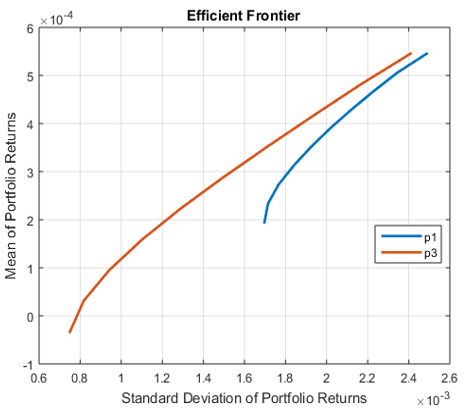
Figure 1 plots two efficient frontiers. The brown frontier represents the efficient frontier that includes the MSCI Global Green Building Index (portfolio P2), while the blue frontier corresponds to the efficient frontier without green assets (portfolio P1). It can be observed that portfolio P2 shifts the frontier upward, clearly dominating the other curve. This indicates that, for the same level of risk, portfolios with green assets provide higher returns. The same interpretation applies to green bonds (Figure 2).
Figure 1. Efficient frontiers’ comparison for two portfolios P1 and P2
Figure 2. Efficient frontiers’ comparison for two portfolios P1 and P3
4.2.3 Stochastic dominance (SD)
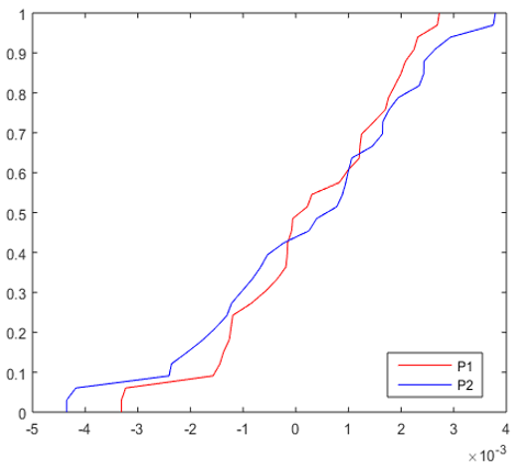
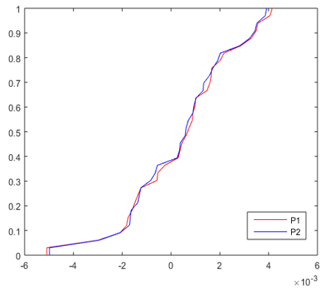
SD for the 1st scenario. After optimizing the portfolios using two methods, namely the Markowitz approach (minimizing variance for a given level of return) and the genetic algorithm method, we proceed to apply the stochastic dominance (SD) approach to further evaluate the relative performance of the optimized portfolios under each scenario. SD for the first scenario. From Figures 3 and 4, we observe that the empirical distribution functions of portfolios P1 and P2, as well as those of P1 and P3, intersect. This implies that it is very likely that there is no first-order stochastic dominance between the portfolios. In other words, there is no clear arbitrage opportunity between a portfolio without green assets and one that includes green assets. The same interpretation applies to the second scenario (Figures 5 and 6).
Figure 3. Plot of the cumulative distribution functions of the two optimal portfolios P1 and P2
Figure 4. Plot of the cumulative distribution functions of the two optimal portfolios P1 and P3
Figure 5. Plot of the cumulative distribution functions of the two optimal portfolios P1 and P2
Figure 6. Plot of the cumulative distribution functions of the two optimal portfolios P1 and P3
Table 7 reveals that the portfolio including green bonds (P3) dominates the traditional portfolio (P1) according to the second and third-order stochastic dominance criteria. However, the portfolio with MSCI Global Green Building (P2) and the traditional portfolio (P1) do not dominate each other. This result indicates that risk-averse investors would prefer to include green bonds in their portfolios in order to maximize their expected utility, while they remain indifferent between holding an optimal conventional portfolio with or without MSCI Global Green Building. The same results are observed for the second scenario (Table 8). Our findings are consistent with Han and Li [14], who also highlight the beneficial role of green bonds in portfolio diversification. This evidence can therefore be of practical use to portfolio managers seeking alternative assets to reduce portfolio risk and improve diversification.
Table 7. Stochastic dominance between P1, P2 and P3
|
|
P2 |
P3 |
|
P1 |
ND |
$\prec^{2,3}$ |
SD for the 2nd scenario.
Table 8. Stochastic dominance between P1, P2 and P3
|
|
P2 |
P3 |
|
P1 |
ND |
$\prec^{2,3}$ |
This study provides new insights into the integration of green assets, specifically green bonds and the MSCI Global Green Building Index, into optimal portfolio construction. The results demonstrate that incorporating green bonds consistently reduces portfolio risk and improves diversification, while the green index delivers more modest benefits. Importantly, second and third-order stochastic dominance confirm that portfolios, including green bonds, are preferred by risk-averse investors, whereas portfolios with the green index remain equivalent to traditional ones. These findings have significant implications for portfolio managers and investors concerned with sustainability, as they highlight that green bonds can simultaneously enhance financial performance and support environmental objectives. However, the study has certain limitations. First, the analysis is restricted to a limited set of indices and a specific time horizon, which may affect the generalizability of the results. Second, only two optimization techniques were applied: mean-variance and genetic algorithms, while other standard approaches, such as CVaR optimization or NSGA-II, could provide additional insights. Future research could therefore extend the analysis by considering a broader range of green assets [32], applying alternative optimization methods, and examining different time periods to test the robustness of the results.
|
MSCI_G_G_B |
The MSCI Global Green Building Index |
|
MV |
The Markowitz mean–variance |
|
GA |
Genetic Algorithms |
|
SD |
Stochastic dominance |
[1] Solnik, B.H., McLeavey, D. (2009). Global Investments. Pearson Education.
[2] Abidin, P.E. (2004). Sweetpotato Breeding for Northeastern Uganda: Farmer Varieties, Farmer-Participatory Selection, and Stability of Performance. ProQuest Dissertations & Theses, Wageningen University and Research.
[3] Sharpe, S.A. (1994). Financial market imperfections, firm leverage, and the cyclicality of employment. The American Economic Review, 84(4): 1060-1074.
[4] Ameur, H.B., Ftiti, Z., Louhichi, W., Yousfi, M. (2024). Do green investments improve portfolio diversification? Evidence from mean conditional value-at-risk optimization. International Review of Financial Analysis, 94: 103255. https://doi.org/10.1016/j.irfa.2024.103255
[5] Xie, Q., Wang, D., Bai, Q. (2024). “Cooperation” or “competition”: Digital finance enables green technology innovation—a new assessment from dynamic spatial spillover perspectives. International Review of Economics & Finance, 93: 587-601. https://doi.org/10.1016/j.iref.2024.04.040
[6] Viviani, J.L., Fall, M., Revelli, C. (2019). The effects of socially responsible dimensions on risk dynamics and risk predictability: A value-at-risk perspective. Management International, 23(3): 141-157. https://doi.org/10.7202/1062215ar
[7] Ren, B., Lucey, B. (2022). A clean, green haven?—Examining the relationship between clean energy, clean and dirty cryptocurrencies. Energy Economics, 109: 105951. https://doi.org/10.1016/j.eneco.2022.105951
[8] Naeem, M.A., Karim, S. (2021). Tail dependence between Bitcoin and green financial assets. Economics Letters, 208: 110068. https://doi.org/10.1016/j.econlet.2021.110068
[9] Akhtaruzzaman, M., Banerjee, A.K., Boubaker, S., Moussa, F. (2023). Does green improve portfolio optimization? Energy Economics, 124: 106831. https://doi.org/10.1016/j.eneco.2023.106831
[10] Naeem, M.A., Nguyen, T.T.H., Nepal, R., Ngo, Q.T., Taghizadeh–Hesary, F. (2021). Asymmetric relationship between green bonds and commodities: Evidence from extreme quantile approach. Finance Research Letters, 43: 101983. https://doi.org/10.1016/j.frl.2021.101983
[11] Reboredo, J.C., Ugolini, A. (2020). Price connectedness between green bond and financial markets. Economic Modeling, 88: 25-38. https://doi.org/10.1016/j.econmod.2019.09.004
[12] Kanamura, T. (2020). Are green bonds environmentally friendly and good-performing assets? Energy Economics, 88: 104767. https://doi.org/10.1016/j.eneco.2020.104767
[13] Pham, L., Nguyen, C.P. (2021). Asymmetric tail dependence between green bonds and other asset classes. Global Finance Journal, 50: 100669. https://doi.org/10.1016/j.gfj.2021.100669
[14] Han, Y., Li, J. (2022). Should investors include green bonds in their portfolios? Evidence for the USA and Europe. International Review of Financial Analysis, 80: 101998. https://doi.org/10.1016/j.irfa.2021.101998
[15] Markowitz, H. (1952) Portfolio selection. Journal of Finance, 7: 77-91. https://doi.org/10.1111/j.1540-6261.1952.tb01525.x
[16] Holland, J.H. (1975). Adaptation in Natural and Artificial Systems: An Introductory Analysis with Applications to Biology, Control, and Artificial Intelligence. University of Michigan Press, Michigan.
[17] Christophe, J. (1995). Glucagon receptors: From genetic structure and expression to effector coupling and biological responses. Biochimica et Biophysica Acta (BBA)-Reviews on Biomembranes, 1241(1): 45-57. https://doi.org/10.1016/0304-4157(94)00015-6
[18] Soleimani, H., Golmakani, H.R., Alimi, M.H. (2009). Markowitz-based portfolio selection with minimum transaction lots, cardinality constraints and regarding sector capitalization using a genetic algorithm. Expert Systems with Applications, 36(3): 5058-5063. https://doi.org/10.1016/j.eswa.2008.06.007
[19] Yıldızoğlu, M., Vallée, T. (2003). Présentation des algorithmes génétiques et de leurs applications en économie. Revue d'éConomie Politique, 114(6): 711-745.
[20] Pereira, R. (2000). Genetic algorithm optimization for finance and investments. MPRA Paper 8610, University Library of Munich, Germany.
[21] Petridis, V., Kazarlis, S., Bakirtzis, A. (1998). Varying fitness functions in genetic algorithm constrained optimization: The cutting stock and unit commitment problems. IEEE Transactions on Systems, Man, and Cybernetics, Part B (Cybernetics), 28(5): 629-640. https://doi.org/10.1109/3477.718514
[22] Hillier, D., Draper, P., Faff, R. (2006). Do precious metals shine? An investment perspective. Financial Analysts Journal, 62(2): 98-106. https://doi.org/10.2469/faj.v62.n2.4085
[23] Van Hoang, T.H. (2010). The gold market at the paris stock exchange: A risk-return analysis 1950-2003/der goldmarkt an der pariser börse: Eine rendite-risiko-analyse 1950-2003. Historical Social Research/Historische Sozialforschung, 389-411.
[24] Lean, H.H., Wong, W.K. (2015). Is gold good for portfolio diversification? A stochastic dominance analysis of the Paris stock exchange. International Review of Financial Analysis, 42: 98-108. https://doi.org/10.1016/j.irfa.2014.11.020
[25] Hadar, J., Russell, W.R. (1969). Rules for ordering uncertain prospects. American Economic Review, 59(1): 25-34.
[26] Abid, F., Leung, P.L., Mroua, M., Wong, W.K. (2014). International diversification versus domestic diversification: Mean-variance portfolio optimization and stochastic dominance approaches. Journal of Risk and Financial Management, 7(2): 45-66. https://doi.org/10.3390/jrfm7020045
[27] Barrett, G.F., Donald, S.G. (2003). Consistent tests for stochastic dominance. Econometrica, 71(1): 71-104. https://doi.org/10.1111/1468-0262.00390
[28] Davidson, R., Duclos, J.Y. (2000). Statistical inference for stochastic dominance and for the measurement of poverty and inequality. Econometrica, 68(6): 1435-1464. https://doi.org/10.1111/1468-0262.00167
[29] Wong, W.K., Phoon, K.F., Lean, H.H. (2008). Stochastic dominance analysis of Asian hedge funds. Pacific-Basin Finance Journal, 16(3): 204-223. https://doi.org/10.1016/j.pacfin.2007.07.001
[30] Stoline, M.R., Ury, H.K. (1979). Tables of the studentized maximum modulus distribution and an application to multiple comparisons among means. Technometrics, 21: 87-93. https://doi.org/10.1080/00401706.1979.10489726
[31] Bishop, J.A., Formby, J.P., Thistle, P.D. (1992). Convergence of the South and non-south income distributions, 1969-1979. The American Economic Review, 82(1): 262-272.
[32] Belkhir, N., Boujelbène, M., Mezghani, T. (2025). Exploring asymmetric effects of uncertainties on the time-varying nexus of green sukuk, clean and dirty energy markets under various market conditions. Journal of Islamic Accounting and Business Research. https://doi.org/10.1108/JIABR-09-2024-0336