Sunsanee Maneechot![]()
© 2025 The author. This article is published by IIETA and is licensed under the CC BY 4.0 license (http://creativecommons.org/licenses/by/4.0/).
OPEN ACCESS
Nakhon Ratchasima City, Thailand functions as the central hub of economic and social development in Nakhon Ratchasima City, reflected in the rapid expansion of urban settlements and built-up areas. The present study was conducted with three primary objectives: (1) to analyze land use and land cover (LULC) changes, (2) to examine spatial distribution trends of land surface temperature (LST), and (3) to identify abnormally high- and low-temperature zones through the Getis-Ord Gi* spatial statistics technique, focusing on the period 2014–2024. Satellite images acquired from Landsat 8 (OLI/TIR) and Landsat 9 (OLI-2/TIRS-2) were employed as the dataset. LULC classification for three selected years was performed using the Support Vector Machine (SVM) algorithm. Subsequently, LST was retrieved for each time period, and spatial hot and cold spots were examined using the Getis-Ord Gi* method. The results underscore the direct relationship between land use dynamics and thermal variability. In particular, the expansion of urban areas substantially contributed to the proliferation of hot spots, whereas forest ecosystems and aquatic environments mitigated localized heating. Additionally, the study identifies potential “reverse-UHI” conditions in post-harvest croplands, offering new insights into Thailand’s urban thermal environment. These findings provide implications for sustainable urban planning and green space management.
Getis-Ord Gi* method, hotspots analysis, land surface temperature, land use and land cover, support vector machine algorithm
Urbanization has emerged as one of the pressing phenomena influencing land use and environmental conditions. Rapid population growth, migration from rural to urban centers, and the continuous demand for economic expansion have resulted in dramatic transformations of land use and land cover (LULC) [1, 2]. Such changes are particularly evident in developing countries, where urban growth frequently outpaces sustainable planning frameworks. As agricultural lands and natural ecosystems are converted into built-up environments, cities become increasingly vulnerable to the effects of climate variability, especially the intensification of surface heating. The interplay between LULC dynamics and land surface temperature (LST) has therefore become a critical subject of contemporary urban environmental studies, with wide-ranging implications for climate adaptation, ecological sustainability, and public health [3, 4]. LST represents a key parameter in the study of urban climate as it directly reflects the thermal characteristics of the Earth’s surface. Its variations are driven by multiple physical factors, including topography, vegetation distribution, and land use composition within urban areas [5, 6]. Vegetated areas moderate LST through evapotranspiration processes, which release moisture into the atmosphere and cool surface temperatures. Water bodies provide another cooling mechanism by reflecting solar radiation and facilitating energy exchange between land and atmosphere. In contrast, impervious surfaces such as asphalt, concrete, and rooftops absorb and retain large amounts of heat [7-10]. The differential heating effects of LULC types highlight the necessity of understanding spatial variations in LST as a foundation for effective urban climate resilience strategies.
In recent decades, geospatial technologies—particularly remote sensing (RS) and geographic information systems (GIS)—have revolutionized the study of LULC and LST dynamics. Multi-temporal satellite imagery has enabled researchers to monitor long-term changes in urban environments and evaluate their impacts on thermal conditions [9, 11-14]. Beyond simple trend analysis, spatial statistics have further advanced the detection of thermal anomalies. The Getis-Ord Gi* statistic, in particular, has been widely applied to identify hot spots (areas of significantly high temperatures) and cold spots (areas of significantly low temperatures) [8, 15, 16]. By calculating Z-scores that compare local values against global averages, this technique provides robust insights into the clustering of heat and cooling zones. Consequently, it serves as a powerful tool for identifying vulnerable areas within cities, guiding urban planners in developing strategies to mitigate heat stress and enhance environmental sustainability [17].
Nakhon Ratchasima City presents a compelling case study. As the principal urban center of Nakhon Ratchasima City and one of the largest cities in northeastern Thailand, it functions as a regional hub in governance, healthcare, education, commerce, industry, and tourism [18]. The district’s strategic location as a transportation nexus—integrating highways, railways, and the planned high-speed rail system—has further reinforced its role as a growth pole for the region. Population statistics underscore this trend, with the number of residents increasing from 448,725 in 2013 to 468,506 in 2023, reflecting an annual growth rate of 0.65% [19]. The expansion of population and infrastructure has inevitably accelerated land use transformations, with natural and agricultural areas increasingly converted into built-up settlements and industrial zones. These dynamics raise concerns about the thermal implications of urban expansion and the city’s vulnerability to heat accumulation.
Despite the availability of studies on LULC change, LST patterns, and urban heat phenomena, limited research has comprehensively integrated these components in the context of Nakhon Ratchasima City. Previous works have often focused either on land use transitions or on surface temperature dynamics in isolation. Very few studies have employed advanced spatial statistical approaches, such as the Getis-Ord Gi* method, to simultaneously analyze how land use changes drive thermal anomalies at the urban scale. This research gap limits our ability to fully understand the direct linkages between urban expansion, LST variability, and the clustering of heat and cooling zones in regional cities of Thailand. To address this gap, the present study investigates the interplay between LULC changes and LST variability in Nakhon Ratchasima City over a ten-year period (2014–2024). Using Landsat 8 and Landsat 9 imagery, combined with the Support Vector Machine (SVM) classification method, the research analyzes multi-temporal LULC patterns with high accuracy. LST values are derived for three selected years and further analyzed using the Getis-Ord Gi* technique to identify statistically significant hot and cold spots. Unlike many existing studies that examine only a single dimension of urban climate, this research adopts an integrative framework by linking land use dynamics, thermal variations, and spatial clustering analysis. In particular, this study introduces a novel perspective by identifying spatially contrasting heat behaviors across urban and agricultural interfaces, emphasizing the potential occurrence of “reverse-UHI” conditions—where certain post-harvest croplands exhibit higher surface temperatures than urban cores. Such thermal inversions have been rarely documented in Thailand. By integrating LULC change detection, satellite-derived LST, and spatial hotspot analysis, the research provides new empirical evidence that deepens understanding of Thailand’s urban thermal environment and informs sustainable land-use and climate-adaptation planning.
2.1 Study area
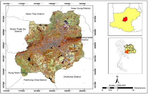
The study was conducted in Nakhon Ratchasima City, one of the 32 districts of Nakhon Ratchasima Province, located in northeastern Thailand. The district covers an area of approximately 755.60 km2 and lies between 14°47′N to 15°08′N latitude and 101°56′E to 102°14′E longitude. The elevation ranges from 200 to 250 meters above mean sea level. Geographically, the district is situated in the central part of the province. The dominant landforms consist of gently undulating terrain, with deeper undulating hills appearing near the foothill zones. The Lam Takhong River, a principal tributary of the Mun River, flows through the northern part of the city, playing a vital role in the district’s hydrological system. The spatial extent of the study area is illustrated in Figure 1.
Figure 1. Map of Nakhon Ratchasima City, Thailand
2.2 Data collection
Satellite imagery was collected from Landsat 8 (Operational Land Imager – OLI and Thermal Infrared Sensor – TIRS) and Landsat 9 (OLI-2/TIRS-2) for three time periods: 2014, 2019, and 2024. To account for seasonal variability, datasets were selected for both the winter and summer seasons in each year. All imagery was acquired from the United States Geological Survey (USGS) EarthExplorer platform (https://earthexplorer.usgs.gov/). The details of the satellite imagery used in this study are presented in Table 1.
Table 1. Landsat satellite imagery data used in the study
|
Landsat |
Path/Row |
Date |
Seasons |
|
Landsat 8 OLI/TIRS |
128/50 |
26 Jan 2014 26 Nov 2014 12 Dec 2014 |
Winter |
|
11 Feb 2014 27 Feb 2014 31 Mar 2014 |
Summer |
||
|
Landsat 8 OLI/TIRS |
128/50 |
24 Jan 2019 8 Nov 2019 10 Dec 2019 |
Winter |
|
9 Feb 2019 13 Mar 2019 30 Apr 2019 |
Summer |
||
|
Landsat 9 OLI-2 /TIRS-2 |
128/50 |
15 Feb 2024 18 Mar 2024 |
Summer |
|
Landsat 8 OLI/TIRS |
6 Jan 2024 23 Dec 2024 |
Winter |
|
|
27 Apr 2024 |
Summer |
2.3 Image pre-processing
2.3.1 Conversion of DN to spectral radiance
The first step of radiometric calibration involved the transformation of digital numbers (DN) into spectral radiance, using the radiometric rescaling factors provided in the Landsat metadata file. The conversion was performed using Eq. (1):
$\mathrm{L}_\lambda=\mathrm{M}_{\mathrm{L}} \mathrm{Q}_{\mathrm{cal}}+\mathrm{A}_{\mathrm{L}}$ (1)
where,
Lλ = spectral radiance (Watts/(m²·sr·μm))
ML = radiance multiplicative scaling factor for the band (from metadata)
Qcal = quantized calibrated pixel value (DN)
AL = radiance additive scaling factor for the band (from metadata)
2.3.2 Conversion of spectral radiance to TOA reflectance
The next step involved the conversion of spectral radiance into top-of-atmosphere (TOA) reflectance, which normalizes the radiance values by accounting for solar irradiance and the solar zenith angle. This correction enables comparison of reflectance values across different dates and acquisition conditions. The conversion was performed using Eqs. (2) and (3):
$\rho \lambda^{\prime}=\mathrm{M}_\rho \mathrm{Q}_{\mathrm{cal}}+\mathrm{A}_\rho$ (2)
where,
ρλ′ = TOA planetary reflectance without correction for solar angle
Mρ = reflectance multiplicative scaling factor for the band (from metadata)
Qcal = quantized calibrated pixel value (DN)
Aρ = reflectance additive scaling factor for the band (from metadata)
$\rho \lambda=\frac{\rho \lambda^{\prime}}{\cos \left(\theta_{\mathrm{S} Z}\right)}=\frac{\rho \lambda^{\prime}}{\sin \left(\theta_{\mathrm{SE}}\right)}$ (3)
where,
ρλ′ = TOA planetary reflectance without correction for solar angle
$\theta_{\mathrm{SE}}$ =solar elevation angle (in degrees, obtained from metadata)
$\theta_{\mathrm{SZ}}$ = solar zenith angle (in degrees); $\theta_{\mathrm{SZ}}$ = 90๐ - $\theta_{\mathrm{SE}}$
2.4 Land use and land cover (LULC) classification
LULC classification was performed using Landsat 8 (OLI) and Landsat 9 (OLI-2) images for three time periods: 2014, 2019, and 2024. False-color composite images (RGB: 4-5-3) were generated to enhance visual interpretation. A total of 182 training samples were collected to represent four major land use categories: (i) agricultural land, (ii) built-up and settlement areas, (iii) water bodies, and (iv) forest areas. A stratified random sampling approach was applied to ensure adequate spatial representation of each class across the 755 km² study area. Training and validation samples were interpreted and verified using high-resolution imagery from Google Earth and available field observations.
SVM algorithm was employed for image classification due to its strong capability in handling nonlinear and heterogeneous data distributions in complex urban–rural environments. The Radial Basis Function (RBF) kernel was selected, as it effectively separates mixed land-cover types by maximizing the margin between class boundaries. Parameter tuning for the penalty parameter (C) and kernel width (γ) was performed through an iterative grid search to optimize classification accuracy while preventing overfitting.
The classification results were validated against high-resolution satellite images from Google Earth. A total of 59 independent validation points were used for accuracy assessment through random sampling. Classification performance was evaluated using an error matrix and the Kappa coefficient [20], which measures the degree of agreement between the classified and reference data beyond chance. The results indicated that all classified maps achieved high overall accuracy (> 85%) and substantial agreement (Kappa > 0.85), confirming the reliability of the classification for subsequent spatial analysis.
2.5 Land surface temperature (LST)
LST was calculated from the thermal infrared bands of Landsat 8 (TIRS Band 10) and Landsat 9 (TIRS-2 Band 10) for the years 2014, 2019, and 2024. The computation followed the radiative transfer method [21], which converts thermal radiance into brightness temperature and subsequently adjusts for land surface emissivity (LSE). The general formula used is presented in Eq. (4):
$\mathrm{LST}=\frac{\mathrm{T}_{\mathrm{B}}}{1+\left(\lambda \times \mathrm{T}_{\mathrm{B}} / \rho\right) \ln \varepsilon}$ (4)
where,
LST = Land Surface Temperature
TB = at-satellite brightness temperature (Kelvin)
$\lambda$ = wave length
ρ = h × c/σ (1.438 × 10⁻² m K) = 14388 µm K
h = Planck’s constant (6.626 × 10⁻³⁴ J/s)
c = velocity of light (2.998 × 10⁸ m/s)
σ = Boltzmann constant (1.38 × 10⁻²³ J/K)
$\varepsilon$ = land surface emissivity
2.5.1 Brightness temperature (TB)
TB was derived from the thermal infrared band (Band 10) of Landsat 8 and Landsat 9 imagery. The process involved converting the DN values into spectral radiance, followed by the estimation of at-satellite brightness temperature. This step allows for the initial assessment of surface thermal conditions prior to emissivity correction. The calculation of TB was performed using Eq. (5):
$\mathrm{T}_{\mathrm{B}}=\frac{\mathrm{K}_2}{\ln \left(\frac{\mathrm{~K}_1}{\mathrm{~L}_\lambda}+1\right)}-273.15$ (5)
where,
TB = at-satellite brightness temperature (Kelvin)
K1 and K2 = calibration constants specific to the thermal infrared sensor (provided in metadata)
Lλ = spectral radiance (Watts/(m²·sr·µm))
2.5.2 Land surface emissivity (LSE)
LSE was estimated to correct TB values for surface thermal properties. LSE represents the efficiency of the Earth’s surface in emitting thermal radiation and is influenced by land cover characteristics, particularly vegetation fraction. In this study, emissivity was derived from the proportion of vegetation cover using the method proposed by Jesus and Santana [22]. The calculation was based on Eq. (6):
$\varepsilon=0.004 \times \mathrm{Pv}+0.986$ (6)
where,
ε = land surface emissivity
Pv = proportion of vegetation, derived from NDVI
2.5.3 Normalized difference vegetation index (NDVI)
The Normalized Difference Vegetation Index (NDVI) was employed to estimate vegetation cover and to support the calculation of LSE. NDVI represents the ratio of the difference between near-infrared (NIR) reflectance and red band reflectance to their sum, effectively distinguishing vegetated surfaces from bare soil and built-up areas. This index is widely used as a proxy for vegetation density and health [23]. NDVI was calculated using Eq. (7):
$\mathrm{NDVI}=\frac{\mathrm{NIR}-\mathrm{RED}}{\mathrm{NIR}+\mathrm{RED}}$ (7)
where,
NIR = reflectance in the near-infrared band
RED = reflectance in the red band
NDVI values range from –1 to +1. Higher values (close to +1) indicate dense and healthy vegetation, whereas lower values (close to 0 or negative) represent bare soil, impervious surfaces, or water bodies. The NDVI-derived vegetation proportion was subsequently used to refine emissivity estimates and improve the accuracy of LST retrieval.
2.5.4 Proportion of vegetation (Pv)
The proportion of vegetation (Pv) was calculated to represent the fractional vegetation cover within each pixel. PV is derived from NDVI values and is essential for estimating LSE. It provides a quantitative measure of vegetation density ranging from 0 (bare soil or impervious surface) to 1 (full vegetation cover). The calculation was performed using Eq. (8):
$\mathrm{Pv}=\left(\frac{\mathrm{NDVI}^{-} \mathrm{NDVI}_{\min }}{\mathrm{NDVI}_{\max }-\mathrm{NDVI}_{\min }}\right)^2$ (8)
where,
NDVImin = minimum NDVI value in the scene
NDVImax = maximum NDVI value in the scene
2.5.5 Validation of land surface temperature (LST)
To ensure the reliability of the retrieved LST, a validation procedure was conducted by comparing the satellite-derived LST values with ground-based temperature records. Surface air temperature data were obtained from the Nakhon Ratchasima Meteorological Station, operated by the Lower Northeastern Meteorological Center, for the same acquisition dates as the Landsat imagery. The degree of agreement between satellite-derived LST and ground-based observations was assessed using the coefficient of determination (R2). The R2 value ranges between – 1 and + 1, where values approaching +1 indicate a strong positive correlation and thus higher reliability of the satellite-derived LST. This validation step provides confidence in the accuracy of the RS–based thermal estimations used in this study.
2.6 Hot spot and cold spot analysis
The identification of anomalously high or low surface temperatures was carried out using the Getis-Ord Gi* spatial statistic. This method is widely applied to detect statistically significant spatial clustering of high values (Hot Spots) and low values (Cold Spots) within a study area. The analysis produces two key indicators: the z-score, which measures the statistical significance of clustering, and the p-value, which determines the probability level of such clustering being due to random chance.
In this study, the Gi* statistic was implemented using a fixed-distance band spatial weights matrix with a threshold of 1,000 m., determined from the average nearest-neighbor distance among sample pixels. This distance ensured that each feature had sufficient spatial neighbors to produce stable local statistics. To verify robustness, a sensitivity test using k-nearest neighbors (k = 8) was also conducted, yielding similar spatial clustering patterns.
To minimize bias from multiple significance testing, the results were adjusted using the False Discovery Rate (FDR) correction method. Only clusters with z-scores exceeding +1.96 (p < 0.05) or below −1.96 (p < 0.05) after FDR adjustment were interpreted as statistically significant Hot Spots or Cold Spots, respectively. The Gi* statistic was calculated using Eq. (9):
$G_i^*=\frac{\sum_{j=1}^n \omega_{i j} x_j-\bar{x} \sum_{j=1}^n \omega_{i j}}{s \sqrt{\frac{n \sum_{j=1}^n \omega_{i j}^2-\left(\sum_{j=1}^n \omega_{i j}\right)^2}{n-1}}}$ (9)
where,
$G_i^*$ = Getis-Ord Gi* statistic for location iii
$x_j$ = attribute value at location jjj
$\omega_{i j}$ = spatial weight between location iii and jjj
N = total number of features
$\bar{x}$ = mean of all attribute values
S = standard deviation of all attribute values
$S \sqrt{\frac{\sum_{j=1}^n x_j}{n}-(\bar{x})^2}$
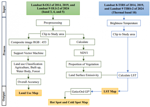
The evaluation of hot spots and cold spots was based on statistical confidence levels, which indicate the degree of significance in spatial clustering patterns. These confidence levels are directly associated with the p-value and z-score, providing a quantitative basis for distinguishing statistically significant hot and cold spots from random spatial variation [24]. In this study, three levels of statistical confidence were adopted, as shown in Table 2. The methodological framework and analytical steps of this study are summarized in the flowchart shown in Figure 2.
Figure 2. Flowchart of the methodology
Table 2. Hot-spot classification by applying Getis-Ord Gi*
|
Gi* Hot-Spot Classes |
Confidence Levels |
Probability (Gi* P-Value) |
Standard Deviation (Gi* Z-Score) |
|
Cold-spot99 (LEVEL-3) |
99% |
<0.01 |
<-2.58 |
|
Cold-spot95 (LEVEL-2) |
95% |
<0.05 |
<-1.96 |
|
Cold-spot90 (LEVEL-1) |
90% |
<0.10 |
<-1.65 |
|
Other areas |
Not Significant |
0 |
-1.65 < z-score < 1.65 |
|
Hot-spot90 (LEVEL-1) |
90% |
<0.10 |
>1.65 |
|
Hot-spot95 (LEVEL-2) |
95% |
<0.05 |
>1.96 |
|
Hot-spot99 (LEVEL-3) |
99% |
<0.01 |
>2.58 |
2.7 Statistical validation of LST variation by land use and season
To statistically verify the influence of LULC and season on LST, a two-way Analysis of Variance (ANOVA) was conducted using SPSS software. The independent factors included LULC class (built-up, agriculture, forest, and water body) and season (winter and summer), while the dependent variable was the mean LST extracted from Landsat-derived thermal bands. The test was designed to determine whether significant differences in LST exist among LULC types, between seasons, and in the interaction between these two factors. The analysis was performed for the combined dataset representing all study years (2014, 2019, and 2024), with each class containing three replicated sampling units per year and season.
3.1 Land use and land cover (LULC) changes in Nakhon Ratchasima City (2014–2024)
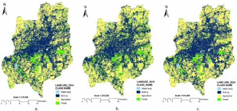
In this study, LULC within Nakhon Ratchasima City was classified into four major categories: agricultural land, built-up and settlement areas, water bodies, and forest areas. The classification was conducted using the SVM algorithm, and its accuracy was validated against high-resolution imagery from Google Earth using 59 independent reference points for each of the three study years: 2014, 2019, and 2024. The results of the accuracy assessment indicate that the classification performed very well, with overall accuracies of 85.66%, 87.97%, and 88.14% for 2014, 2019, and 2024, respectively. The Kappa coefficients exceeded 0.85 in all years, suggesting a strong level of agreement between the classified maps and the reference data. This demonstrates that the LULC classification was reliable and suitable for subsequent analyses.
Spatial analysis of the LULC maps revealed clear patterns of land use transitions over the study period. Agricultural land remained the dominant category, accounting for nearly half of the total area in all years, with a slight increase from 358.88 km² (47.50%) in 2014 to 363.78 km² (48.14%) in 2024. Built-up and settlement areas also exhibited steady growth, expanding from 328.85 km² (43.52%) in 2014 to 335.57 km² (44.41%) in 2024. Conversely, forest areas showed a continuous decline, shrinking from 57.55 km² (7.62%) in 2014 to just 44.28 km² (5.86%) in 2024. Water bodies exhibited a slight increase in extent across the study period. These findings highlight the ongoing transformation of natural and agricultural landscapes into urban and built-up areas, reflecting the district’s role as a rapidly developing economic and social hub in northeastern Thailand. The statistical summary of LULC distribution is presented in Table 3, while spatial patterns of land use change are illustrated in Figure 3.
Table 3. Land use classification within Nakhon Ratchasima City in 2014, 2019 and 2024
|
Land Use Classification |
Water Body |
Built up |
Agriculture |
Forest |
Total |
% OA |
$\widehat{\mathbf{K}}$ |
|
|
2014 |
km2 |
10.32 |
328.85 |
358.88 |
57.55 |
755.60 |
85.66 |
0.89 |
|
% |
1.36 |
43.52 |
47.50 |
7.62 |
100.00 |
|||
|
2019 |
km2 |
11.63 |
331.16 |
362.43 |
50.38 |
755.60 |
87.97 |
0.87 |
|
% |
1.54 |
43.83 |
47.96 |
6.67 |
100.00 |
|||
|
2024 |
km2 |
11.97 |
335.57 |
363.78 |
44.28 |
755.60 |
88.14 |
0.85 |
|
% |
1.59 |
44.41 |
48.14 |
5.86 |
100.00 |
|||
Figure 3. Land use map of Nakhon Ratchasima City in (a) 2014; (b) 2019; (c) 2024
To further examine LULC dynamics, a change detection matrix was generated to compare the classified maps from 2014 and 2019. The results, summarized in Table 4, it was observed that the land use category with the highest stability between 2014 and 2019 was agricultural land, which remained unchanged over an area of 328.57 km², followed by built-up and settlement areas with 298.38 km². This reflects the persistence of agricultural zones and urban land use in areas with continuous development. In contrast, the land categories that contributed most significantly to urban expansion during this period were agricultural land, with 22.48 km² converted to built-up areas, and forest areas, with 8.19 km² converted to urban use. These results highlight a clear trend of agricultural and forest lands being replaced by urban development, emphasizing the growing pressure of urbanization on natural and agricultural landscapes.
When examining the subsequent period (2019–2024), a similar analysis was conducted using a change detection matrix between the two LULC datasets. The results, presented in Table 5, the trend of land use change between 2019 and 2024 remained consistent with the previous period. Agricultural land exhibited the highest level of persistence, with 331.24 km² remaining unchanged, followed by built-up and settlement areas with 301.85 km². Nevertheless, agricultural land was again the most significant contributor to urban expansion, with 23.49 km² converted into built-up areas. Similarly, forest areas experienced a substantial loss of 7.68 km², also being converted into urban land.
Table 4. Change detection matrix 2014-2019
|
Form-to (km²) |
Water Body |
Built up |
Agriculture |
Forest |
|
Water body |
5.26 |
2.16 |
2.29 |
0.61 |
|
Built up |
2.55 |
298.38 |
22.88 |
5.05 |
|
Agriculture |
2.64 |
22.43 |
328.57 |
5.23 |
|
Forest |
1.17 |
8.19 |
8.69 |
39.49 |
Table 5. Change detection matrix 2019-2024
|
Form-to (km²) |
Water Body |
Built up |
Agriculture |
Forest |
|
Water body |
5.85 |
2.54 |
2.57 |
0.66 |
|
Built up |
2.44 |
301.85 |
22.20 |
4.67 |
|
Agriculture |
2.64 |
23.49 |
331.24 |
5.06 |
|
Forest |
1.04 |
7.68 |
7.77 |
33.89 |
These results confirm that the expansion of urban areas in Nakhon Ratchasima City continued to increase steadily during the second study period. The consistent decline of forest areas is particularly concerning, as it may have long-term consequences for ecological integrity and local climate regulation. The findings underscore the dual pressure of urbanization: while it drives economic and social development, it simultaneously intensifies environmental stress through the loss of natural ecosystems and agricultural lands.
3.2 Spatial and temporal trends of land surface temperature (2014–2024)
The spatial and temporal distribution of LST in Nakhon Ratchasima City was analyzed using Landsat 8 (TIR) and Landsat 9 (TIRS-2) imagery for three study periods: 2014, 2019, and 2024. For each period, two seasons were considered, namely winter and summer. To verify the reliability of the satellite-derived LST, validation was conducted against ground-based temperature data obtained from the Nakhon Ratchasima Meteorological Station, operated by the Lower Northeastern Meteorological Center, on the same acquisition dates as the satellite images. The validation results revealed a very high coefficient of determination (R² = 0.9101), along with a Root Mean Square Error (RMSE) of 1.46℃ and a Mean Absolute Error (MAE) of 1.12℃ These low error values confirm that the satellite-derived LST closely represents the actual ground temperature conditions. It is worth noting that slight discrepancies between the two datasets may arise from spatial representativeness differences between the single AWS point measurement and the 30 m Landsat pixel footprint, as air temperature and radiometric surface temperature are not identical physical quantities. Nonetheless, the high correlation and low error metrics indicate that the thermal data from Landsat 8 and Landsat 9 are sufficiently accurate and reliable for subsequent spatial and statistical analyses in this study.
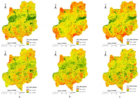
The seasonal trend analysis revealed a pronounced increase in LST during the summer season. The mean LST rose significantly from 29.88℃ in 2014 to 34.14℃ in 2019, before slightly declining to 33.76℃ in 2024. The maximum recorded LST reached 42.86℃ in 2024, which represents a substantial increase compared to the maximum of 36.88℃ in 2014. This pattern reflects the impact of land use transitions, particularly the expansion of built-up areas, which contribute to elevated surface heating. By contrast, the winter season demonstrated more stable conditions, with mean LST values ranging between 25.52℃ and 26.28℃ throughout the study period. The relatively low variability suggests that winter LST in urban areas of Nakhon Ratchasima City remains comparatively stable, with less pronounced effects of land use change compared to the summer season. A summary of the seasonal mean and maximum LST values across the three study years is presented in Table 6.
Figure 4. LST map of Nakhon Ratchasima City by summer and winter season in (a) 2014; (b) 2019; (c) 2024
Table 6. Descriptive statistics of LST for Nakhon Ratchasima City from 2014 to 2024
|
Year / Season |
Mean (℃) |
Maximum (℃) |
Minimum (℃) |
Standard Deviation (℃) |
|
2014_Summer |
29.88 |
36.88 |
20.54 |
1.85 |
|
2014_Winter |
25.52 |
33.45 |
15.84 |
1.25 |
|
2019_Summer |
34.14 |
41.87 |
25.06 |
2.02 |
|
2019_Winter |
26.28 |
35.61 |
16.71 |
1.31 |
|
2024_Summer |
33.76 |
42.86 |
26.65 |
2.02 |
|
2024_Winter |
25.64 |
33.47 |
18.12 |
1.34 |
The spatial patterns of LST across the three study years (2014, 2019, and 2024) are illustrated in Figure 4. The results indicate that areas with consistently high LST values were primarily concentrated in densely populated urban zones and in agricultural lands that had been harvested or left fallow. A major factor contributing to elevated LST in agricultural lands is the absence of vegetation cover following the harvest period, typically between January and April. During this time, bare soil surfaces absorb and retain more solar radiation compared to vegetated areas, resulting in higher surface temperatures. In addition, the common practice of burning crop residues and stubble after harvest further contributes to the increase in surface heating. In contrast, areas with lower LST values were generally located in the central part of the district, corresponding to water bodies, community forests, and agricultural fields with standing crops. The cooling effect of these areas can be attributed to evapotranspiration from vegetation and the reflective properties of tree canopies, both of which help to dissipate heat and reduce surface temperature accumulation.
3.3 ANOVA validation of LST differences among LULC types and seasons
The results of the two-way ANOVA (Table 7) revealed that both season and LULC significantly influenced LST. The effect of season was highly significant (F = 70.646, p < 0.001), indicating that LST during the summer was consistently higher than during the winter. The LULC factor also exhibited a statistically significant effect (F = 4.499, p = 0.006), confirming that built-up and post-harvest agricultural areas recorded higher LST values than forest and water bodies.
Table 7. Two-way ANOVA of LST by LULC and season (2014–2024)
|
Source |
df |
Mean Square |
F |
P-Value |
Partial Eta2 |
|
Season |
1 |
672.204 |
70.646 |
0.000 |
0.525 |
|
LULC Class |
3 |
42.813 |
4.499 |
0.006 |
0.174 |
|
Season * LULC |
3 |
2.757 |
0.290 |
0.833 |
0.013 |
|
Error |
64 |
9.515 |
|
|
|
|
Total |
72 |
|
|
|
|
|
R2 = 0.571; Adj. R2 = 0.524 |
|||||
However, the Season × LULC interaction was not significant (p = 0.833), suggesting that the pattern of seasonal variation was relatively consistent across all land cover types. These findings statistically validate the spatial interpretation of temperature distribution observed in the preceding analysis and confirm that non-vegetated croplands and impervious surfaces act as major heat contributors across seasons.
3.4 Hot spot and cold spot analysis (2014–2024)
The spatial clustering of LST was further examined using the Getis-Ord Gi* statistic, with seasonal differentiation between winter and summer across the three study years (2014, 2019, and 2024). The results indicate that in the summer season, hot spot areas exhibited an increasing trend, rising from 49.63% of the study area in 2014 to 50.76% in 2024. Conversely, cold spot areas decreased slightly, from 45.95% in 2014 to 45.18% in 2024, suggesting a gradual intensification of heat accumulation during summer months. In the winter season, cold spot areas consistently accounted for a greater proportion of the district than hot spots across all study years. For instance, in 2014, cold spots covered 51.50% of the area, compared with 44.50% classified as hot spots. This pattern demonstrates the moderating influence of cooler seasonal conditions on surface temperature distribution. Areas categorized as not statistically significant constituted the smallest proportion in all study periods, averaging less than 5% of the total area. This confirms that the majority of LST variations across the district exhibited statistically significant clustering patterns. A comparison of hot spot and cold spot proportions for each year and season is presented in Table 8.
Table 8. Comparison of hot spot and cold spot proportions for each year and season
|
Year / Season |
Hot Spot (%) |
Cold Spot (%) |
Not Significant (%) |
|
2014_Summer |
49.63 |
45.95 |
4.42 |
|
2014_Winter |
44.50 |
51.50 |
4.00 |
|
2019_ Summer |
50.02 |
45.72 |
4.26 |
|
2019_ Winter |
46.26 |
49.78 |
3.96 |
|
2024_ Summer |
50.76 |
45.18 |
4.06 |
|
2024_ Winter |
47.98 |
48.40 |
3.62 |
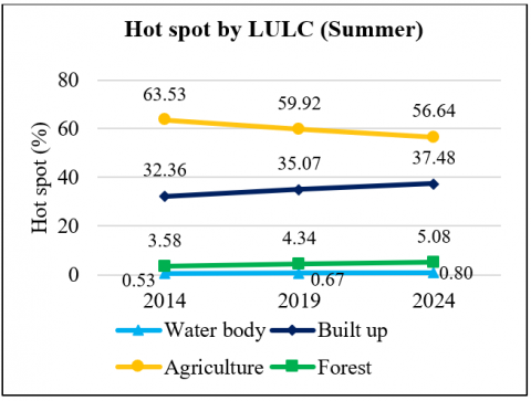
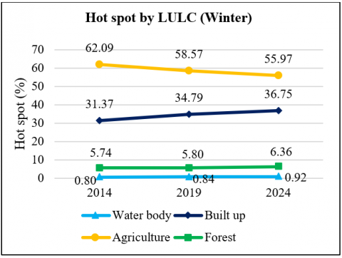
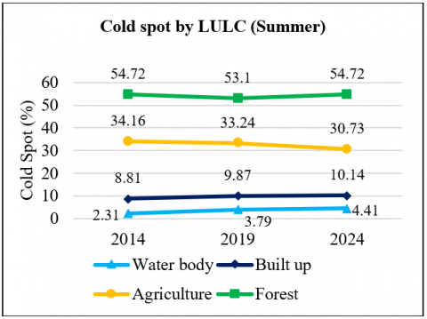
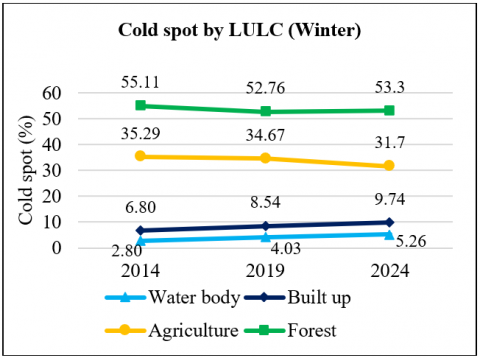
When the results of the Getis-Ord Gi* analysis were integrated with LULC data, seasonal and temporal variations of hot and cold spots were clearly distinguished (Figures 5 and 6).
Figure 5. Comparative hot spot with LULC by summer and winter seasons
Figure 6. Comparative cold spot with LULC by summer and winter seasons
The findings show that agricultural land consistently exhibited a higher tendency to be classified as hot spots compared to cold spots across both seasons. This trend was most pronounced during the summer months throughout all three study years, reflecting the open-surface conditions of post-harvest agricultural fields. These bare soils are directly exposed to solar radiation, thereby accumulating more heat. Moreover, the conversion of agricultural land into built-up areas further contributed to the intensification of hot spots. For built-up and settlement areas, there was a continuous increase in hot spot occurrence across all study periods, particularly during summer. This clearly demonstrates the role of urban expansion and the proliferation of impervious surfaces in amplifying surface heat accumulation. In contrast, forest areas showed a strong and consistent tendency to function as cold spots. They represented the largest proportion of cold spot zones in both summer and winter seasons, highlighting the cooling effects of vegetation cover through shading and evapotranspiration. Similarly, water bodies also exhibited a slight increase in cold spot coverage, especially during the winter season. This pattern can be explained by the thermal properties of water, which moderates temperature fluctuations through heat storage and evaporative cooling, thereby reducing local surface temperatures.
The results of this study demonstrate a clear trend of urban expansion in Nakhon Ratchasima City between 2014 and 2024, particularly during the period 2014–2019. During this interval, urban and built-up areas expanded rapidly at the expense of agricultural and forest lands, reflecting the district’s increasing demand for land to accommodate economic growth and residential development. The spatial pattern of this transformation was most prominent near the city center and along major transportation corridors, underscoring the strong influence of infrastructure development on urban growth dynamics. These findings are consistent with those of Kaewthani and Keeratikasikorn [25], who observed that urban land use in Thailand tends to expand outward from existing urban centers and along major road networks. The results from 2014–2019 align with these broader patterns, suggesting that urban expansion in Nakhon Ratchasima is not an isolated phenomenon but part of a wider trend in urban development in emerging cities. Between 2019 and 2024, the pace of urban expansion continued, with a particularly notable conversion of agricultural land into built-up areas. This indicates an accelerating demand for residential and economic development, potentially associated with road network extensions, new housing projects, and the establishment of emerging economic zones. In contrast, the conversion of urban areas back into agricultural land was minimal, suggesting a steady decline in urban agriculture and reinforcing the trajectory of permanent land use transition. Forest areas also continued to decline, primarily due to conversion into agricultural and urban land, though the rate of loss was slightly lower than in the earlier period. Nonetheless, even modest declines in forested areas are concerning, as they represent a loss of green infrastructure and natural ecosystems that play a critical role in regulating the urban environment. Reduced forest cover contributes to the decline of biodiversity, the loss of ecological services, and the intensification of urban heat through diminished evapotranspiration and shading [6]. These trends highlight the urgent need for more effective land use management policies to protect natural landscapes, particularly forests, in order to mitigate the long-term ecological and climatic impacts of urban expansion.
The analysis of LST dynamics in Nakhon Ratchasima City revealed a pronounced increase in surface temperature during the summer season, particularly between 2014 and 2019, when the mean LST rose by 4.26℃ within a five-year period. This significant increase was concentrated in densely populated urban areas, post-harvest agricultural lands, and open or unused land surfaces, all of which exhibit higher heat accumulation due to the lack of vegetation cover. These findings are consistent with Hu et al. [11], who reported a continuous rise in urban LST between 2001 and 2017, particularly in expanding urban and agricultural areas. Similarly, Teimouri and Karbasi [26] highlighted that open lands and non-vegetated surfaces tend to experience higher surface temperatures compared to cultivated agricultural areas, such as orchards or irrigated farmlands, which benefit from vegetation cover that mitigates heating. The decline of forest cover within the district further exacerbated the rise in LST, as forested areas provide critical cooling effects through shading and evapotranspiration. This result aligns with the findings of Moisa et al. [9], who emphasized that reductions in natural vegetation combined with the expansion of built-up areas significantly increase urban surface heating anomalies. Overall, the results of this study confirm a strong relationship between LULC patterns and LST variability. Areas characterized by urban development and the absence of natural vegetation are particularly vulnerable to elevated surface heating, underscoring the critical role of vegetation cover and sustainable land use planning in mitigating urban heat stress. Similarly, Hasyim et al. [27] demonstrated that land use transformations—particularly the conversion of green spaces into residential areas, commercial zones, and infrastructural developments—have played a critical role in elevating LSTs.
The spatial analysis of LST in Nakhon Ratchasima City, conducted using the Getis-Ord Gi* statistic, revealed a significant relationship between land use and the occurrence of anomalously high-temperature zones (Hot Spots) and low-temperature zones (Cold Spots) across different seasons and study years. Between 2014 and 2024, hot spot areas showed a continuous increase in both summer and winter seasons, particularly in densely populated urban zones and in agricultural lands that were converted or left fallow after harvest. This phenomenon reflects the accelerating process of urban development and the proliferation of infrastructure and built-up structures—such as buildings, roads, and concrete surfaces—that inherently retain and accumulate heat. Consequently, these areas consistently exhibited higher surface temperatures compared to their surroundings. In contrast, cold spot areas declined markedly over the study period, remaining concentrated within forested zones and water bodies. These findings are in line with Guerri et al. [28], who emphasized that urban planning and spatial configuration strongly influence the distribution of hot and cold spots, with key contributing factors including population density, vegetation cover, and topographic conditions. Similarly, Mahata et al. [8] demonstrated that areas with restored water resources or additional tree planting exhibited significant increases in cold spot areas and reductions in hot spots. Taken together, the results underscore the direct influence of urban expansion and LULC changes on the spatial distribution of urban thermal anomalies. They highlight the importance of ecological urban planning, the expansion of green spaces, and the sustainable management of water resources as critical strategies to mitigate the intensification of urban heat and to enhance climate resilience in rapidly developing cities.
Although most studies indicate that urban areas generally exhibit higher LSTs than their rural surroundings—primarily due to dense built-up structures, vehicular emissions, heat-absorbing construction materials, and anthropogenic activities [29]—the findings in Nakhon Ratchasima City reveal an interesting deviation. In some periods, the outer urban fringe, particularly in agricultural fields without vegetative cover and in abandoned open lands, recorded higher LST values than the city center. This phenomenon suggests that the study area has a relatively low potential for pronounced urban heat island (UHI) formation. In fact, in certain seasons, the surrounding rural zones may be warmer than parts of the urban core, especially in open-field agricultural lands left fallow or without vegetation, which absorb more solar radiation and release heat intensively. Moreover, the presence of the city moat, large water bodies, and the relatively high density of urban greenery—including community forests, public parks, shaded residential areas, and tree-lined spaces—contributed to mitigating LST within the city. This aligns with Chuwimonhirun [30], who highlighted the role of urban greenery in lowering surface heat accumulation, and with Getis and Ord [17], who emphasized the cooling effect of surface water bodies through evaporative processes, thereby reducing local heat impacts. Consequently, these results underscore the importance of systematic land use planning both within urban areas and in peri-urban/rural zones. Integrating water bodies, green infrastructure, and vegetation into urban and rural landscapes is essential to regulate LST and sustainably reduce the risks associated with UHI phenomena.
The statistical validation using a two-way ANOVA further reinforces the reliability of the spatial patterns identified in this study. The analysis demonstrated that both season and LULC exert significant effects on surface temperature variation, while their interaction was not statistically significant. This indicates that the seasonal pattern of temperature change remains consistent across different land cover types. The significantly higher mean LST observed in non-vegetated cropland and built-up zones quantitatively supports the “reverse-UHI” phenomenon identified in spatial analysis. In peri-urban areas, bare agricultural fields—particularly after harvest during the pre-monsoon dry season—act as transient heat sources, surpassing even the urban core in surface temperature. These findings provide robust statistical confirmation that land management and vegetation cover strongly regulate surface thermal dynamics in tropical monsoon environments such as Nakhon Ratchasima City.
The reliability of the satellite-derived LST used in this study was confirmed through validation with ground-based observations from the Nakhon Ratchasima Meteorological Station. The comparison yielded a very strong correlation (R² = 0.9101) and low error values (RMSE = 1.46℃, MAE = 1.12℃), indicating that the retrieved LST accurately represents real surface thermal conditions. These results are consistent with previous findings [21] demonstrating that Landsat thermal data can provide reliable temperature estimates for mesoscale urban analyses when appropriately calibrated. Nonetheless, minor discrepancies between satellite and ground temperatures are expected due to differences in measurement scales and physical properties: satellite sensors measure radiometric surface temperature, whereas meteorological stations record air temperature at approximately 2 m above ground. Furthermore, the 30 m Landsat pixel integrates spatial heterogeneity—such as vegetation, built surfaces, and bare soil—within its footprint, while the meteorological station represents a single point. Despite this spatial mismatch, the low error metrics observed in this study confirm that the LST retrievals are robust and sufficiently representative for subsequent spatial-statistical analyses. Future validation efforts could benefit from multiple AWS sites and the use of spatial averaging (e.g., 3 × 3 window) to further reduce point–pixel discrepancies.
This study analyzed land use/land cover (LULC) changes, spatial distribution trends of LST, and the occurrence of statistically significant hot and cold spots in Nakhon Ratchasima City between 2014 and 2024. Landsat satellite imagery combined with spatial analysis using the Getis-Ord Gi* statistic was employed. The findings can be summarized as follows: Land Use/Land Cover Change. Built-up areas have continuously expanded, particularly in zones adjacent to the city center and along major road networks. Most of these expansions replaced agricultural and forest lands, reflecting the pressure of rapid urbanization and the increasing demand for land for development and residential purposes. Surface Temperature Trends. LST values in summer were higher than in winter and showed a distinct increasing trend, especially between 2014 and 2019, when the average temperature rose by more than 4℃. High-temperature zones were concentrated in built-up areas, bare agricultural lands, and open spaces, whereas forested areas and water bodies played a critical role in regulating and lowering surface temperatures. Hot and Cold Spot Distribution. Hot spots have increased steadily in both summer and winter, clustering in urban and abandoned agricultural lands. Conversely, cold spots have gradually declined, mainly concentrated in forested areas and water bodies. This indicates a statistically significant spatial relationship between land use patterns and surface temperature variation. Urban–Rural Temperature Patterns. Interestingly, in certain periods, non-vegetated agricultural lands and abandoned open fields in the suburban fringe recorded higher LST values than the city center. This suggests that the intensity of the urban heat island (UHI) phenomenon in this study area is relatively low. A key factor is the city’s landscape structure, which still retains protective elements such as the historical moat, large urban ponds, and dispersed green areas—including public parks, community forests, and tree-covered residential zones—that contribute to surface temperature reduction.
Despite these contributions, several areas remain open for further research. Future studies should integrate additional climatic and environmental parameters, such as wind speed, humidity, soil moisture, and air pollution (e.g., PM2.5), to capture a more comprehensive picture of local thermal dynamics. Expanding temporal coverage to include additional seasons and higher-frequency observations would enhance the understanding of year-round thermal variability. The use of high-resolution and multi-source data, including Sentinel-2, PlanetScope, or UAV-based thermal imaging, would further improve fine-scale detection of micro-urban heat island effects. Predictive modeling approaches, such as Cellular Automata–Markov simulations or machine learning–based urban growth models, could provide valuable forecasts of future LULC and LST scenarios. Additionally, incorporating socioeconomic and health dimensions would strengthen the relevance of research findings, particularly regarding the impacts of thermal anomalies on energy use and public health risks.
This research provides new empirical evidence linking multi-temporal LULC transitions with spatial thermal anomalies in a rapidly developing provincial city—an aspect rarely investigated in Thailand’s urban climate literature. By integrating SVM classification, satellite-derived LST retrieval, and Getis-Ord Gi* hotspot analysis within a single framework, the study demonstrates an effective methodological approach for identifying statistically significant heat and cooling zones. Notably, the detection of potential “reverse-UHI” conditions in post-harvest croplands represents a unique contribution, suggesting that certain non-urban landscapes can temporarily generate higher surface temperatures than dense urban cores. These insights expand the theoretical understanding of urban–rural thermal interactions in tropical environments and fill a critical research gap in medium-sized Thai cities.
Statistical evidence from the two-way ANOVA analysis confirmed the significant effects of both land use/land cover and seasonal variation on LST. The results quantitatively substantiate the “reverse-UHI” phenomenon observed in peri-urban cropland areas, emphasizing that open and non-vegetated lands can act as temporary heat sources during the dry season. This evidence reinforces the importance of integrating land use planning, green-space preservation, and seasonal climate considerations into sustainable urban development strategies.
Beyond its empirical results, this study contributes to refining urban-climate theory in tropical environments. The observed “reverse-UHI” tendency—where post-harvest croplands and bare peri-urban fields occasionally exhibit higher surface temperatures than urban cores—suggests that non-urban landscapes can act as transient heat sources during dry or pre-monsoon periods. This finding challenges the conventional assumption that urban areas are always the dominant heat emitters and highlights the temporal dimension of heat dynamics in mixed urban–agricultural settings. It emphasizes that urban heat phenomena in tropical cities are not solely determined by built-up intensity but also by seasonal vegetation cycles, soil exposure, and land management practices. Such insights extend existing UHI frameworks toward more nuanced interpretations of land–atmosphere interactions across urban–rural gradients.
The findings of this study align closely with the objectives of the United Nations Sustainable Development Goal 11 (SDG 11), which promotes inclusive, safe, resilient, and sustainable cities. Specifically, the emphasis on preserving urban green infrastructure and restoring water bodies directly supports SDG 11.3 on sustainable urbanization and SDG 11.7 on ensuring universal access to green public spaces. At the provincial level, the results provide scientific evidence that can inform the Nakhon Ratchasima Provincial Spatial Plan [18], particularly concerning the designation of urban growth zones, ecological buffer areas, and green corridors. Integrating RS–based thermal analysis into local planning frameworks would enhance the province’s capacity to mitigate heat stress, promote environmental resilience, and guide land-use decisions toward long-term sustainability.
The findings carry important implications for sustainable urban development and climate adaptation planning. Urban ecological planning should prioritize the preservation and expansion of green infrastructure, such as public parks, community forests, and tree-lined neighborhoods, which play a critical role in mitigating urban heat. The protection and restoration of water bodies should also be emphasized, as they contribute significantly to evaporative cooling and resilience against extreme heat events. Furthermore, stronger land use regulations and zoning policies are necessary to balance urban growth with environmental sustainability, limiting the uncontrolled conversion of agricultural and forest land into built-up areas. Finally, sustainable urban design interventions—including the use of green roofs, permeable pavements, and reflective construction materials—offer practical solutions to reduce surface heat accumulation in rapidly growing cities.
The author gratefully acknowledges the Lower Northeastern Meteorological Center for supplying ground-based temperature observations from meteorological stations in Nakhon Ratchasima Province, which were essential for validating the satellite-derived results and ensuring the successful completion of this study.
[1] Khalid, W., Kausar Shamim, S., Ahmad, A. (2024). Exploring urban land surface temperature with geospatial and regression modelling techniques in Uttarakhand using SVM, OLS and GWR models. Evolving Earth, 2: 100038. https://doi.org/10.1016/j.eve.2024.100038
[2] Alexander, C. (2020). Normalised difference spectral indices and urban land cover as indicators of land surface temperature (LST). International Journal of Applied Earth Observation and Geoinformation, 86: 102013. https://doi.org/10.1016/j.jag.2019.102013
[3] Avashia, V., Garg, A., Dholakia, H. (2021). Understanding temperature related health risk in context of urban land use changes. Landscape and Urban Planning, 212: 104107. https://doi.org/10.1016/j.landurbplan.2021.104107
[4] Fu, P., Weng, Q. (2016). A time series analysis of urbanization induced land use and land cover change and its impact on land surface temperature with Landsat imagery. Remote Sensing of Environment, 175: 205-214. https://doi.org/10.1016/j.rse.2015.12.040
[5] Khan, N., Shahid, S., Sharafati, A., Yaseen, Z.M., Ismail, T., Ahmed, K., Nawaz, N. (2021). Determination of cotton and wheat yield using the standard precipitation evaporation index in Pakistan. Arabian Journal of Geosciences, 14(19): 2035. https://doi.org/10.1007/s12517-021-08432-1
[6] Guha, S., Govil, H., Gill, N., Dey, A. (2020). Analytical study on the relationship between land surface temperature and land use/land cover indices. Annals of GIS, 26(2): 201-216. https://doi.org/10.1080/19475683.2020.1754291
[7] Gupta, N., Mathew, A., Khandelwal, S. (2019). Analysis of cooling effect of water bodies on land surface temperature in nearby region: A case study of Ahmedabad and Chandigarh cities in India. The Egyptian Journal of Remote Sensing and Space Science, 22(1): 81-93. https://doi.org/10.1016/j.ejrs.2018.03.007
[8] Mahata, B., Sankar Sahu, S., Sardar, A., Laxmikanta, R., Maity, M. (2024). Spatiotemporal dynamics of land use/land cover (LULC) changes and its impact on land surface temperature: A case study in New Town Kolkata, eastern India. Regional Sustainability, 5(2): 100138. https://doi.org/10.1016/j.regsus.2024.100138
[9] Moisa, M.B., Dejene, I.N., Gemeda, D.O. (2022). Integration of geospatial technologies with multiple regression model for urban land use land cover change analysis and its impact on land surface temperature in Jimma City, southwestern Ethiopia. Applied Geomatics, 14(4): 653-667. https://doi.org/10.1007/s12518-022-00463-x
[10] Qu, S., Wang, L., Lin, A., Yu, D., Yuan, M., Li, C. (2020). Distinguishing the impacts of climate change and anthropogenic factors on vegetation dynamics in the Yangtze River Basin, China. Ecological Indicators, 108: 105724. https://doi.org/10.1016/j.ecolind.2019.105724
[11] Hu, M., Wang, Y., Xia, B., Huang, G. (2020). Surface temperature variations and their relationships with land cover in the Pearl River Delta. Environmental Science and Pollution Research, 27(30): 37614-37625. https://doi.org/10.1007/s11356-020-09768-z
[12] Pal, S., Ziaul, S. (2017). Detection of land use and land cover change and land surface temperature in English Bazar urban centre. The Egyptian Journal of Remote Sensing and Space Sciences, 20(1): 125-145. https://doi.org/10.1016/j.ejrs.2016.11.003
[13] Yan, D., Yu, H., Xiang, Q., Xu, X. (2023). Spatiotemporal patterns of land surface temperature and their response to land cover change: A case study in Sichuan Basin. The Egyptian Journal of Remote Sensing and Space Sciences, 26(4): 1080-1089. https://doi.org/10.1016/j.ejrs.2023.12.002
[14] Ahmad, M., Saqib, M., Ahmad, S.N., Jamal, S., Mir, A.Y. (2025). Normalized difference spectral indices and urban land cover as indicators of urban heat island effect: A case study of Patna Municipal Corporation. Geology, Ecology, and Landscapes, 1-21. https://doi.org/10.1080/24749508.2025.2451479
[15] Creţu, Ş.C., Sfîcă, L., Ichim, P., Amihăesei, V.A., Breabăn, I.G., Roşu, L. (2025). Warm season land surface temperature and its relationship with local climate zones in post-socialist cities. Theoretical and Applied Climatology, 156(4): 191. https://doi.org/10.1007/s00704-025-05409-y
[16] Addas, A., Goldblatt, R., Rubinyi, S. (2020). Utilizing remotely sensed observations to estimate the urban heat island effect at a local scale: Case study of a university campus. Land, 9(6): 191. https://doi.org/10.3390/land9060191
[17] Getis, A., Ord, J.K. (1992). The analysis of spatial association by use of distance statistics. Geographical Analysis, 24(3): 189-206. https://doi.org/10.1111/j.1538-4632.1992.tb00261.x
[18] Department of Public Works and Town and Country Planning. (2016). Nakhon Ratchasima provincial comprehensive plan project. The 2nd Public Hearing on Provincial Comprehensive Planning, Nakhon Ratchasima, Thailand. https://www.nettathai.org/upload/03-1%20-.pdf.
[19] Nakhon Ratchasima Provincial Statistical Office. (2024). Demographic, population and housing statistics. https://nkrat.nso.go.th/images/stitic/5/stat_1.pdf.
[20] Landis, J.R., Koch, G.G. (1977). The measurement of observer agreement for categorical data. Biometrics, 33(1): 159. https://doi.org/10.2307/2529310
[21] Weng, Q., Lu, D., Schubring, J. (2004). Estimation of land surface temperature-vegetation abundance relationship for urban heat island studies. Remote Sensing of Environment, 89(4): 467-483. https://doi.org/10.1016/j.rse.2003.11.005
[22] Jesus, J.B.D., Santana, I.D.M. (2017). Estimation of land surface temperature in caatinga area using Landsat 8 data. Journal of Hyperspectral Remote Sensing, 7(3): 150-157. https://doi.org/10.29150/jhrs.v7.3.p150-157
[23] Jackson, R.D., Huete, A.R. (1991). Interpreting vegetation indices. Preventive Veterinary Medicine, 11(3-4): 185-200. https://doi.org/10.1016/S0167-5877(05)80004-2
[24] Tran, D.X., Pla, F., Latorre-Carmona, P., Myint, S.W., Caetano, M., Kieu, H.V. (2017). Characterizing the relationship between land use land cover change and land surface temperature. ISPRS Journal of Photogrammetry and Remote Sensing, 124: 119-132. https://doi.org/10.1016/j.isprsjprs.2017.01.001
[25] Kaewthani, S., Keeratikasikorn, C. (2019). Improving SLEUTH urban growth model using logistic regression and land density function. International Journal of Geoinformatics, 15(3): 65-79. https://journals.sfu.ca/ijg/index.php/journal/article/view/1857.
[26] Teimouri, R., Karbasi, P. (2024). Analyzing the contribution of urban land uses to the formation of urban heat islands in Urmia City. Urban Science, 8(4): 208. https://doi.org/10.3390/urbansci8040208
[27] Hasyim, A.W., Sukojo, B.M., Fatahillah, E.R., Anggraini, I.A., Isdianto, A. (2025). Assessing the impact of population density and land use on land surface temperature for sustainable urban planning in Malang City, Indonesia. International Journal of Sustainable Development and Planning, 20(5): 1679-2197. https://doi.org/10.18280/ijsdp.200533
[28] Guerri, G., Crisci, A., Messeri, A., Congedo, L., Munafò, M., Morabito, M. (2021). Thermal summer diurnal hot-spot analysis: The role of local urban features layers. Remote Sensing, 13(3): 538. https://doi.org/10.3390/rs13030538
[29] Kleerekoper, L., van Esch, M., Salcedo, T.B. (2012). How to make a city climate-proof, addressing the urban heat island effect. Resources, Conservation and Recycling, 64: 30-38. https://doi.org/10.1016/j.resconrec.2011.06.004
[30] Chuwimonhirun, T. (2013). The influence of water surface on temperature: A case of Sathorn Commercial Zone, Bangkok. Asian Creative Architecture, Art and Design, 15(2): 133-148. https://www.thailis.or.th/tdc/browse.php?option=show&browse_type=title&titleid=317215.