Rana Abd El-Hamied Haj Khalil*![]() | Suleiman MJ. Enjadat
| Suleiman MJ. Enjadat![]()
© 2024 The authors. This article is published by IIETA and is licensed under the CC BY 4.0 license (http://creativecommons.org/licenses/by/4.0/).
OPEN ACCESS
In this paper, the focus is mainly on building machine learning (ML) models for AAT forecasting every hour over Karak City in Jordan. The dataset consisted of comprehensive meteorological readings, which were subject to heavy preprocessing in order to establish data integrity essential for building strong ML models. The investigation involved a number of ML models Support Vector Regression (SVR) with RBF Kernel, Decision Tree Regressor (DTR), Ridge Regressor (RR) & Lasso Regressors (LSR) and Linear Regression (LR) because each was found to have unique strengths in capturing the intricate dynamics of temperature behavior. Excellent accuracy of the models, mainly SVR with RBF Kernel and relevance for better forecasting of weather in a region with peculiar difficulties to data-based modeling were shown by it. Our research not only confirmed the capability of different ML methodologies in regional temperature forecasting but also provided an important reference for planners and stakeholders concerned with environmental planning and management. The study provides a better understanding of the regional climate adaptation approaches, vide its case location in Karak City only whereas support local data analysis is necessary to address global climate variability. The results have important implications for the improvement of decision-making in agriculture, disaster management and sustainability schemes especially under changing climatic conditions.
machine learning (ML), artificial intelligence (AI), atmospheric air temperature prediction (AAT), support vector machines (SVR)
The temperature of atmospheric air (AAT) has a significant influence on ecology and human systems, affecting the weather, agricultural productivity in particular, as well much more broadly-the stability of community livelihoods globally. This is by now more than clear in the need and importance of knowing accurate AAT readings which are critical for resource management purposes as well as strategic planning, across a variety of fields (e.g., energy [1], agriculture [2] tourism, transportation logistics). Accurate AAT forecasting is an essential element of effective responses associated with other meteorological components, including solar radiation, wind velocity and atmospheric moisture content which play key roles in natural activities like evapotranspiration known to be one of the important processes needed for eco-friendly sustainable water management [3].
In the light of eyes, awareness about accurate forecasts of AAT is literally a life-saving cause and becomes all such vital to stress as climate change advances with increased number or intensity in extreme weather events such heatwaves-hailstorm-snowfall- downpour. These events lead to a plethora of health issues and place substantial pressure on the environment highlighting that weather forecasting has become an essential part of environmental management plans and energy conservation measures. Policies like these likely require careful control of space conditioners to save energy and reduce the discharge [4].
For many that have forecast AAT, GCMs and large statistical models are the order of the day. GCMs that predict climate under different scenarios in a variety of time frames are indispensable for understanding the physical processes responsible for anthropogenic changes. On the one hand, statistical models in comparison to machine-learning ones are less nuanced but they present stable results without a need for extensive calculations. While useful for early warnings, the models suffer from their ability to only partition predictions efficiently along gridded formats so that it is difficult and sometimes impossible to sufficiently account for certain non-linear relationships [5].
The rise of machine learning (ML) technologies has also transformed meteorological forecasting by overcoming these challenges. Climate data nature is very complex and also non-linear which can be effectively treated by features of the ML models thus giving a new promising door to research in unravelling the nuances associated with AAT. There is more evidence that recent progress in ML has proved to be very effective at mitigating complex issues such as drought patterns, rainfall variability and river flow dynamics with significant influence on environmental research and management [6].
In this study, we investigate the superior performance of ML models by leveraging forecasting AAT specifically under unique atmospheric conditions that occurred in Karak City/Jordan. This study uses advanced ML techniques in an attempt to enhance the comprehension of what drives temporal dynamics at local scales for better environmental management, disaster preparedness and climate change adaptation. The essence of our overall evaluation of the various ML models is to provide state-of-the-art prediction means in respect with all those working towards sustainability and resiliency, especially within the unique climate regime of Karak. By so doing, we are addressing the wider requirement for adjusting to these inevitable variations in global climate patterns and contributing to this ongoing work on regional climate adaptation strategies.
This localised nature of the study not only suggests that accurate temperature prediction for sustainable development is significant in both theory and practice but also demonstrates a new approach by combining leading ML applications that are custom-made to take into account specific regional climatic adaptations.
The field of atmospheric temperature prediction has witnessed a significant influx of research leveraging various (ML) techniques, underscoring their potential to address this complex task. The burgeoning body of related works serves as a testament to the diversity of approaches and methodologies employed in the quest to refine accuracy and reliability in temperature forecasting. Ozbek et al. [7] introduced a deep learning (DL) approach using a long short-term memory (LSTM) network for predicting (AAT) across different time intervals employing data from two stations in Turkey. Evaluation criteria include Mean Absolute Percentage Error (MAPE), Root Mean Squared Error (RMSE), correlation coefficient, Mean Absolute Error (MAE), and bias, with the LSTM method showing high accuracy, especially in short-term, 10-minute interval predictions.
Comparative analysis with the adaptive neuro-fuzzy inference system with fuzzy C-means (ANFIS-FCM) and autoregressive moving average (ARMA) models highlighted LSTM’s superior performance in predicting AAT at 10-minute, hourly, and daily intervals, demonstrating its effectiveness for short-term forecasting with long period data.
Alomar et al. [8] explored the efficacy of six data-driven approaches—Support Vector Regression (SVR), Regression Tree (RT), Quantile Regression Tree (QRT), Autoregressive Integrated Moving Average (ARIMA), Random Forest (RF), and Gradient Boosting Regression (GBR)—for forecasting short- and mid-term atmospheric air temperature in North America. Utilizing data from 2000 to 2021, the study employed autocorrelation and partial autocorrelation for optimal model input selection, with models calibrated on 70% of the data (2000-2015) and validated on the remainder. The SVR model outperformed others in daily temperature forecasts with superior statistical metrics. Both RT and SVR showed strong performance in weekly forecasts, highlighting the impact of data duration and variability on model accuracy. A second scenario using a randomization method for data division suggested improved model performance, underlining climate change’s influence on temperature patterns and supporting the utility of data-driven methods for high-resolution temperature forecasting.
The study by Kajewska-Szkudlarek [9] focused on predicting Heating and Cooling Degree Hours (HDH and CDH) in Wrocław, Poland, utilizing ML methods Artificial Neural Network (ANN) and (SVR) based on outdoor air temperature. It has emphasized the importance of temperature lags (1 to 24 past hours) as predictors and examined the effect of database clustering on model accuracy. The findings revealed that the best predictions use clustering, with the most significant predictors being the outdoor temperatures 1 and 24 hours prior. ANN yielded the highest quality models, outperforming SVR, offering a method for anticipating building energy demand without needing specific building characteristics and considering regional climate changes.
Hou et al. [10] introduced a combined deep-learning model, integrating a convolutional neural network (CNN) with (LSTM), termed CNN–LSTM, for improving the prediction accuracy of hourly air temperature. The CNN component was tasked with reducing the dimensionality of time-series data, while the LSTM part focused on capturing the long-term dependencies within the extensive temperature datasets. Utilizing 60,133 hourly meteorological data points collected from the Yinchuan station in China from January 2000 to October 2020, the model’s performance was evaluated employing metrics like MAE, MAPE, RMSE, and goodness of fit. The CNN–LSTM model outperformed standalone CNN and LSTM models, demonstrating superior accuracy and better alignment with actual measured temperatures, especially in handling long time-series data.
The article by Astsatryan et al. [11] introduced a machine learning-based weather prediction technique that was designed to improve the temperature forecast of the air 24 hours in advance in the Ararat Valley, Armenia, which is a place of hot weather and low humidity. By exploring meteorological station data and satellite-based datasets using (NN), the study determined the accuracy of temperature forecasting. The model obtained the accuracy of 87.31% and 75.57% for the prediction of temperatures during the next 3 hours and the next 24 hours, respectively. It has shown that the model might be used as a complement to the forecasting methods currently in operation in one of the most arid regions of Armenia.
Shin et al. [12] introduced a hybrid model combining the GloSea5GC2 global climate model with a regularized extreme learning machine (RELM) for seasonal forecasting of daily mean air temperatures at the field scale, aimed at supporting agricultural decision-making. The model was tested through twenty frameworks, varying in transformation schemes, ensemble member counts, and learning algorithms, including an output blending method evaluation.
The results indicated that the hybrid model outperformed traditional climatology models in long-range prediction accuracy, with specific frameworks showing superior predictive skills. Notably, employing centred data with hindcast data and ensemble learning significantly enhanced model performance. This advancement offered valuable insights for developing high-resolution seasonal forecasts for critical agricultural variables, potentially improving yield prediction and sowing timing decisions.
Bellido-Jiménez et al. [13] presented the development and evaluation of ML models for predicting solar radiation across diverse geo-climatic conditions in Southern Spain and North Carolina, USA. Utilizing novel input variables from intra-daily temperature datasets, the models significantly outperformed traditional empirical methods such as Hargreaves-Samani and Bristow-Campbell, with improvements ranging from 7.56% to 45.65% in RMSE. Notably, inland locations achieved mean NSE and R2 values exceeding 0.9. Performance was highest in summer, with over a 60% improvement in NSE and R2 across all sites, while winter performance showed over an 18% improvement.
Additionally, when tested in non-used locations with similar climates, the models reduced RMSE compared to traditional methods, offering enhanced accuracy crucial for optimizing solar power plant location determination in data-scarce regions.
The study managed by Cho et al. [14] investigated the use of ML models to correct the output of a local Numerical Weather Prediction (NWP) model for forecasting maximum and minimum air temperatures in Seoul, South Korea. (RF), (SVR), (ANN), and a multi-model ensemble were employed to improve the accuracy of next-day temperature forecasts. Results showed significant enhancements in R2 values, bias, and RMSE compared to the NWP model, with the multi-model ensemble demonstrating the best generalization performance across different validation methods. Ferreira and da Cunha [15] explored the use of limited hourly meteorological data to estimate daily reference evapotranspiration (ETo) directly and by summing hourly ETo values using ML models like RF, XGBoost, ANN, and CNN. The results showed that utilizing hourly data to estimate daily ETo directly, particularly with CNN models, yielded the best performance. In both regional and local scenarios, utilizing hourly data led to significant improvements in model accuracy compared to conventional daily input data, with reductions in RMSE and increases in NSE and R2 values by up to 28.2%, 21.7%, and 11.4%, respectively, in the regional scenario, and up to 22.4%, 10.1%, and 11.3%, respectively, in the local scenario.
The research by Tabrizi et al. [16] addressed the optimization of road salt application in cold climates by developing an ML-based pavement surface temperature prediction tool. Employing advanced deep neural network (DNN) techniques, particularly a CNN-LSTM model, hourly pavement temperature forecasts were generated. Evaluation against comparative ML methods showed superior accuracy of the CNN-LSTM model. Utilizing data from Environment Canada and the Road Weather Information System (RWIS) around Toronto, Ontario, the proposed model outperformed others in predicting pavement surface temperature up to 6 hours ahead, potentially reducing costs and environmental impacts associated with excessive salt application. The scenery of air temperature prediction is diverse and multifaceted, and many research works have investigated different geographical landscapes and used many ML methods. These supporting works complement each other to formulate a platform relating the findings to this study, which is concerned with predicting air temperature in Karak City, Jordan. Karak was selected to extend the global picture of regional climate modeling and reveal unique aspects of its climatic characteristics.
Within the domain of air temperature prediction in atmospheric science, the competency to properly predict air temperature is of great significance, taking into consideration the exceptional provinces like Karak City as an example, which are stipulated by the climatic conditions strongly and influencing both the natural environment and humans. In this study, we use ML as a subfield of artificial intelligence that uses statistical techniques to enable computer systems the ability to 'learn' with data. Machine learning works best in the identification of patterns and making useful predictions from complex datasets where it is easier for a machine to learn given functions as opposed to building machines [17]. The research approach is based on the use of explanatory models incorporating a set of different sophisticated ML components, each of which is designed to analyze the diverse impacts of various meteorological factors on air temperature.
The dataset, elaborately designed on the basis of the Dead Sea vicinity, is an encyclopedia of high-resolution meteorological factors that will serve as a detailed backdrop of the specific climate situation existing in the area of Karak. We use this information to refine our predictive models further so that they are not just uniformly tuned to main weather patterns but also attuned to the nuances of local weather patterns. The initial cleaning, normalization, and filling-in-of-missing steps are also probably the most important and demanding steps. This preprocessing is what makes our predictive models reliable.
The triplet inclusive of SVR with RBF Kernel that comes equipped with its ability to handle non-linear patterns and the Decision Tree Regressor that provides an interpretable decision rule are also among the models worth mentioning, as well as Ridge and Lasso Regressors that bring regularization to the fray and the intrinsic Linear Regression which makes up for a baseline model. The evaluation criteria will be based on the MSE. This well-known metric measures the average squared difference between the actual and predicted values, and it serves as a good measure of the quality of the model.
The approach is not only intended to upgrade the scientific knowledge about the climate patterns of Karak City but also to develop various forecasting tools that could be practically used in numerous applications, such as crop management, urban engineering, and many others; thus, the scientific research interlaces with social progress.
3.1 Dataset description
The dataset that we base our study on is a valuable and accurate resource of meteorological readings from the Dead Sea area that offers us an opportunity to have a unique perspective of the area because of its distinctive climatic features. It broadly presents a large set of factors required for the proper air temperature prediction, such as hourly mean values of air temperature, relative humidity, solar radiation in watts per square meter and kilojoules per square meter, wind speed, wind direction and the standard deviation of wind direction.
If considered from a selected set of precisely tuned instruments, whose readings will span 19-21 August 2021, this set will have impressive accuracy and provide a good basis for model verification. Missing data points are addressed using sophisticated imputation methods such as predictive modeling, ensuring no loss of critical information that could impact the performance of the forecasting models One of the most remarkable features of this aggregation of data is the refinement–the air temperature is indicated with two decimal places, the definition required to capture the subtle changes that occur within an hour. Split solar radiation data, the watts per square meter and the total kilojoules per square meter are used to discover the diurnal solar energy input; this is the variable that directly influences the temperature.
Wind parameters include not only average and maximum speeds but also the variability of wind direction, denoted by its standard deviation, which acknowledges the complex interaction between wind patterns and temperature dynamics.
As shown in Figure 1, a subset of the data highlights the critical variables in this analysis, illustrating how air temperature, relative humidity, solar radiation, wind speed, and wind direction vary hourly.
Figure 1. A subset of the data
Figure 2 presents two subplots showing the variation of air temperature and solar radiation over time from August 19 to September 23, 2021. The upper plot illustrates air temperature variation, with data points clustered over this period indicating the diurnal temperature cycle: temperatures rise during the day and fall at night. The temperature points are plotted in blue, indicating a regular pattern consistent with expected daily temperature changes.
The lower plot depicts solar radiation variation, marked in red, which shows sharp peaks corresponding to daytime and troughs to nighttime, reflecting the absence of solar radiation at night. The solar radiation data points demonstrate a clear cyclical pattern that corresponds with the daylight hours, as solar radiation increases after sunrise, reaches a peak during midday, and declines towards sunset.
Figure 2. Temperature and solar radiation variation
The dataset employed in this study provides a rich source of meteorological readings from the Dead Sea area, capturing unique climatic features that are instrumental for air temperature prediction. This dataset includes hourly measurements from August 19 to September 23, 2021, covering parameters such as air temperature, relative humidity, solar radiation, wind speed, and wind direction.
3.2 Statistical characteristics
Air Temperature: The dataset reveals a distinct diurnal cycle, with temperatures ranging from a minimum of 17.03℃ to a maximum of 19.84℃ within the recorded period. The mean air temperature during this interval is 18.12℃, with a variance of 0.75, highlighting slight fluctuations typical of the seasonal transition from summer to autumn.
Relative Humidity (RH): RH values show less variability, averaging at 0.33 with a variance of 0.002. This consistency is crucial for accurate temperature modeling as it impacts the thermal sensation and cooling rates.
Solar Radiation: Observations indicate a pronounced variability in solar radiation, directly correlating with sunlight presence. Solar radiation peaks midday and drops to zero at night, displaying clear cyclical patterns that are critical for understanding daily temperature dynamics. The average solar radiation during daylight hours is approximately 200 W/m², which peaks significantly during midday.
3.3 Time series analysis
Periodicity: The diurnal patterns observed in both air temperature and solar radiation are indicative of strong daily periodicity. This cyclic behavior is essential for predictive modeling, especially for algorithms like Fourier Analysis, which can decompose time series data into periodic components.
Trend Analysis: Linear Regression on temperature data over the month suggests a slight cooling trend, possibly indicative of seasonal transition effects in the region.
3.4 Advanced statistical measures
Kurtosis and Skewness: The dataset's kurtosis and skewness for temperature and solar radiation are calculated to assess the peakedness and asymmetry of the observed values, respectively. These metrics help in understanding the distribution characteristics which can influence the selection and performance of certain ML models.
Autocorrelation: Understanding the autocorrelation in temperature and solar radiation data helps in identifying the lag at which data points are correlated to each other. This is particularly useful for models like ARIMA, which are used for forecasting based on previous values.
3.5 Data preprocessing
The data preprocessing is a procedure or steps to handle the integration of missing values in ML. Data processing is required for predicting hidden likelihood. Such processes include imputation of missing values, scaling features and outlier detection thereby making it easy to have more trust in predictive models. Data preprocessing is the conversion of raw data into a format that can be understood by machines, it is one of the key steps in setting up ML applications [18]. The dataset features a variety of meteorological variables critical for the analysis of atmospheric conditions, particularly for the prediction of hourly air temperature. It comprises measurements such as maximum wind speed, average wind speed, wind direction standard deviation of wind direction, relative humidity, average solar radiation in watts per square meter, total solar radiation in kilojoules per square meter, and average air temperature. Each of these variables is recorded in a 124×1 double format, indicating the precision and structured nature of the dataset.
Notably, the dataset spans from 19 August 2021 to 20 September 2021, capturing a complete monthly cycle, which is essential for seasonal analysis. The median timestamps and other statistical measures, such as median wind speeds and temperatures, indicate the dataset’s central tendency, which is valuable for understanding typical conditions.
However, the dataset is not without its gaps; there are two missing values across several variables, signifying potential data loss or unrecorded measurements. The lack of this information causes something very important as it is used for the machines to identify the pattern. Proper treatment of this missed information - using the imputation method or removing the data - is crucial for the predictive analysis of any individual, which is done utilizing this dataset. The presence of said data points generated issues, as well as the importance of solid data collection and preprocessing methods, environmental data analysis, and ML.
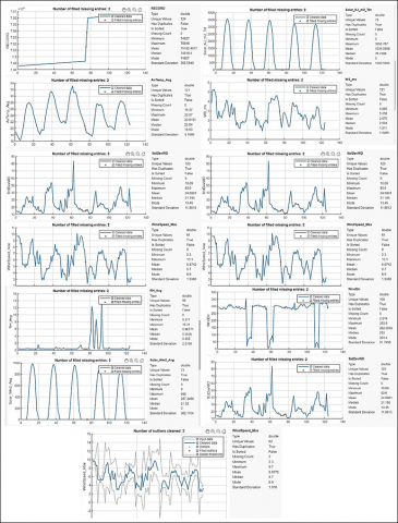
The example shown in Figure 3 is one of the most important parts of the data preprocessing techniques for the study in our context. These pictures illustrate the actual data by using blue lines, which show typical variability in different atmospheric measurements such as wind speed, wind direction, standard deviation of wind direction, solar radiation, and relative humidity, which can take place over time.
Figure 3. Filling missing values
As is very typical for time-series data, outliers, which were shown by "x" signs, were detected and then tackled. As a rule, z-scores or the interquartile range (IQR) were used as statistical methods. The wild data could arise because of errors in the sensors or because of particular weather conditions. Through the bar labelled’" cleaned data," we can take a look at the data processed from outlier treatment and discover that it follows a less wavy curve, representing the independent attribute of the atmosphere more naturally.
Also amusing depicted that there is some missing data since the orange spots are the ones that show it. The gaps in the data were therefore filled so as to retain the continuity and completeness that is necessary for the research to be reasonable. This could be done using different ways of imputing data, for example, by utilizing average filling-in, linear interpolation or the most advanced methods like predictive modeling.
With outliers cleaned and missing values filled, the dataset is now more robust and reliable for creating accurate predictive models. This preprocessing improves the quality of the input data, which is essential when employing ML algorithms for time-series forecasting, as these methods require complete and consistent datasets to function optimally. The end goal is to use this refined data to predict hourly air temperature with high precision, which could have significant implications for understanding and reacting to climate patterns.
3.6 ML
SVR with RBF Kernel: SVR with an RBF kernel is an extension of the support vector machine to regression problems. In SVR, we seek to find a function that approximates the relationship between the input features and the continuous target variable. The RBF kernel enables the SVR to capture complex, non-linear relationships by mapping input features into a higher-dimensional space where an LR can be performed. Unlike simple LR, SVR can tolerate errors up to a certain threshold (defined by epsilon) and focuses on ensuring that errors do not exceed this tolerance, which makes it robust to outliers. The RBF kernel’s capacity to handle non-linearity by considering the radial distance between points in a multidimensional space makes SVR with an RBF kernel particularly powerful for datasets with non-linear distributions [19].
DTR: Decision trees are a form of supervised learning that can be used for both classification and regression tasks. The DTR builds a model in the form of a tree structure, breaking down a dataset into smaller subsets while at the same time developing an associated decision tree. At each node of the tree, a decision is made to split the data based on a certain threshold value of a feature that results in the largest reduction of a predefined loss function, usually variance. The final result is a tree with terminal nodes or leaves that represent predictions for the target variable. Trees can capture complex interaction structures in the data but are prone to overfitting if not properly tuned or pruned [20].
RR: Ridge regression is a technique for analyzing multiple regression data that suffer from multicollinearity, which occurs when predictor variables are highly correlated. By adding a degree of bias to the regression estimates, ridge regression reduces the standard errors. It achieves this through L2 regularization, which adds a penalty equivalent to the square of the magnitude of coefficients to the loss function. This penalty term forces the learning algorithm to not only fit the data but also keep the model weights as small as possible, which often leads to a model that generalizes better to new data [21].
Lasso Regressor (LSR): LSR is a type of LR that uses shrinkage. Shrinkage is where data values are shrunk towards a central point, like the mean. The lasso procedure encourages simple, sparse models (i.e., models with fewer parameters).
This particular type of regression is well-suited for models showing high levels of multicollinearity or when you want to automate certain parts of model selection, like variable selection/parameter elimination. The L1 regularization adds a penalty equal to the absolute value of the magnitude of coefficients, which can lead to zero coefficients, effectively reducing the number of features upon which the given solution is dependent [22].
Linear Regression: LR is one of the most well-known and well-understood algorithms in statistics and ML. It assumes a linear relationship between the input variables (X) and the single output variable (y). When there is a single input variable, the method is referred to as simple LR. When there are multiple input variables, it is referred to as multiple LR. The LR model provides a sloped straight line representing the relationship between the variables. It’s simple yet powerful and provides an easy-to-understand measure of the importance of each input variable [23].
Each of these models will be trained on historical data, learning the patterns of how humidity, solar radiation, and wind, for example, relate to air temperature. One such trained model can then be used to predict future air temperature. The precision of such a model can vary from providing just a ballpark figure to something very exquisitely precise, depending both on the sophistication of the model and the richness and quality of the dataset with which it has been constructed.
3.7 Evaluation measure
Evaluation of the ML models' performance is crucial to determining their accuracy in predicting the hourly air temperature. MSE is a widely used measure for the accuracy of regression models [24]. It is calculated as the average of the square of the differences between the predicted and actual values. It gives a bigger picture of the overall accuracy of a model. Higher values can indicate a larger error. The formula for MSE is:
$M S E=\frac{1}{n} \sum_{i=1}^n\left(Y_i-\breve{Y}_i\right)^2$ (1)
where, $n$ is the number of observations, $Y_i$ is the actual value of the target variable, and $\breve{Y}_i$ is the model's predicted value. By using MSE, we can quantitatively compare the predictive power of our models and select the one that minimizes error, thus ensuring the most accurate and reliable forecasts for air temperature.
This section delves into the empirical evaluation of our predictive models, outlining the experimental setup and presenting the results of their performance in forecasting air temperature in Karak City, Jordan. Our methodology hinges on rigorous testing within MATLAB’s robust computational environment, ensuring a comprehensive examination of each model’s prediction capabilities.
4.1 Experimental settings
The backbone of the experimental setup of our study is the MATLAB language, a computing platform that is high-performing for technical applications. This is where the set of ML models will be developed and tested for predicting the air temperature. MATLAB, since it is equipped with a large variety of statistical and ML toolboxes, provides an integrated environment, which is very helpful for building the model. Thus, we can apply all these algorithms, such as SVR with RBF kernel, DTR, RR, lasso regressor, and LR, promptly and with high accuracy.
MATLAB software makes the whole data analysis procedure possible right from the beginning, i.e., filling up the missing values, outlier detection, and repetition of modules to the end after segmenting the dataset into testing and training sets. These sets are used as benchmarking tools for the models to determine their accuracy; MSE is utilised as the evaluation metric. As part of our model development, we use MATLAB’s in-built functions for cross-validation, hyperparameter tuning (HT), and model assessment to examine whether our models are robust and of good generalization performance on new unseen data.
One of MATLAB’s most convenient features is that it does not need to break down into separate matrix/number operations, unlike other software. This is very valuable as it enables the program to handle large-scale meteorological datasets quickly and effortlessly. In addition to that, the interface of the program is a breeze to use and makes it easy to make multiple changes and improvements. Also, the program has the facilities to see the visual results and conduct in-depth analyses.
The integrative nature of this experimentation phase dictates that the implementation of the procedures followed is systemic and transparent, thus generating insights that are useful in assessing the forecasting algorithm used for the air temperature prediction task.
4.2 Results
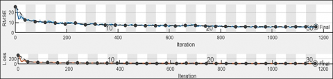
This section summarizes the results of our machine-learning experiments. Figure 4 depicts the training process of a LR model over a series of iterations, plotted against two key metrics: (RMSE) and loss.
In the upper graph, RMSE is quite high initially, a scenario that’s usual since the model begins with randomly initialized parameters. Nonetheless, the decay rate is low, suggesting that the model is showing signs of learning from the data. In the course of iterations, the RMSE becomes stable and converges to a low value, so a conclusion can be drawn that the model’s predictions are moving towards the actual values. RMSE, in general, doesn’t display big changes starting from the middle of iterations. This may indicate that the model used as much information as possible in the training data.
The bottom graph displays the loss, which in LR is the sum of the squared difference between the predicted and actual values, also known as ‘the cost function’. The pattern is quite like RMSE, which has a high value in the beginning and rapidly starts from down and level. Thus, the model tends to get the same set of parameters (weights and biases) that minimize the loss function, and further training doesn’t change its parameters significantly.
Both plots spotlight a "Final" marker, which signifies the ending of the training process. The reason for this could be either once the pre-fixed number of iterations is completed, or the stopping criterion is met, such as a minimum change in RMSE or loss over a pre-fixed number of iterations.
The MSE values obtained by the ML models in the suite of our models endorse the compelling narrative on their respective predictive accuracies in estimating hourly air temperature, as shown in Table 1. (SVR) model with the MSE of 2.9099 turns out to be the most accurate model from our set of models. The SVR kernel trick, especially in the conditions when the RBF kernel is used, allows SVR to capture complex, non-linear patterns in the data that seem to be most effective in this case. It is superior, showing that it is strong enough to deal with the challenging nature of the atmospheric data, which sometimes has nonlinear relationships between predictors and target variables.
Table 1. Model MSE comparison
|
Model |
MSE |
|
Support Vector Regression |
2.9099 |
|
Decision Tree |
3.0613 |
|
Ridge Regression |
4.2541 |
|
Lasso Regression |
4.4651 |
|
Linear Regression |
5.0532 |
Similarly, the DT model shows a low MSE of 3.0613. This aspect indicates that the model’s hierarchical, nonparametric method is enough to capture the data variance pretty well but not as finely as the SVR. Regarding decision trees, their interpretability can be applied to reveal the interaction between the features and the target variable despite the accuracy of prediction with a small loss.
Figure 4. Learning process of LR
The Ridge Regression model yields an MSE of 4.2541, suggesting a moderate fit. The inclusion of L2 regularization helps prevent overfitting, which might be particularly beneficial if the dataset has multicollinearity among predictors. However, the linear nature of Ridge Regression may limit its ability to model more complex relationships in the data, which could explain the higher MSE compared to SVR and Decision Trees.
LSR with an MSE of 4.4651, also imposes regularization, but with an L1 penalty, encouraging sparsity in the model. While it tends to perform feature selection by driving some coefficients to zero, it appears that this property did not translate into higher predictive accuracy in this specific case. This could be due to the loss of informative predictors that are important for capturing the full complexity of the air temperature’s variance.
Lastly, the LR model records an MSE of 5.0532, the highest among the models. Being the simplest model with no regularization or mechanisms to handle nonlinearity, its performance suggests that the relationship between the predictors and air temperature is too complex for a simple linear model to capture accurately.
These results emphasize the importance of choosing the suitable model for the dataset at hand. While simpler models are more interpretable, they may not always capture the underlying complexities of environmental data. Conversely, models that can handle complex relationships and have regularization to prevent overfitting can be more predictive. These insights could guide us in refining these models further or combining them in an ensemble method to leverage their respective strengths.
Table 1 presents a very persuasive story of the predictive accuracy in estimating hourly air temperature is presented by Mean Squared Error (MSE) values obtained from ML models. The SVR model having an MSE of 2.9099 is the most accurate out our suite of models.
SVR with RBF Kernel: SVR also outperforms DT and RF shows the ability to robustly construct a model even in very complex and nonlinear situations. By using the RBF kernel, an SVR is capable of mapping input features to a higher-dimensional space where linear separation between meteorological variables and air temperature exists. This attribute makes SVR a very strong technique when working with the non-stationary time-series data, which is notoriously difficult to predict due to complex interactions between predictors and target variables.
DTR: DTR performs just behind SVR with an MSE of 3.0613. Decision Trees are great for being interpretable, and modeling the variance in data by leveraging a hierarchical way of handling non-linear relationships. However, they suffer from overfitting unless correctly pruned. The interpretability of the model, where interactions are not neglected and can contribute to its high accuracy.
Ridge Regression Model: MSE=4.2541, so fits a little bit better than the previous model The L2 regularization of Ridge Regression is a way to avoid overfitting and works particularly well on data with high multicollinearity amongst the predictors. The linear nature of the model allows it to fit well in case there is a probability distribution, but makes its capabilities quite limited for more complicated relationships hence yielding higher MSE than SVR or Decision Trees.
LSR: L1 regularization is added to minimize the cost function (the MSE in this case) and generate a sparse model while eliminating some of coefficients [7], with an MSE score equivalent to 4.4651. Although beneficial, this feature selection did not lead to greater predictive accuracy (but perhaps partly because it excluded so many informative predictors that are needed to properly model the complexity of air temperature variability).
LR: With a maximum MSE of 5.0532, the simple Linear Regression model (no regularization and no non-linearity) struggled to properly account for all interrelations among predictors air temperature. It means that the complexity of atmospheric data exceeds what a simply linear model could hope to capture.
Interpreting Model Performance Results: The differences in performance between these models illustrate the significance of choosing appropriate model for our dataset. Less complex models such as Linear Regression and Lasso Regression are easier to explain, but they might not discover the hidden patterns of environmental data very well (like random forests). Conversely, SVR is able to catch nonlinear relationships and add regularization techniques due to Decision Trees we can induce that their prediction power is far greater.
The higher performance of models like SVR and Decision Trees can be due to their capacity in modeling non-linear properties which occurs a lot within the atmospheric science data. Air temperature is largely influenced by nonlinear interactions among the variable’s humidity, solar radiation, wind patterns. While simple and interpretable linear models are not able to capture these complexities, which results in poor accuracy.
Lessons and Future Work: Lessons learnt to refine these models individually or combined as ensemble methods depending on the nuances of each model are given in this section. Future work could investigate combining several models in an ensemble to achieve the right balance of prediction accuracy and interpretability, or deeper neural network structures capable of learning more intricate features from atmospheric data.
5.1 Related work comparison
Our selected models show clear advantages, comparing them to the classical time series model ARIMA and other machine-learning approaches, as we validated later on.
Alomar et al. [8] examined 27 classical time series models. Chen et al. (2022) compared the performance of different models, such as ARIMA, and the ML model SVR was found to be better in forecasting daily temperature than ARIMA. These results are in line with our work, where SVR yielded the best precision against traditional time series models due to its ability to represent non-linear relationships better than a standard approach.
Deep Learning Approaches: Ozbek et al. [7] used LSTM to forecast the temperature, and its results were well in short-term periods. Although this study did not specifically evaluate LSTM, the observation that SVR was able to capture complex non-linear patterns corresponds with other deep learning models for handling time series data.
Comparisons across Regions: Studies by Hou et al. [10] and Shin et al. [12] explored advanced models such as the CNN-LSTM and hybrids in each region with great improvements in predictive accuracy. Such studies are particularly relevant useful for scenario like Karak City, as the selection of an appropriate model must consider regional data characteristics. Incorporating these hybrid models could potentially enhance the accuracy of our findings using SVR.
Data sample size & feature engineering: Our dataset from the Dead Sea area has a large set of meteorological factors at high resolution, which stresses dedicated data. The approach is like that applied to detailed datasets in Kajewska-Szkudlarek [9] for predicting heating and cooling degree hours, stressing the importance of feature engineering as a tool for improving model performance.
Altogether, these findings corroborate the case for ML approaches but are not dissimilar to conclusions from work in other countries that stress optimal model selection should be sensitive to differences in climatic dynamics and data quality when applied elsewhere.
The novelty of this research is to use ML models effectively for predicting the hourly atmospheric air temperature (AAT) in Karak City, Jordan. Using a highly enriched dataset and stringent preprocessing, we tested multiple prediction models with Support Vector Regression (SVR) using RBF Kernel yielding the highest accuracy reflecting inherent dynamical changes of most climatic data.
This research sheds light on the theoretical progression in environmental prediction demonstrating that ML models, especially SVR performed much better than linear multivariate regression model to capture non-linear and complex associations inherit in atmospheric data. This aspect adds to an evolving picture of how ML has benefitted climatology.
The study highlights the ways in which ML can deliver practical improvements to regional temperature predictions. Improved forecasts could have large applications in agriculture, the urban sector and disaster management, thereby providing decision makers with valuable tools to effectively utilize resources seamlessly for weather resilient planning.
The novelty of this study could be explained in terms that it is a tailored application data with the ML models to local climatic dynamics which are important in understanding world climate variability but has fewer case studies where global information processing was not used.
6.1 Future work
Future work will be pursued in following aspects:
[1] Cobaner, M., Citakoglu, H., Kisi, O., Haktanir, T. (2014). Estimation of mean monthly air temperatures in Turkey. Computers and Electronics in Agriculture, 109: 71-79. https://doi.org/10.1016/j.compag.2014.09.007
[2] Venkadesh, S., Hoogenboom, G., Potter, W., McClendon, R. (2013). A genetic algorithm to refine input data selection for air temperature prediction using artificial neural networks. Applied Soft Computing, 13(5): 2253-2260. https://doi.org/10.1016/j.asoc.2013.02.003
[3] Zahroh, S., Hidayat, Y., Pontoh, R.S., Santoso, A., Sukono, F., Bon, A. (2019). Modeling and forecasting daily temperature in Bandung. In Proceedings of the International Conference on Industrial Engineering and Operations Management, pp. 406-412.
[4] Prodhan, F.A., Zhang, J., Sharma, T.P.P., Nanzad, L., Zhang, D., Seka, A.M., Ahmed, N., Hasan, S.S., Hoque, M.Z., Mohana, H.P. (2022). Projection of future drought and its impact on simulated crop yield over South Asia using ensemble machine learning approach. Science of the Total Environment, 807: 151029. https://doi.org/10.1016/j.scitotenv.2021.151029
[5] Aghelpour, P., Mohammadi, B., Mehdizadeh, S., Bahrami-Pichaghchi, H., Duan, Z. (2021). A novel hybrid dragonfly optimization algorithm for agricultural drought prediction. Stochastic Environmental Research and Risk Assessment, 35(12): 2459-2477. https://doi.org/10.1007/s00477-021-02011-2
[6] Dikshit, A., Pradhan, B., Huete, A. (2021). An improved SPEI drought forecasting approach using the long short-term memory neural network. Journal of Environmental Management, 283: 111979. https://doi.org/10.1016/j.jenvman.2021.111979
[7] Ozbek, A., Sekertekin, A., Bilgili, M., Arslan, N. (2021). Prediction of 10-min, hourly, and daily atmospheric air temperature: Comparison of LSTM, ANFIS-FCM, and ARMA. Arabian Journal of Geosciences, 14: 622. https://doi.org/10.1007/S12517-021-06982-Y
[8] Alomar, M.K., Khaleel, F., Aljumaily, M.M., Masood, A., Razali, S.F.M., AlSaadi, M.A., AlAnsari, N., Hameed, M.M. (2022). Data-driven models for atmospheric air temperature forecasting at a continental climate region. PLoS ONE, 17(11): e0277079. https://doi.org/10.1371/journal.pone.0277079
[9] Kajewska-Szkudlarek, J. (2023). Predictive modelling of heating and cooling degree hour indexes for residential buildings based on outdoor air temperature variability. Scientific Reports, 13: 1-10. https://doi.org/10.1038/s41598-023-44380-4
[10] Hou, J., Wang, Y., Zhou, J., Tian, Q. (2022). Prediction of hourly air temperature based on CNN–LSTM. Geomatics, Natural Hazards and Risk, 13(1): 1962-1986. https://doi.org/10.1080/19475705.2022.2102942
[11] Astsatryan, H., Grigoryan, H., Poghosyan, A., Abrahamyan, R., Asmaryan, S., Muradyan, V., Tepanosyan, G., Guigoz, Y., Giuliani, G. (2021). Air temperature forecasting using artificial neural network for Ararat valley. Earth Science Informatics, 14: 711-722. https://doi.org/10.1007/s12145-021-00583-9
[12] Shin, J.Y., Kim, K.R., Ha, J.C. (2020). Seasonal forecasting of daily mean air temperatures using a coupled global climate model and machine learning algorithm for field-scale agricultural management. Agricultural and Forest Meteorology, 281: 107858. https://doi.org/10.1016/j.agrformet.2019.107858
[13] Bellido-Jiménez, J.A., Estévez Gualda, J., García-Marín, A.P. (2021). Assessing new intradaily temperature-based machine learning models to outperform solar radiation predictions in different conditions. Applied Energy, 298: 117211. https://doi.org/10.1016/j.apenergy.2021.117211
[14] Cho, D., Yoo, C., Im, J., Cha, D.H. (2020). Comparative assessment of various machine learning-based bias correction methods for numerical weather prediction model forecasts of extreme air temperatures in urban areas. Earth and Space Science, 7(3): e2019EA000740. https://doi.org/10.1029/2019EA000740
[15] Ferreira, L.B., da Cunha, F.F. (2020). New approach to estimate daily reference evapotranspiration based on hourly temperature and relative humidity using machine learning and deep learning. Agricultural Water Management, 234: 106113. https://doi.org/10.1016/j.agwat.2020.106113
[16] Tabrizi, S.E., Xiao, K., Van Griensven Thé, J., Saad, M., Farghaly, H., Yang, S.X., Gharabaghi, B. (2021). Hourly road pavement surface temperature forecasting using deep learning models. Journal of Hydrology, 603: 126877. https://doi.org/10.1016/j.jhydrol.2021.126877
[17] Jordan, M.I., Mitchell, T.M. (2015). Machine learning: Trends, perspectives, and prospects. Science, 349(6245): 255-260. https://doi.org/10.1126/science.aaa8415
[18] Famili, A., Shen, W.M., Weber, R., Simoudis, E. (1997). Data preprocessing and intelligent data analysis. Intelligent Data Analysis, 1(1): 3-23. https://doi.org/10.3233/IDA-1997-1102
[19] Zhang, F., O’Donnell, L.J. (2020). Support vector regression. In Machine Learning, pp. 123-140. https://doi.org/10.1016/B978-0-12-815739-8.00007-9
[20] Kingsford, C., Salzberg, S.L. (2008). What are decision trees? Nature Biotechnology, 26(9): 1011-1013. https://doi.org/10.1038/nbt0908-1011
[21] McDonald, G.C. (2009). Ridge regression. Wiley Interdisciplinary Reviews: Computational Statistics, 1(1): 93-100. https://doi.org/10.1002/wics.14
[22] Ranstam, J., Cook, J.A. (2018). Lasso regression. British Journal of Surgery, 105(10): 1348.
[23] Su, X., Yan, X., Tsai, C.L. (2012). Linear regression. Wiley Interdisciplinary Reviews: Computational Statistics, 4(3): 275-294. https://doi.org/10.1002/wics.1198
[24] Chicco, D., Warrens, M.J., Jurman, G. (2021). The coefficient of determination R-squared is more informative than SMAPE, MAE, MAPE, MSE and RMSE in regression analysis evaluation. PeerJ Computer Science, 7: e623. https://doi.org/10.7717/peerj-cs.623