Francesca Vecchi*![]() | Umberto Berardi
| Umberto Berardi![]() | Guglielmina Mutani
| Guglielmina Mutani![]()
This article is part of the Special Issue 8th AIGE/IIETA International conference and 18th AIGE Conference
© 2023 IIETA. This article is published by IIETA and is licensed under the CC BY 4.0 license (http://creativecommons.org/licenses/by/4.0/).
OPEN ACCESS
Decarbonisation policies are often implemented in cities through the promotion of rooftop solar resources. However, urban solar assessments need to identify favourable locations and appropriate sizing to effectively support these strategies. This research aims to estimate the potential for photovoltaic (PV) systems in a dense urban context, as a basis for future policy support. The downtown district of Toronto, Ontario (Canada) is examined as a case study using the 2030 online platform. This work adopts a multi-scalar methodology to model the potential of roof-mounted PV systems for the main residential archetypes. An urban-scale GIS-LiDAR assessment, informed by environmental criteria, is followed by a block-level optimization using URBANopt, which considers energy and economic parameters. The rooftop GIS-based analysis estimates that up to 20% of electricity consumption for detached houses could be satisfied, primarily in the summer, and 5% for apartment buildings. Optimization with URBANopt shows that solar collective configurations can provide significant benefits to users, primarily in terms of economics. When optimization is performed by clusters for each block, the benefits over single-building analysis are evident, particularly in reducing lifecycle costs. In the selected case study, polycrystalline panels with net metering can achieve self-sufficiency levels ranging from 18% to 41% for residential blocks. This study confirms that solar PV systems can increase local production, reduce grid energy dependency, and support energy communities.
solar assessment, GIS, energy community, urban analysis, solar pathways, self-sufficiency
In 2021, building operations accounted for approximately 27% of total emissions in the energy sector and almost one-third of global final energy consumption, primarily from residential stock [1]. Developing countries require effective policies to manage energy supply expansion to new areas. However, actions in the US and EU have not effectively reduced energy consumption with building regulations [2]. Canada still reports one of the highest per-capita electricity consumptions globally, despite a 7% decrease between 2009 and 2019 [3]. According to the 2016 Pan-Canadian Framework on Clean Growth and Climate Change [4], ambitious goals for 2030 include cutting energy consumption by 600 PJ by tightening efficiency standards and codes for buildings, and achieving 90% electricity production from non-emitting renewable resources. In line with this vision, Ontario became the first jurisdiction in North America to completely phase out coal-fired electricity generation in 2015 [5].
Regional and urban policies have been progressively aimed at reducing building energy demand while increasing local renewable energy production. This transition to alternative resources is critical to limiting reliance on traditional fuels, which will be exhausted in the coming decades. Projections from IRENA [6] expect a continuous rise in installed renewable power, reducing the impacts of fossil fuels and progressively reaching net-zero targets. Renewables contribute to addressing the concentrated demand in urban areas. Solar photovoltaic (PV) systems have the highest potential for integration into urban micro-generation [7]. PV technology is the most feasible for city installation due to the scarcity of other resources (i.e., hydro or wind), space constraints, and legal restrictions [8].
The evaluation of feasible urban areas for PV installation should favor roof-integrated technologies, as roofs are the best part for solar harvesting in dense cities [8]. However, several factors of roof design affect PV performance, such as slope, surface orientation, shading effects, and obstructions from nearby buildings, vegetation, chimneys, skylights, etc. [9]. PV systems generally operate behind the meter and feed their overproduction into the grid through net-metering schemes or feed-in tariffs [10]. Distributed solar systems can contribute to peak shaving, improve the reliability of electrical provision, and reduce transmission-distribution energy losses due to the proximity of production and consumption points [11]. The perspective is towards collective configurations, such as energy communities (EC), which allow energy sharing and provide both energy and economic benefits for users if effectively designed [12].
The successful implementation of PV systems in buildings necessitates local-based assessments to determine the potential of solar energy in urban contexts, which can vary with urban morphology [13]. Several evaluations have modelled the solar potential on rooftops for this reason. Existing studies have extensively explored roof-PV production for single buildings from technical, economic, and environmental perspectives [14]. Urban-level assessments are primarily based on Geographic Information System (GIS) elaborations, offering a good balance between workflow simplification, quick processing, and detail of results, especially when using Light Detection and Ranging (LiDAR) sources [15]. Some GIS approaches [8] focus more on sunlight and shade obstructions to calculate PV production, while others concentrate on roof typologies [16]. However, these approaches are not feasible for evaluating community-based solar hypotheses at the neighbourhood scale. Collective solar scenarios can identify the economic advantages of sharing resources and production among buildings [17]. Although initially ECs aimed to maximize collective self-consumption and self-sufficiency to achieve multiple environmental and social benefits, current market pressures necessitate the identification of economic objectives [11].
The objective of this work is to develop an integrated framework for multi-scale solar assessments. The results build evaluations to identify potential areas for PV project development and prioritize the allocation of local resources by administrations. City governments play a crucial role in promoting solar diffusion, introducing policy tools, and tailoring state-level regulations [18]. Identifying the most suitable buildings helps prioritize the allocation of local resources for solar installations. The study applies a primarily environmentally oriented GIS-based approach at the urban scale, while a community block-level optimization integrates economic and energy parameters. Both methods are tested on a dense urban context for residential use to support city energy policies. The first part describes the methodology and the main parameters adopted, followed by a short presentation of the central Toronto area case study, known as the TOcore area. The urban GIS assessment is based on a LiDAR Digital Surface Model (DSM), with criteria including slope, exposure, and performance, and distinguishing the main building archetypes. The block-scale optimization investigates the energy-related and economic advantages of PV implementations. Results and their discussion highlight the main contributions and policy implications of residential PV and possibilities for block-scale configurations.
Cities are energy sinks, for which specific evaluations are needed to face energy challenges at different territorial levels. Studies have mostly investigated solar potential in cities with one spatial scale of analysis. Urban-scale studies generally adopt GIS-based methodologies with roof shape standard and performance criteria [8, 19, 20], from which the solar production is estimated for each building. Other research evaluate the aggregation of load profiles by limited clusters of buildings and match technical and economic parameters in the analyses [14, 17]. However, they are not integrated to a wider framework of evaluation for energy planning. Since the solar technology, mainly PV, is the most commonly available renewable in urban contexts and it has been progressively supported by energy policies, new evaluation approaches are needed to understand how integrate installations to the current state. The goal is to provide a multi-scalar solar PV assessment as a support for future city energy planning. While most studies apply only one level of analysis to determine the solar potential, this research integrates two spatial frames and variable level of detail. Techno-environmental and economic aspects are considered for two approaches and scales. The optimal size of PV systems will support self-sufficiency, which is the ratio between self-consumption by local energy production and the total consumption (SC/C).
The first part consists of a solar GIS-based assessment, working on an urban scale for 75 residential blocks. The GIS technique considers only roof portions with optimal exposure and orientation for PV panels, applying local-based criteria. The second part consists of solar optimisations for four blocks using URBANopt. The software integrates Radiance and REopt, which respectively assess the solar output evaluating building dimensions, orientations, and reflections of surrounding objects and calculate the techno-financially optimal size of the system. URBANopt applies both financial and technical requirements and can perform aggregated and stand-alone scenarios. The level of detail and type of parameters vary with the frame of analysis necessary for energy policies to assess the solar potential.
2.1 Assessment of photovoltaic potential at urban scale
A GIS-based methodology identifies the optimal PV areas on which the electricity produced for each rooftop is calculated. The optimal roof surfaces to install PV are selected using criteria for exposure, slope, and minimum performance preferable for the case study. The GIS environment leads to a satisfying level of detail using LiDAR images. LiDAR sources consider natural and anthropic obstructions of the urban environment, which impact on PV production. In ArcGIS licensed software, the Area Solar Radiation (ASR) plugin is launched on the LiDAR-derived DSM (year 2015, 0.5 × 0.5m) selecting the TOcore area. The selected parameters are: time configuration as year with monthly interval; year 2017; 1-hour interval with outputs for each interval; 16 azimuth directions used when calculating the viewshed; diffuse model types with standard overcast sky. The diffuse solar ratio (DR) and transmissivity (T) inserted in the ASR tool are retrieved respectively from the PVGIS portal [21] and Meteonorm software, with coordinates of the Toronto city hall. The values of DR and T derived from two websites (PVGIS and Meteonorm) are grouped based on the average daily hours of light per month. Four intervals are defined using the standard deviation (σ) from the average number of hours (μh) of light for all months. In the four intervals (μh + σ, μh + 2σ, μh – σ and μh - 2σ), the mean DR and T are inserted to launch the ASR simulations. ASR results are then transformed with “Raster to point” tool and joined by location with the buildings’ polygons, selecting each month from the folder of the respective interval. The grid-code is the monthly solar radiation (Wh/m2), from which the electrical PV production [22] is estimated for each building:
$E=P R \cdot H s \cdot S \cdot n p v$ (1)
where, E = annual produced electricity (kWh/y); PR=system performance ratio (i.e., 0.75), which is the ratio between the actual and the nominal yield, including PV losses. McKenney et al. [23] elaborated spatial models for PV potential in Canada with PR = 0.75. Pelland and Poissant [24] estimated building integrated PV in Canada with the same PR value. Therefore, 0.75 is assumed for this urban solar analysis; Hs = cumulative annual solar radiation (kWh/m2/year); S = net surface of the PV module (m2); ƞpv = energy conversion efficiency of PV modules. A polycrystalline Silicon panel (poly-Si, η = 0.18), is selected, according to the updated efficiencies in 2021 [25].
From the shape file with the ASR output, the optimal areas are identified with techno-environmental constraints. The minimum building footprint surface is 30 m2 and with at least one contiguous pitch with a projected horizontal footprint greater than 10 m2, which is roughly a 1.5 kW system with a 15% efficiency and feasible for residential applications [8, 15]. The area must register at least 800 kWh/m2/y of annual solar radiation [26]. Suitable roof portions have a slope of 45° or less, retrieved from SolarTO platform [26]. The slope is found with the Slope (3D Analyst) tool in GIS and then the slope interval is selected with the Raster Calculator. The optimal tilt angle varies with latitude and PVGIS identified 35° for Toronto. Toronto is located at 43°42' N latitude and 79°24' W longitude. Inclinations equal to latitude generally produce more electricity annually, while inclinations greater than the latitude angle have a more constant production but lower annual output [8]. Lower slopes are more productive in summer, while steeper slopes are more productive in winter. Rooftops must face South or South-East for optimal orientation; in particular, for Toronto, PVGIS assesses -2° as optimal azimuth angle. The azimuth identifies the direction which the surface should be at the considered location [8]. The Aspect tool identifies the roof exposure, which classifies surfaces into nine azimuth classes. The Raster calculator then selects only South (157.5-202.5°) and South-East (112.5-157.5°) surfaces. The optimal roof exposures and slopes are in line with a previous study for 10 Canadian cities and 16 Ontario locations [27]. The average optimal tilt angle was found to be 9.6° less than latitude and the average optimal azimuth was found to be 1.9° west of the south. The most performative conditions for panel installation are considered in this study on residential stock. As shown in a previous study [28], the production by less other exposures can contribute to cover the electricity load in other parts of the day and complement the production from the optimal oriented pitches.
From the selection of optimal PV areas, the self-sufficiency (SC/C) is calculated as ratio between used PV output and electrical consumption of each dwelling. The electricity consumption is assessed with two statistical models for appliances-lighting (AL) and space cooling (SC). They are built for Toronto, retrieved from a previous study [29]. The models work on statistical regressions, which relate the main characteristics of the housing stock and the disaggregated electricity consumption retrieved from the 2030 Platform [30]. The regressions return the variables and coefficients which build the equation to estimate the consumptions for each dwelling, reported in Table 1. The article [29] is suggested for a more detailed description of the methodology.
Table 1. Variables and coefficients (coeff.) to perform regression models for AL and SC for each dwelling [29]
|
Variables |
AL Coeff. |
SC Coeff. |
|
Intercept |
26.6283 |
-3.1531 |
|
Number of floors |
-0.6543 |
- |
|
S/V ratio |
22.7825 |
8.6972 |
|
% pre-1980 |
27.8844 |
1.7955 |
|
AL/m2 |
- |
0.065 |
2.2 Photovoltaic optimisation by block
The second solar analysis optimizes PV installations for four residential blocks, using URBANopt. Based on the input data, the software finds the optimal PV configuration which minimizes lifecycle costs (LCCs) for users. The main input data, steps to perform block-level analyses and outputs are summarised in Figure 1.
Figure 1. Input data and steps to optimize PV installations with URBANopt simulations based on Reopt
Solar optimizations start from the current electricity consumption (baseline scenario) simulated by the software. Thermophysical input data for each dwelling type are inserted based on the ASHRAE framework and studies on the local housing stock. Table 2 shows the input characterization of the four residential typologies. Representative building models are selected from ASHRAE templates, namely 2006 International Energy Conservation Code (IECC) version for single-family houses and the Department of Energy (DOE)’s Commercial Reference Building models for multi-family buildings. The prototypes are distinguished by climate zones and updated to new requirements of standards and IECC.
Modelling from the current electricity consumption, URBANopt requires location, performance, and financial inputs to optimize PV installations, both for single building and by block of buildings. The former assumes stand-alone structures, while the latter an aggregation of users toward a community-scale project. Simulations assume grid-connected scenarios for 25 years, which is the standard PV lifetime [8]. Poly-Si module prices are selected for the first quarter of 2020, slightly before disturbances from the COVID-19, from the PVInsight dataset (http://pvinsights.com/). In addition to panel prices, installation costs are retrieved from a recent study by the National Renewable Energy Laboratory (NREL) [31], including mainly its manufacturing, labour costs, and market-related variables. A poly-Si technology represents a compromise between efficiency (η = 0.18), prices (0.177 US$/Wp) and space occupied by each kWp (6.7 m2). The installation costs decrease with larger power installed, considering residential systems with less than 10 kW and commercial up to 250 kW. The installation costs are retrieved from a previous study based on Canada [8] and summarised in Table 3.
Table 2. Characterisation of the four residential types, based on ASHRAE frameworks. Detached = DTC, semidetached = SMDTC, low-rise = LR, high-rise = HR
|
Variable |
DTC |
SMDTC |
LR |
HR |
|
Inhabitants/building |
3 |
5 |
31 |
158 |
|
Roof area/inhabitant (m2) |
48.2 |
52 |
32.1 |
6.7 |
|
Age |
Before 1945 |
Before 1945 |
1946-1960 |
1980-2004 |
|
Roof type |
Gable |
Gable |
Flat |
Flat |
|
Foundation basement |
Basement conditioned |
Basement conditioned |
Ambient |
Ambient |
|
Attic |
Vented |
Vented |
Flat roof |
Flat roof |
|
System type |
Natural gas boiler |
Natural gas boiler |
Natural gas boiler + electric AC |
Natural gas boiler + electric AC |
|
Ceiling (W/(m2K)) |
0.36 |
0.36 |
0.33 |
0.25 |
|
Main walls (W/ (m2K)) |
0.9 |
0.9 |
0.82 |
0.37 |
|
Windows (W/ (m2K)) |
2.56 |
2.56 |
3.56 |
3.33 |
|
Foundation walls (W/(m2K)) |
1.92 |
1.92 |
1.85 |
1.85 |
|
Building type, IECC 2006 |
Single-family detached |
Single-family attached |
Multi-family |
Multi-family |
|
Starting ASHRAE template |
IECC 2006 |
IECC 2006 |
DOE pre-1980 |
DOE 1980-04 |
|
Other sources |
[32, 33] |
[32, 33] |
[34, 35] |
[34, 35] |
Table 3. Installation costs classified by PV system size
|
PV System Size (kW) |
Installation Costs ($/kW) |
|
P ≤ 10 |
2,600 |
|
10 ≤ P ≤ 20 |
2,400 |
|
20 ≤ P ≤ 50 |
2,300 |
|
P ≥ 50 |
2,200 |
Source: [8]
The software also requires the local time-of-use (TOU) tariffs to purchase the electricity and eventual incentives or discount to install PV panels. Indeed, incentives and tax rebates are common to push PV diffusion and face the high initial costs [18]. Other input data are required to model the PV performance. The PV production tends to decline in time and a 0.05% yearly degradation is considered [26, 36]. The PV losses are set at 14%, including soiling, shading, light-induced degradation, wiring [15]. The PV inverter has an efficiency equal to 0.96. A DC-to-AC ratio of 1.2 is assumed as the ratio of the nameplate capacity of the PV modules to the AC rated capacity of the inverters [8, 15]. The PV system requires regular maintenance, evaluated as 20 US$/kW/y [36] for cleaning, administration, and replacement of broken parts.
Toronto is located in the climate zone 5A (cool humid). Average temperatures in winter months are around and below 0℃ while summers are warmer, with rising temperature projections [37]. For 2017, the monthly solar irradiation peaks in June and July, when daylight period is longer. Maximum temperatures are one month later based on PVGIS.
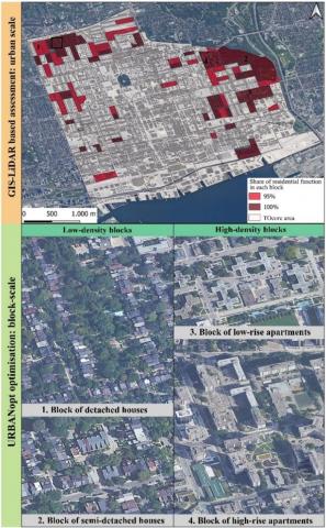
The case study is the central area of the city (Figure 2), which is studied by the 2030 Platform [30]. The online tool provides an energy-consumption benchmarking by block scale and by building function. However, it totally lacks a solar section to estimate local production despite the presence of new city policies for the diffusion of solar PV technology.
Figure 2. Residential blocks in the TOcore area (above), and four blocks by archetypes (below) selected for the two solar evaluations. The bold rectangle in the TOcore highlights the Annex zone selected for Figure 3
Considering this lack, the study provides a solar evaluation for residential buildings, based on two scales of analysis (Figure 2). The first GIS-based approach is at the urban level for the 75 residential blocks of the city centre. Each block has 95% to 100% gross floor area (GFA) occupied by the residential function, based on results of the Platform. The second optimisation is at the block scale, selecting four of these residential areas, one for each dwelling type and in the different downtown neighbourhoods. Four residential types are distinguished for the Canadian context: detached (no shared walls, 2 or 3 floors), semi-detached (at least, one shared wall), low-rise (multiple units with less than 5 floors), and high-rise apartments (multiple units with 5 or more storeys). For the selected residential stock, detached houses have an average S/V ratio (m2/m3) equal to 0.71, semi-detached to 0.53, low-rise apartments to 0.34, while the lowest for high-rises, equal to 0.26.
Table 4. TOU rates by the Toronto hydro electric system, residential TOU tariffs
|
Time of the Day |
Weekdays Summer |
Weekdays Winter |
Weekends, Holidays |
Tariff (US$/kW) |
|
Off-peak |
7 p.m. to 7 a.m. |
7 p.m. to 7 a.m. |
All day |
0.065 |
|
Mid-peak |
7 to 11 a.m. and 5 to 7 p.m. |
11 a.m. to 5 p.m. |
- |
0.095 |
|
On-peak |
11 a.m. to 5 p.m. |
7 to 11 a.m. and 5 to 7 p.m. |
- |
0.132 |
The considered area is served by the Toronto Hydro Electric System, which applies the same time-of-use (TOU) rates for electricity purchased and sold to the grid as shown in Table 4. Indeed, PV scenarios with URBANopt are performed with net-metering, which is an arrangement between customers and the local distribution operator. The customer generates electricity from renewable sources and remains connected to the main grid. On-peak tariffs apply to the central hours of the day when solar radiation is higher and demand pressure on the grid is concentrated. More widespread solar production could reduce the higher costs of electricity purchased in most demanding fractions of the day. The solar overproduction can be sold to the main network and receive a credit in electricity bill to carry over up to 12 months, according to the Ontario Regulation 541/05. Net metering in Ontario was limited to only one user until the Ontario Regulation 679/21, applied for community demonstration projects up to 10 MW.
The Canadian Government also provides for the residential sector the Greener Homes Grant, which is equal to $1,000 \$ / \mathrm{kW}$ up to $5,000 \$$ for detached and semidetached houses and up to $20,000 \$$ for multi-unit residential buildings [39]. It is modelled in the analysis as one solution at the beginning of the lifetime and one grant is considered for each building, according to the maximum coverable investments.
4.1 GIS-based photovoltaic potential on rooftops
The evaluation of incident solar radiation and of the potential production by roof-integrated PV considers the TOcore area for 2,449 residential buildings. The available roof surface is 1,355,902.5 m2. GIS solar simulations are performed monthly to account for the varying lengths of daylight and atmospheric characteristics. The year 2017 was chosen in accordance with the data of the Toronto Platform, which were measured in 2017. Table 5 shows the monthly components of diffuse to global radiation (DR), the Linke Turbidity factor (TL), and the atmosphere transmissivity (T) (see Paragraph 0).
Solar radiation depends on parameters, such as the geographical morphology, density of human activities and pollution levels. The latter contributes to the atmosphere turbidity (considered by the Linke turbidity factor (TL), equal to 1 for perfectly transparent atmosphere) which follows the trend of transmissivity. Higher diffuse ratio is registered from November to January due to the radiation share scattered by atmospheric constituents, as clouds and dust. Indeed, more cloudy days are in winter and autumn, while in densely urbanised areas also pollution particles can contribute to increase scattering effects. On the other hand, the transmissivity is higher in summer months, with a lower diffuse component.
The GIS-based methodology identifies the optimal roof sections, with orientation, slope, and performance criteria. Figure 3 summarises the main steps of the GIS-based methodology. Firstly, it shows the spatial distribution of solar radiation values for winter and summer from the Area Solar Radiation tool. Roof solar profiles are launched on the LiDAR DSM which includes all natural and artificial shading devices impacting PV performance, as the presence of surrounding structures and vegetation.
Table 5. Solar parameters for ASR plugin
|
Months |
DR |
TL |
T |
|
December |
0.52 |
2.6 |
0.34 |
|
January |
0.55 |
2.55 |
0.31 |
|
November |
0.49 |
2.68 |
0.36 |
|
February |
0.44 |
2.83 |
0.43 |
|
October |
0.37 |
3.07 |
0.49 |
|
March |
0.42 |
2.93 |
0.49 |
|
September |
0.24 |
3.16 |
0.61 |
|
April |
0.36 |
3.34 |
0.58 |
|
August |
0.31 |
3.39 |
0.62 |
|
May |
0.36 |
3.56 |
0.60 |
|
July |
0.32 |
3.59 |
0.63 |
|
June |
0.30 |
3.68 |
0.65 |
Source: PVGIS portal [21] and Meteonorm software
The selected roof portions significantly vary and impact the total PV potential for each building. Indeed, maximum values for summer months are more than three times higher than in winter for the same roof areas. Higher output from the ASR tool is register for South-oriented pitches. Figure 4 summarises the share of roof pitches for each orientation, within 45° slope and the mean yearly irradiation. It is confirmed that pitches to South and SE orientation have higher average annual irradiation. They respectively covered 14.2% and 10.6% of the overall roof area and are mostly included in 45° tilt angle. East and West-oriented portions cover 15% and 14.7% of the overall roof areas, but only a limited portion is within 45° slope. In case of steeper slope of the panels, they can cover additional electricity needs although radiation conditions are less performative.
The sum of all the optimal areas by exposure, orientation and performance criteria is equal to 92,067 m2 for the 75 residential blocks, with 40.8 m2 on average for each roof.
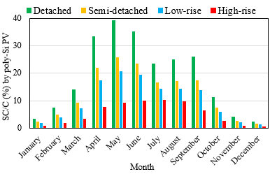
For selected areas, the total PV production is calculated using the Eq. (1) with the selected efficiency. The solar production on rooftops is then related to the electricity consumption for each residential building [29] to obtain the self-sufficiency. Figure 5 reports the monthly variation of self-sufficiency distinguished by residential typologies.
The electricity consumption satisfied by PV production diminishes reducing the S/V ratio and the technology efficiency. Surfaces are more extended for detached and semi-detached dwellings, with an average available area of 18.7 m2 and 38 m2 per building. Based on the statistical models, detached have an average AL and SC consumption respectively of 67.2 kWh/m2/y and 9.1 kWh/m2/y, while semi-detached of 62.9 kWh/m2/y and 7.3 kWh/m2/y. AL and SC intensities are lower for multi-family dwellings, equal to 51.5 kWh/m2/y and 4.7 kWh/m2/y for low-rises and 42.1 kWh/m2/y and 2.9 kWh/m2/y for high-rises. Low-rises and high-rises have an average suitable roof area to install PV of 89.6 m2 and 146.7 m2 but higher number of users and overall building demand. This is confirmed by the average PV surface for each inhabitant, which is 2.8 m2 and 1.7 m2 for low- and high-rises respectively, whereas 4.8 m2 and 3.7 m2 for detached and semi-detached dwellings. PV production on apartment blocks covers a limited percentage (5.1%) of consumed electricity because of the discrepancy between the available roof area and the total demand. The share of electricity satisfied by poly-Si by building type does not exceed 40% per month, with a peak of 39.4% in May for detached houses. In winter, the production can cover less than 10% of the electricity demand in all cases. More potential results from low-density housing, while low-rise and high-rise buildings have peaks of 20.7% in May and 14% in June.
Figure 3. Steps to identify the optimal areas to install PV on GIS. Results are shown for dwelling roofs for some clusters in the Annex area, identified in Figure 2
Figure 4. Roof pitches by orientation, with share of occupied roof areas and average yearly radiation for each m2
Figure 5. Monthly self-sufficiency using PV with optimal location, by residential archetype in Tocore
4.2 Single building and community-based optimisation
The next step of the analysis is optimising PV by residential blocks, considering installation and economic parameters. The aim is to reduce LCCs on a 25-year period, increasing energy locally produced. Four residential blocks are selected one for each typology, or rather detached, semi-detached, low-rises, and high-rise apartments. Each block is optimised by single building and as a cluster with URBANopt to identify energy and economic differences. Table 6 and Table 7 show results for energy aspects (system size, SC/P and SC/C) and Table 8 for financial indicators (lifecycle costs and revenues) with distinction for the two configurations. The two energy indicators are referred to one-year simulation with hourly temporal resolution, using the consumption and PV production calculated.
As shown in Table 7, the size of the PV system is slightly bigger for community-based scenarios. The difference ranges between less than 1 kW for detached houses and about 36 kW for low rises. The slightly bigger system increases the level of self-sufficiency for one year, from +0.3% for detached to +1.6% for high-rise apartments. The SC/C ranges between 18.1% for high-rises and 41.4% for low-rise apartments, which reaches the highest independence from the main grid. Self-consumption is more variable between the two hypotheses because it depends on the amount of energy sold to the grid and locally consumed.
Table 6. Energy-related results for optimisation by single buildings (feature optimization). Size of the optimised system, SC/P = self-consumption, SC/C = self-sufficiency
|
Res. Blocks |
Size (kW) |
SC/P (%) |
SC/C (%) |
|
Detached |
581.9 |
44.1 |
36.7 |
|
Semidetached |
226.1 |
39.8 |
37.7 |
|
Low-rise |
1,254.6 |
52.7 |
40.8 |
|
High-rise |
835.6 |
92.8 |
16.5 |
Table 7. Energy-related results for optimisation by block of buildings (scenario optimisation). Size of the optimised system, SC/P = self-consumption, SC/C = self-sufficiency
|
Res. Blocks |
Size (kW) |
SC/P (%) |
SC/C (%) |
|
Detached |
582.3 |
44.2 |
36.9 |
|
Semidetached |
238.9 |
38.2 |
38.2 |
|
Low-rise |
1,290.3 |
52 |
41.4 |
|
High-rise |
842.7 |
99.5 |
18.1 |
Table 8. Financial-related results for optimisation by single buildings (feature optimisation, f.o.) and by block of buildings (block optimisation, b.o.). LCC = lifecycle cost and NPV = net present value
|
Res. Blocks |
LCC (kUS$) f. o. |
LCC (kUS$) b. o. |
NPV (kUS$) f. o. |
NPV (kUS$) b. o. |
|
Detached |
1,300 |
925 |
423 |
426 |
|
Semi-detached |
419 |
348 |
113 |
116 |
|
Low-rise |
2,971 |
2,877 |
325 |
341 |
|
High-rise |
8,953 |
8,900 |
216 |
217 |
In the four residential clusters, energy-related benefits are limited between single-building optimisations and collective hypotheses, while economic advantages are predominant. The LCCs on a 25-year span are lower for aggregated scenarios: savings are higher for low-density housing, while more limited for apartments. A reduction of about 28.8% LCCs is registered for detached houses with collective analysis compared to single-building optimisation, while only -0.6% for high-rises. Block-scale optimisations increase revenues (based on the NPV), even if no more than +4.7% compared to installations by single building. However, hypotheses towards ECs need to consider a mix of residential types and building functions to exchange the energy produced locally: detached houses can generally provide a share of electricity for most-consuming high-rise buildings to increase self-sufficiency.
The two solar assessments highlight different PV contribution for each housing type, depending on the approach and parameters adopted. The LiDAR GIS-methodology adopts only criteria for roof configuration and performance to select optimal portions to install PV. The solar radiation on roofs and production vary significantly (see Figure 3) due to self-shading effects by other buildings and obstacles to let the sunlight hits PV panels. Following the selected criteria, the usable surface is only 7% of the total residential roof areas. The 98% of roof portions which are S-SE oriented, within 45° slope and at least 10 m2 have an average radiation above 800 kWh/m2/y. GIS-based evaluations reported a higher covered share of electricity consumption for detached and semi-detached typologies [10]: a 20% maximum self-sufficiency and a monthly covered electricity not higher than 40% for May are identified. The monthly trend of SC/C is higher in May because production is already significant, but space cooling needs are still limited, while they increase in June, July, and August. SC/C is lower for apartment buildings due to the less balanced relation between the total electrical consumption and the optimal roof area.
Other guiding criteria can be used for different load profiles, financially oriented and collective simulations, as performed in URBANopt. The collective optimisations by blocks show slightly higher energy production with remarkable economic benefits. Overall, the economic efficiency covers a key role because it may push the implementation and investors to fund PV projects. Clusters of buildings are more performative and economical than stand-alone installations [14]. Lower LCCs characterise mainly low-density blocks, while they are more limited for clusters of low-rises and high-rises.
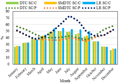
Figure 6. Monthly self-consumption (SC/P, dashed line) and self-sufficiency (SC/C, bars) for detached (DTC), semi-detached (SMDTC) and low-rise (LR) blocks
Figure 7. Hourly electricity consumption and PV production for 4 typical days for one building in the low-rise block
The optimised scenarios with poly-Si and net-metering reach self-sufficiencies between 18% and 41% annually. Figure 6 reports the monthly trend of self-sufficiency and self-consumption for detached, semidetached and low-rise dwellings, which have an annual independence from the grid higher than 35%. The low-rise apartment block shows higher values for both indexes than detached and semi-detached blocks. Indeed, Figure 7 confirms that PV production covers a consistent portion of peak load in the afternoon during summer months, mainly due to space cooling. The self-consumed electricity is also higher for low rises between May and September, with a peak of 73.4%. The self-consumption is lower for low-density housing and overcomes self-sufficiency during winter months, when more than 40% of PV production is instantly consumed. The hourly PV overproduction is purchased from the network with the same TOU tariffs of consumed energy. Tariffs are convenient for customers and exploit the community net metering program, recently introduced by the Ontario Energy Board [40].
Figure 8. Electrical consumption, PV production, self-sufficiency, and self-consumption for the high-rise block
The greatest challenge is for the block of high-rises, where electricity consumption overcomes 500 MWh between June and August. Figure 8 shows the monthly energy profile for the cluster of high-rise apartments. Solar production is almost all instantly consumed due to the high local demand, as confirmed by the self-consumed electricity above 99% for all months. Self-sufficiency is lower in winter due to the limited solar output, whereas space cooling impacts in summer months. Therefore, the maximum self-sufficiency for a financially optimal condition would be 18.1%, with global costs below 9M $US for the whole block.
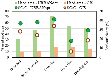
Figure 9 reports a comparison between results with orientation-performance criteria in GIS and URBANopt optimisations, selecting the four residential blocks and adding a hypothesis of mixed residential area. The housing-mix scenario includes one detached, 7 semi-detached houses, 2 low-rises and 4 high-rises and 291 inhabitants overall. The graph reports the share of roof area assessed and the reached level of self-sufficiency. The optimised results in URBANopt are always larger than the identified areas in GIS, especially for multi-family typologies. The GIS evaluation only considers favourable exposures (S-SE) and slopes (≤ 45°) for PV production. On the other hand, block scale simulations optimise PV panels to minimise LCCs over 25 years and balance local production with building energy consumption.
The values of self-sufficiency are higher for the second approach. The main differences are for semidetached (38.2% vs. 24.1%) and high-rise blocks (18.1% vs. 6.5%). In the mixed residential case, a 30% SC/C with URBANopt methodology would be reached due to the complementarity of different production-consumption loads. The solar energy overproduced by low-density dwellings can be sold to most demanding condominiums. This exchange would be particularly useful in the late afternoon, when the demand of electricity is concentrated, tariffs are more expensive and solar production is higher especially in summer. The housing-mix hypothesis proves the benefits of combining different loads in community-scale projects. Future analyses should match distinct residential typologies and non-residential profiles.
Figure 9. Selected roof areas (columns) by GIS methodology and URBANopt optimisation in the five residential clusters. Based on electricity consumption in URBANopt, level of self-sufficiency (SC/C, dots) reached by each method
Further developments of this methodology can:
improve the process to define housing archetypes in different blocks, using GIS environment. The study by Mohajeri et al. [41] developed a machine learning (ML) procedure to estimate variations of housing capacity in UK. A similar use of these tools can be implemented to classify buildings and extend evaluations at a regional scale. ML capabilities can also extract roof surfaces for solar panels on larger datasets, based on selected criteria;
include other installation conditions for solar panels, considering further exposures and tilt angles. Less performing roof pitches may cover the electricity demand in specific part of the day [28], if their installation is financially feasible in the lifetime;
integrate distinct daily and hourly load profiles in community scenarios, as domestic types, offices, commercial, recreational spaces, to increase local self-sufficiency. A careful energy planning to evaluate the pressures of the fluctuating power supply, especially in case of old energy network.
Assessments at an aggregated level, rather than by single buildings, can bring energy performance and financial benefits, making investments more attractive for users.
Energy models are supporting tools for energy planning, especially in urban contexts where the heterogeneity of energy profiles require flexible analyses. For this study, two approaches and scales assessed PV production and the potential self-sufficiency. The residential stock of the central area of Toronto was chosen, considering four dwelling archetypes. The GIS-based solar analysis identified the optimal roof portions by environmental and performance criteria. From the selected surfaces, more effective solar contribution is in spring and summer, especially for detached houses. Using URBANopt for four blocks, PV optimisations highlighted the economic and energy advantages of clusters modelling. Aggregated assessments showed slightly better energy performance and notable economic benefits, particularly for low-density housing. A more diffused solar production injected in the network may decrease energy costs during peak hours and make electricity less expensive.
Although results are preliminary estimates, the flexibility of the procedure in this study can easily guide policy evaluations. The methodology can be easily replicable in other contexts with local-based criteria. The use of multi-scalar energy assessments allows to vary the frame of analysis accordingly to the scope, from urban to local level. The former can be used when a generalised characterisation of a wider area is needed, while the latter in case of more detailed evaluations for energy and economic aspects. Accordingly, two software allow to obtain variable accuracy. The GIS approach localises consumption and identifies the satisfaction of electricity as an overall urban evaluation. The GIS simulations are useful for policy support to identify at the urban scale the optimal areas, applying environment-related criteria. However, they are inadequate to estimate energy and economic benefits along a lifetime. On the other hand, block-scale optimisations with URBANopt are performed for smaller clusters because of computational efforts and longer elaborations. Main advantage is that they evaluate solar performance by collective configurations, financial benefits, and PV investments rather than large-scale overviews. More detailed results can be useful for inhabitants but especially as a support for administrations to foster community-scale projects where higher self-sufficiency can be achieved.
This should be considered for collective preliminary assessments, which are currently lacking in strategies and incentives for decarbonisation in Toronto. A similar double-scale solar assessment inserted in the Platform would make citizens and policymakers more aware on potential of new technologies. The combination of these elements will lead to new energy configurations at the urban level to support energy planning and increase local self-sufficiency by solar resources.
[1] International Renewable Energy Agency - IEA. (2022). Buildings. https://www.iea.org/reports/buildings, accessed on May 17, 2023.
[2] Berardi, U. (2017). A cross-country comparison of the building energy consumptions and their trends. Resources, Conservation and Recycling, 123(4): 230-241. https://doi.org/10.1016/j.resconrec.2016.03.014
[3] International Energy Agency. (2022). Canada 2022. Energy Policy Review. http://www.iea.org/, accessed on May 20, 2023.
[4] Government of Canada. (2016). Pan-Canadian framework on clean growth and climate change. Canada plan to address climate change and grow the economy. https://www.canada.ca/en/services/environment/weather/climatechange/pan-canadian-framework.html, accessed on Apr. 2, 2023.
[5] Canada Energy Regulator. (2023). Provincial and territorial energy profiles – Canada. https://www.cer-rec.gc.ca/en/data-analysis/energy-markets/provincial-territorial-energy-profiles/provincial-territorial-energy-profiles-canada.html, accessed on Apr. 2, 2023.
[6] International Renewable Energy Agency - IRENA. (2022). Renewable power generation costs in 2021. Report, Abu Dhabi, UAE.
[7] Kammen, D., Sunter, D. (2016). City-integrated renewable energy for urban sustainability. Science, 352(6288): 922-928. https://doi.org/10.1126/science.aad9302
[8] Kouhestani, F., Byrne, J., Johnson, D., Spencer, L., Hazendonk, P., Brown, B. (2019). Evaluating solar energy technical and economic potential on rooftops in an urban setting: The city of Lethbridge, Canada. International Journal of Energy and Environmental Engineering, 10(11): 13-32. https://doi.org/10.1007/s40095-018-0289-1
[9] Odeh, S., Nguyen, T. (2021). Assessment method to identify the potential of rooftop PV systems in the residential districts. Energies, 14(14): 4240-4251. https://doi.org/10.3390/en14144240
[10] Byrd, H., Ho, A., Sharp, B., Kumar-Nair, N. (2013). Measuring the solar potential of a city and its implications for energy policy. Energy Policy, 61(7): 944-952. https://doi.org/10.1016/j.enpol.2013.06.042
[11] Iazzolino, G., Sorrentino, N., Menniti, D., Pinnarelli, A., De Carolis, M., Mendicino, L. (2022). Energy communities and key features emerged from business models review. Energy Policy, 165(4): 112929. https://doi.org/10.1016/j.enpol.2022.112929
[12] Mutani, G., Santantonio, S., Beltramino, S. (2021). Indicators and representation tools to measure the technical-economic feasibility of a renewable energy community. The case study of Villar Pellice (Italy). International Journal of Sustainable Development and Planning, 16(1): 1-11. https://doi.org/10.18280/ijsdp.160101
[13] Todeschi, V., Marocco, P., Mutani, G., Lanzini, A., Santarelli, M. (2021). Towards energy self-consumption and self-sufficiency in urban energy communities. International Journal of Heat and Technology, 39(1): 1-11. https://doi.org/10.18280/ijht.390101
[14] Aghamolaei, R., Haris Shamsi, M., O'Donnell, J. (2020). Feasibility analysis of community-based PV systems for residential districts: A comparison of on-site centralized and distributed PV installations. Renewable Energy, 157(9): 793-808. https://doi.org/10.1016/j.renene.2020.05.024
[15] Gagnon, P., Margolis, R., Melius, J., Philips, C., Elmore, R. (2016). Rooftop solar photovoltaic technical potential in the United States: A detailed assessment - Technical report. National Renewable Energy Laboratory (NREL) - Golden, Colorado. https://doi.org/10.7799/1575064
[16] Hofierka, J., Kanuk, J. (2009). Assessment of photovoltaic potential in urban areas using open-source solar radiation tools. Renewable Energy, 34(10): 2206-2214. https://doi.org/10.1016/j.renene.2009.02.021
[17] Awad, H., Gul, M. (2018). Optimisation of community shared solar application in energy efficient communities. Sustainable Cities and Society, 43(11): 221-237. https://doi.org/10.1016/j.scs.2018.08.029
[18] Li, H., Yi, H.T. (2014). Multilevel governance and deployment of solar PV panels in U.S. cities. Energy Policy, 69(3): 19-27. https://doi.org/10.1016/j.enpol.2014.03.006
[19] Nguyen, H., Pearce, J. (2013). Automated quantification of solar photovoltaic potential in cities. International Review for Spatial Planning and Sustainable Development, 1(1): 46-60. https://doi.org/10.14246/irspsd.1.1_49
[20] Santos, T., Gomes, N., Freire, S., Brito, M., Fonseca, A., Tenedorio, J. (2011). Solar potential analysis in Lisbon using LiDAR data. Solar Energy, 86(1): 283-288. https://doi.org/10.1016/j.solener.2011.09.031
[21] EU Science Hub. (2022). PVGIS Photovoltaic Geographical Information System. https://joint-research-centre.ec.europa.eu/pvgis-photovoltaic-geographical-information-system_en, accessed on Mar. 20, 2023.
[22] Suri, M., Huld, T., Dunlop, H., Ossenbrink, H. (2007). Potential of solar electricity generation in the European Union member states and candidate countries. Solar Energy, 81(10): 1295-1305. https://doi.org/10.1016/j.solener.2006.12.007
[23] McKenney, D., Pelland, S., Poissant, Y., Morris, R., Hutchinson, M., Papadopol, P., Lawrence, K., Campbell, K. (2008). Spatial insolation models for photovoltaic energy in Canada. Solar Energy, 82(11): 1049-1061. https://doi.org/10.1016/j.solener.2008.04.008
[24] Pelland, S., Poissant, Y. (2006). An evaluation of the potential of building integrated photovoltaics in Canada. In 31st Annual Conference of the Solar Energy Society of Canada (SESCI), Montréal, Canada.
[25] Green, A., Dunlop, E.D., Hohl-Ebinger, J., Yoshita, M., Kopidakis, N., Hao, H. (2021). Solar cell efficiency tables (version 59). Progress in Photovoltaics Res Application, 30(1): 3-12. https://doi.org/10.1002/pip.3506
[26] City of Toronto. SolarTO Map. https://www.toronto.ca/services-payments/water-environment/environmental-grants-incentives/solar-to/solarto-map/#location=&lat=&lng=, accessed on Apr. 20, 2023.
[27] Kemery, B., Beausoleil-Morrison, I., Rowlands, I.H. (2012). Optimal PV orientation and geographic dispersion: A study of 10 Canadian cities and 16 Ontario locations. In eSim 2012: The Canadian Conference on Building Simulation, Halifax Nova Scotia.
[28] Mutani, G., Todeschi, V. (2021). Optimization of costs and self-sufficiency for roof integrated photovoltaic technologies on residential buildings. Energies, 14(13): 1-25. https://doi.org/10.3390/en14134018
[29] Vecchi, F., Berardi, U., Mutani, G. (2023). Data driven urban building energy models for the platform of Toronto. Energy Efficiency, 16(26): 1-19. https://doi.org/10.1007/s12053-023-10106-8
[30] Jermyn, D. (2008). Deep energy retrofits: Toronto's urban single family housing stock. MSc thesis. Department of Applied Science, Toronto Metropolitan University, Toronto, Ontario, Canada.
[31] Blaszak, K. (2010). Towards sustainability: prioritizing retrofit options for Toronto's single-family homes. MSc thesis. Department of Applied Science, Toronto Metropolitan University, Toronto, Ontario, Canada.
[32] Touchie, M., Binkley, C., Pressnail, K. (2013). Correlating energy consumption with multi-unit residential building characteristics in the City of Toronto. Energy and Buildings, 66(11): 648-656. https://doi.org/10.1016/j.enbuild.2013.07.068
[33] Alsaadani, S., Roque, M., Trinh, K., Fung, A., Straka, V. (2016). An overview of research projects investigating energy consumption in Multi-Unit residential buildings in Toronto. Sixth Asian Conference on Sustainability, Energy and the Environment, Kobe, Japan.
[34] Fu, R., Fieldman, D., Margolis, R. (2018). U.S. Solar photovoltaic system cost benchmark: Q1 2018. National Renewable Energy Laboratory (NREL), Golden, Colorado. https://doi.org/10.7799/1503848
[35] Jordan, D., Kurtz, S., VanSant, K., Newmiller, J. (2016). Compendium of photovoltaic degradation rates. Progress in Photovoltaics: Research and Applications, 24(7): 978-989. https://doi.org/10.1002/pip.2744
[36] Environment and Climate Change Canada. (2021). Temperature Change in Canada: Canadian Environmental Sustainability Indicators. https://www.canada.ca/en/environment-climate-change/services/environmental-indicators/temperature-chang, accessed on Mar. 2, 2023.
[37] 2030 District. (2020). Toronto 2030 Platform. https://www.toronto2030platform.ca/, accessed on Feb. 20, 2023.
[38] National Renewable Energy Laboratory - NREL. (2017). International utility rate database OpenEI. https://apps.openei.org/IURDB/?country=CAN§ors%5B%5D=Residential&service_type=&is_default=&search=, accessed on Feb. 20, 2023.
[39] Government of Canada. (2022). Eligible retrofits and grant amounts. https://www.nrcan.gc.ca/energy-efficiency/homes/canada-greener-homes-grant/start-your-energy-efficient-retrofits/plan-document-and-complete-your-home-retrofits/eligible-grants-for-my-home-retrofit/23504, accessed on Mar. 15, 2023.
[40] Ontario Energy Board. (1998). Ontario Regulation 679/21 - Community net metering projects. S.O. 1998 c. 15, Sched. B.
[41] Mohajeri, N., Walch, A., Smith, A., Gudmundsson, A., Assouline, D., Russell, T., Hall, J. (2023). A machine learning methodology to quantify the potential of urban densification in the Oxford-Cambridge Arc, United Kingdom. Sustainable Cities and Society, 92(5): 104451. https://doi.org/10.1016/j.scs.2023.104451