Tahir Mahmood* | Sosan Shireen | Muhammad Mumtaz
© 2021 IIETA. This article is published by IIETA and is licensed under the CC BY 4.0 license (http://creativecommons.org/licenses/by/4.0/).
OPEN ACCESS
Increase in the greenhouse gases (GHGs) such as carbon dioxide (CO2) are responsible for environmental problems like global warming and climate change. This study applies the Stochastic Impact by Regression on Population, Affluence and Technology (STIRPAT) framework to analyse the impact of population, economic growth, economic development, urbanization, and energy use on per capita carbon emissions for India and China. Environmental Kuznets Curve (EKC) hypothesis is also tested within the STIRPAT framework. A time series analysis is done from 1980 to 2019 for China and India. Through application of Auto Regressive Distributed Lag (ARDL) Model, we found the existence of EKC for China and India. Results further show that population and energy use is positively related to CO2 discharges. In case of India, urbanization positively affects CO2 discharges whereas for China our findings show that urbanization helps in reducing CO2 discharges. However, domestic loan to private sector has resulted in environmental degradation in case of both countries.
environmental Kuznets curve, financial development, greenhouse gases urbanization
Greenhouse gases (GHGs) have an extremely critical role in maintaining the earth’s temperature which is important for human life to existThese gases mainly consist of carbon dioxide (), methane, ozone, nitrous oxide, and water vapours. On the heels of industrial revolution, many activities have involved high level of fossil fuel consumption such as urbanization. Expansion of industrialization amplified GHGs and led to global warming and climate change (IPCC, 2007).
Deforestation and the burning of fossil fuels like oil, gas and, coal for generating electricity which are needed for transportation, household and industrial uses have increased GHGs emissions [2]. The increase in GHGs is considered to be the greatest environmental issue faced by the world today [3]. This human induced change in the climate has caused the global annual average temperature of land and ocean to rise by 1.5°F or 0.8°C during the period of 1880 to 2012 [4].
Over the past few years, policymakers, environmentalists, and economists have shifted their attention towards the global environmental issues particularly towards the problems generated due to economic growth or economic development The Environmental Kuznets Curve (EKC) which is based on the work of has very important part in explaining the association among environment and economic growth which suggests that environmental growth has got a reversed U-shaped relation. The EKC exists in certain cases and under certain circumstances.
While studying environment growth relationship, it is significant to study the role of financial development because it plays an extremely important role in economic growth. Countries having efficient financial management system use financial resources effectively, with scarce financial resources. This system would be favourable for the progress of economic development [7].
The financial development-Carbon emission nexus discussed in two strands: One school of thought explains that the carbon emissions increase through financial development. Developed financial markets reduce the financing costs to finance new projects and buy new equipment’s which increased the level of energy hence increase carbon emissions [8]. Zhang et al. [9] argues that financial intermediation increases the buying power of consumer and they can purchase air conditioner, cars, washing machines etc. consuming high energy that leads to affect environment quality negatively. The other school of thought is evident to increase environment quality through financial development. Frankel and Romer [10] argue that financial development attracts foreign direct investment which increase the research and development activities, leads toward better quality of environment. Institutional quality plays an important role in improving environment quality and carbon dioxide emission decreases in the countries where institutions are strong [8, 11].
Before 1978, The People’s Bank of China was the single bank which was operating as central and commercial bank in China but subsequently in 1984; four big state held commercial banks were established who acted as the lender of money to the state owned businesses in construction, rural banking business, foreign trade and national economy, commercial sector and urban industrial activities. As the financial sector began to expand in 1980’s, new banks, financial institutions, and even non-banking financial institutions were established. Moreover, the foreign banks also entered in China in 1990s. In 1990 and 1991 Shanghai Stock Exchange along with Shenzhen Stock Exchange were established. After China’s membership of world health organization during 2001, financial liberalization took place in real terms. Restrictions on interest rates and loans were reduced. China Banking Regularity Commission was established as a supervising body in 2003. By 2006, due to relaxing restrictions on foreign banks, 242 offices were established by 223 foreign banks from 42 countries [12]. In India, financial reforms have taken since 1990’s which have led to the expansion of the financial sector.
Besides these, many other variables are there which have immense effect on environment. Urbanization is a vital aspect which effects carbon emissions. According to the world urbanization prospects (2014) the world has rapidly urbanized. The findings of the report show that 66% population of the world will be living in cities up to 2050. Prediction is that by 2050 larger than 80% countries of the world will be half urban. So the process of urbanization needs to be done in a planned and controlled manner. The problems that can arise due to unplanned and over urbanisation are urban poverty, lack of provision of basic services like access to electricity or sanitation, air pollution, political unrest and violence [13, 14].
The quality of environment decreases by increasing the level of urbanization in different economies with poor environmental concern and awareness. Urbanization still plays an important role and increase across the globe, as people shift from rural areas to urban areas in search of better social environment and social security. Urbanization Promotes productivity, create more wealth and creativity to redesign different structures which would be useful for economic gain. However, the increase in urbanization leads towards consuming high energy leads towards high carbon emissions [15]. In addition, it can be noted that china’s quick urbanization leads to increase high energy demand. The large scale construction of buildings and infrastructures in urban areas need to use large amount of cement, iron and steel, which is hard to import completely, and has to be produced locally. Due to this, it posture great pressure on environmental quality [9].
On the bases of population growth rate Zhang et al. [16] explained that from 1978 to 1988 the rate at which urban population grew was much higher than the rate at which the overall population grew. The total population grew at 1.29% per annum while the urban population grew at the rate of 3.79 %. In addition, from 1978- 1999 the overall increase in the rate of total population was 1.44% while the urban population growth reached to 4.97%. From 1978 to 1999 almost 174 million people migrated to urban areas [17].
On the contrary, the Indian urban population has increased from 18% to 31.2% from 1960 to 2011 According to 2007’s United Nations State of World Population Report about 40.8% of Indian population will be living in urban areas by 2030.
The outcomes of one research cannot be employed over all countries or for all cases. Therefore, each study is unique and different from the other on the basis of the indicators selected, methodology, and data selection and it gives different results even for the same country [19]. This uniqueness of this research method makes it even broader and more interesting. This study examines the impact of urbanization and economic development on the EKC by looking the cases of China and India. The organization of the paper is as follows. Literature review is presented in Section 2. Data and methodology for the study has been discussed in Section 3. The estimation outcomes are presented in Section 4. Section 5 is the conclusion of the study.
We divide the existing literature into three sections which explained the relationship of Economic growth, financial development, Urbanization with carbon emissions.
Kuznet in 1955 suggested that income inequality and per capita income had a reversed U-shaped affiliation which is acknowledged as the Kuznets curve. Grossman and Krueger [20] in 1991 used this as a base model to empirically test the environmental and economic development relationship and suggested that development and environment had a reversed U-shaped relation because at early stages of growth the level of pollution increases but after achieving a certain level of income any addition in the income causes a decline in the emissions. Panayoutu [21] termed this inverted U-shaped curve as EKC. Later Seldon and Song [22], and Grossman & Krueger [23] also proved this reversed U-shaped association among degradation of environment and economic growth.
2.1 Economic growth and carbon emissions
In the early phase of growth, the use of energy due to inefficient methods of production high levels of emissions take place because there is zero demand for the environmental friendly products. However, on achievement of a definite income level, which is shown through the turning point on the curve, the environmental quality starts to improve due to several reasons such as increase in the demand for the eco-friendly technological methods, changes in the input mix increased demand for environmental friendly products which ultimately transforms the economy into green economy [24]. This reversed U-shape of the EKC also depicts a change in society’s consumption behaviour over time with the increase in the society’s level of income [25].
When a society is experiencing growth it moves from agriculture sector to industrial sector becoming energy intensive so it generates more pollution [26]. However, Stern 2004 further states that economic growth keeps occurring and the economy will again shift from industrial to services sector which produces pollution less than the industrial sector so the overall level of pollution declines thus forming a reversed U-shaped EKC.
The existence of the EKC for each country, and even within a country, depends on various factors such as the variable selected as an indicator of environment or growth or the methodology applied. China and India both are fastest growing economies. Recent literature encourages the presence of the EKC for China [27]. On the other hand, Alam et al. [28] denies the existence of the EKC for China in the short term but accepts its presence for long term, while Pal and Mitra [29] reject the EKC hypothesis for China. In India’s case both reject the occurrence of the EKC, but Kanjilal and Ghosh [30] and Boutabba [31] confirmed the existence of EKC for India.
2.2 Financial development and carbon emissions
The development of the financial sector plays a vital part in the economic expansion of a country. In order to explain the link between environment and financial development, Frankel and Romer [10] suggested that a well-functioning financial system attracts more FDI and enhances research and development which causes economic growth and influence environmental quality. A well-established financial institution provides funds for projects related to environment at lower costs [32]. Carbon trading also requires a healthy execution of financial system as the programs conducted by the regulatory authorities are directly related to the financial markets [33]. Furthermore, Birdsall and Wheeler [34] and King and Levine [35] believe that financial development may lead to technological advancements which will play a key part in the improvement of the environment. Frankel and Romer [10] also agree that financial development will lead to the adaptation of eco-friendly technological methods which will help in lowering pollution. Different studies show that financial development has not caused pollution rather it has helped in improving the environmental quality [36].
On the contrary, Jenson [37] suggests that financial development attracts FDI and as these foreign investments increase as it causes the expansion of industrial activities which results in more pollution. Furthermore, Zhang [38] argues that as the financial sector develops it may provide easier financing facilities to the listed companies in the financial markets which will result in more energy demanding projects and will lead to greater CO2 emissions. Similarly, Jenson 1996 noted that as the financial sector grows industrial activities increase causing environmental pollution.
A well operating financial sector provides more access to consumer and business loans. This access leads towards enhancement of the demand for energy demanding goods and services such as air conditioners, automobiles, washing machines causing a negative effect on the environment by increasing the emissions. These emissions are not only creating air pollution but also results in water pollution [39]. Shahbaz et al [40] proved that financial sector characterized a vital role in increase of the level of emissions in case of Pakistan. In case of China, Jalil and Feridun [41] proved that financial development helps in improving the environmental quality while Boutabba identified the same results for India.
2.3 Urbanization and carbon emissions
According to United Nation (2010), increase in the population has played a major role in increasing the share of urban areas whereas the migrations from rural to urban areas have also played a significant role in urban growth. The link between urbanization and the increase in the GHG emissions can be explained in two ways. Firstly, it causes an increase in the direct and indirect demand of energy which leads to the emission of harmful gasses. Secondly, with increase in the levels of urbanization the population increases and puts more burden on the local environment than it can absorb and results in air, land and water pollution [42]. However, Poumanyvong and Kaneko [43] explained that at the initial stages the problems faced are mostly related to poverty like poor sanitation or lack of access to the basic facilities. For the purpose of testing the relationship between urbanization and environment, several studies have been conducted. Zhang et al. [44] established an inverted U-shaped relationship between urbanization and carbon discharges for their respective countries implying that urbanization does not result in environmental degradation in long term while Al-mulali [45] on the other hand in his study established a positive contact of urbanization on the level of emissions. Shahbaz et al. [46] also found a U-shaped relation between discharges and urbanization for Malaysia.
In case of China an inverted U-shaped relationship is proved among urbanization and degradation of environment [47]. whereas Zarzoso and Maruotti [48] proved that reversed U-shaped curve exists between urbanization and CO2 discharges for India. Similarly, Li and Lin [49] also proved that urbanization leads to higher CO2 emissions in case of India and China.
This study contributes to the existing literature in the following ways; To the best of our knowledge, this is the first study which explains the relationship between financial development, Urbanization and Carbon emissions in the presence of EKC both for China and India. Secondly, this study used the updated data from 1980 to 2019 which differentiate our study from existing researches. Thirdly, by using different econometric techniques, this study gives robust and reliable results which will be used by policy makers and researchers.
3.1 Model
For the purpose to estimate the impact of economic activities on the environment, Ehrlich and Holdren [50] introduced the IPAT (I=P*A*T) model. This model estimated the impact of population, prosperity and technology on the environment but had certain limitations. Firstly, it was simple mathematical identity so it cannot directly perform hypotheses testing on it for estimation of impact of all factors on the environment. Secondly, it assumed that unitary elasticity was present between I,P,A&T which was in contradiction with the EKC hypothesis [51]. A study by Dietz and Rosa [52] introduced the improved version of IPAT model known as the STIRPAT model. This model is written as
${{I}_{t}}=aP_{t}^{\beta }A_{t}^{\gamma }T_{t}^{\lambda }{{e}_{t}}$
where, I,P,A&T stands for environmental impact, population, prosperity and technology, ‘a’ is constant and ‘e’ is the error term while β, γ, and ƛ are parameters of P,A&T. The subscript ‘t’ symbolizes the unit of analysis. In this model in addition to P and A, any factor that impacts per unit of economic activity can be expressed in terms of T [53].
The benefit of STIRPAT model is that it allows extending the original model by adding social, economic, and technological factors that affect the environment and helps in solving the real environmental problems [54]. For example, many studies have included urbanization as an additional variable in the model like Zhang et al [44]. As per York et al [53], T can be used to express any factor that effects per unit economic activity other than A and P. For example, He et al [47] used the sum number of patents as a proxy for T while Poumanyvong and Kaneko [43] used share of industry and services sector in the GDP as a proxy for T. Furthermore, Shahbaz et al. [40] investigated the role of free trade on the environment as a proxy for T. Likewise, Li and Lin [49] added industrialization in the model to check its impact on the environment.
Following Dietz and Rosa [51] we develop an extended version of the STIRPAT model by adding a component of financial development and urbanization to the original model. Our model is expressed as:
${{I}_{t}}=\alpha P_{t}^{\beta }A_{t}^{\gamma }UP_{t}^{\lambda }FD_{t}^{\delta }EU_{t}^{\eta }{{\mu }_{t}}$ (1)
After converting the variables in the log form our model can be written as:
$\begin{align} & \ln C{{O}_{2}}_{t}=\alpha +\beta \ln {{P}_{t}}+\gamma \ln {{A}_{t}}+\lambda \ln U{{P}_{t}} \\ & +\delta \ln F{{D}_{t}}+\eta \ln E{{U}_{t}}+{{\mu }_{t}} \\\end{align}$ (2)
Here we have used $\ln \mathrm{CO}_{2 t}$ i.e. CO2 emissions (metric tons per capita) as a substitute for ‘It’ which represents the impact on environment. $\ln P_{r}$ is total population which is described as the total number of legal residents of a country. Moreover, $\ln Y_{t}$ i.e. GDP per capita (constant 2010 US$) is used to represent Affluence (A). We used financial development, urbanization and energy use in order to capture the impact of technology on environment. Therefore, here we used domestic credit to private sector (% of GDP) as a proxy for Financial development ($\ln F D_{t}$). Whereas $\ln U P_{t}$ is urban population (% of total population) and $\ln E U_{t}$ is the total energy consumed which is used to measure energy use. Now model can be written as:
$\begin{align} & \ln C{{O}_{2}}_{t}=\alpha +\beta \ln {{P}_{t}}+\gamma \ln {{Y}_{t}}+\lambda \ln U{{P}_{t}} \\ & +\delta \ln F{{D}_{t}}+\eta \ln E{{U}_{t}}+{{\mu }_{t}} \\\end{align}$ (3)
In order to test the presence of EKC, another term is introduced in the model that is the square of GDP per capita (constant 2010 US\$) represented as $\ln Y_{t}^{2}$. By adding this term, we analyse the impact of economic growth on environment in the long run.
$\begin{align} & \ln C{{O}_{2}}_{t}=\alpha +\beta \ln {{P}_{t}}+\gamma \ln {{Y}_{t}}+\psi \ln {{Y}^{2}}_{t} \\ & +\lambda \ln U{{P}_{t}}+\delta \ln F{{D}_{t}}+\eta \ln E{{U}_{t}}+{{\mu }_{t}} \\\end{align}$ (4)
The theory of EKC is that economic growth leads to environmental degradation when an economy has lower income level or economic growth (shown by Yt), but once a particular amount of income level or growth is achieved any addition in the growth rates will lead to an improvement in the environmental quality (shown by $Y_{t}^{2}$), thus forming an inverted U shaped relation between economic growth and environmental quality.
3.2 Data and variable
In this paper, we test the presence of EKC for India and China as both are great emitters in the world and both tend to have achieved high GDP rates over the past few years [55]. We also test the impact of urbanization and financial development on carbon emissions in India and China. A time series analysis is done for both countries from 1980 to 2014. The entire data is collected from World Development Indicators (WDI) database.
Impact on Environment (I): This study uses the level of CO2 emissions measured in metric tons per capita produced through burning of solid, liquid and gas fuels to represent the impact of various factors on the environment. Enhancement of carbon discharges leads to degradation of environment while decreases in CO2 emissions are considered as an improvement in environmental quality. This variable is represented as CO2.
Population (P): The variable of population is measured by total population which is described as the total number of legal residents of a country. This variable is represented as P in the model.
Affluence (A): For measuring affluence we have used GDP per capita (constant 2010 US\$) which is calculated as the GDP divided by mid-year population. Moreover, as we also aim to test the presence of EKC so we also introduce a square term of GDP per capita (constant 2010 US\$). The variable Y and Y2 are utilized in the model to test EKC hypothesis.
Urbanization (UP): For measuring urbanization data was collected of urban population (% of total population) which is calculated as total population living in urban areas. UP in the model represents urbanization.
Financial development (FD): It has taken household loans to private sector (% of GDP) which includes all the financial services given to the private sector by financial cooperation like loans, trade credits etc.as a proxy of financial development. The variable DCPS in the model represents financial development.
Energy use (EU): Energy use (kg of oil equivalent per capita) is the total energy consumed is used to measure energy use and is represent by EU in the model.
3.3 Estimation procedure
3.3.1 Unit root test
Many macroeconomics time series variables tend to be non-stationary, especially while the sample size is minute. Testing unit root is considered to be a necessary condition because if the non-stationary variables are used in estimations it will give meaningless results and would be considered as spurious [56]. Moreover, in the existence of unit root the OLS parameters estimated are also inconsistent and less efficient until and unless co-integration exists between the variables [57]. One way of making the variables stationary is to take the first difference but this approach is not commonly used because it prevents from analysing the long term association involving variables [19, 58]. Therefore, in this study we used Augmented Dickey fuller test (ADF) and Philips-Perron (PP) test to test the presence of unit root.
3.3.2 Autoregressive distributed lag (ARDL) model
Pesaran M.H. and Pesaran, B. [59] introduced the ARDL Bound Testing Approach. This technique is quite useful as it can be applied if the pattern of integration of the variables is I (0), I (1) or I (0) / I (1). It can also catch the data generation process in common to definite modelling framework because it includes sufficient number of lags. ARDL can also be used to get Error Correction Model (ECM) through linear transformation so it becomes possible to assess short term & long term parameters at the same time [60]. This model is best suited for small samples as the results are more reliable in comparison to erstwhile methods like Engle and Granger. Moreover, due to assortment of the suitable lags the problem due to endogeniety and serial correlation is also eliminated in this model and even if the explanatory variables are endogenous estimations can still be carried out Pesaran et al. [61].
As the variables included in this study are either integrated at I (0) or I (1), the best approach for estimating the co-integration between the variables in this study is ARDL. So now we will write model given in Eq. (4) as ARDL framework:
$\begin{align} & \Delta \ln C{{O}_{2t}}={{\alpha }_{0}}+\sum\limits_{i=1}^{p}{{{\alpha }_{i}}\Delta \ln C{{O}_{2t-i}}} \\ & +\sum\limits_{i=1}^{p}{{{\beta }_{i}}\Delta \ln {{P}_{t-i}}}+\sum\limits_{i=1}^{p}{{{\gamma }_{i}}\Delta \ln {{Y}_{t-i}}}+\sum\limits_{i=1}^{p}{{{\psi }_{i}}\Delta \ln Y_{t-i}^{2}} \\ & +\sum\limits_{i=1}^{p}{{{\lambda }_{i}}}\Delta \ln U{{P}_{t-i}}+\sum\limits_{i=1}^{p}{{{\delta }_{i}}\Delta \ln DCP{{S}_{t-i}}} \\ & +\sum\limits_{i=1}^{p}{{{\eta }_{i}}\Delta \ln E{{U}_{t-i}}}+{{\theta }_{1}}{{\left( \ln C{{O}_{2}} \right)}_{t-1}}+{{\theta }_{2}}{{\left( \ln P \right)}_{t-1}} \\ & +{{\theta }_{3}}{{\left( \ln {{Y}^{{}}} \right)}_{t-1}}+{{\theta }_{4}}{{\left( \ln Y_{t}^{2} \right)}_{t-1}}+{{\theta }_{5}}{{\left( \ln UP \right)}_{t-1}} \\ & +{{\theta }_{6}}{{\left( \ln DCPS \right)}_{t-1}}+{{\theta }_{6}}{{\left( \ln EU \right)}_{t-1}}+{{\mu }_{t}} \\\end{align}$ (5)
Here μt is white noise, α0 is the drift component, the Σ’s represents the error correction dynamics and the θ’s represents the long run relationship between variables.
3.3.3 Co-integration: ARDL bound test
Autoregressive distributed lag (ARDL) bound test is a set of two stage method. Firstly, it determines the most advantageous numbers of lags required. Here, number of lags for every variable ARDL estimated as (p+1) k quantity of regressions. While p denotes the utmost number of lags and K represents the amount of variables in an equation. The selection of lag order is based on either AIC or SBC, AIC decides ultimate relevant lag length whereas SBC gives slightest possible lag length. Then, ARDL restricted testing method assesses the ARDL equation by ‘ordinary least square (OLS)’ method for the purpose to examine long term relationship between the variables and it is calculated through ‘F test’. The Null hypothesis states that there is no association among the variables in long run. whereas the alternate hypothesis states the existence of a long term association among the variables.
$\mathrm{H}_{0}: \theta_{1}=\theta_{2}=\theta_{3}=\theta_{4}=\theta_{5}=\theta_{6}=0$
$\mathrm{H}_{1}: \theta_{1} \neq 0, \theta_{2} \neq 0, \theta_{3} \neq 0, \theta_{4} \neq 0, \theta_{4} \neq 0, \theta_{5} \neq 0, \theta_{6} \neq 0$ (6)
The two sets of upper & lower bound key results given by Pesaran et al. [61] are then compared to the calculated F statistics in order to admit or refuse the null hypothesis. The ‘Upper critical bound value (UCB)’ assumes that all variables are I (1) while ‘Lower critical bound value (LCB)’ supposes that all variables are I (0). If the calculated F statistic is greater than the UPB then the Null hypothesis will be rejected meaning that there is a long run relationship between variables, whereas if the calculated F statistic is lower than the LCB then the null hypothesis will be accepted which means that there is no long run relation between the variables. However, if already estimated F value falls among LCB & UCB then the outcomes obtained are uncertain. Once selection of the best lag order is made we move towards the second part of the ARDL bound test which is to estimate the long term relationship among the variables.
3.3.4 Error correction model (ECM)
After the short run relationship is confirmed from the bound test amid the variables the subsequent measure is to calculate the ECM. In this model the term ϕ ECMt-1 helps in measuring the speed or time taken to shift reverse to the long term equilibrium after the short term shocks. The sign of ECM term is observed which should be negative and significant [28]. The ECM equation can be written as:
$\begin{align} & \Delta \ln C{{O}_{2t}}={{\alpha }_{0}}+\sum\limits_{i=1}^{p}{{{\alpha }_{i}}\Delta \ln C{{O}_{2t-i}}} \\ & +\sum\limits_{i=1}^{p}{{{\beta }_{i}}\Delta \ln {{P}_{t-i}}}+\sum\limits_{i=1}^{p}{{{\gamma }_{i}}\Delta \ln {{Y}_{t-i}}}+\sum\limits_{i=1}^{p}{{{\psi }_{i}}\Delta \ln Y_{t-i}^{2}} \\ & +\sum\limits_{i=1}^{p}{{{\lambda }_{i}}}\Delta \ln U{{P}_{t-i}}+\sum\limits_{i=1}^{p}{{{\delta }_{i}}\Delta \ln DCP{{S}_{t-i}}} \\ & +\sum\limits_{i=1}^{p}{{{\eta }_{i}}\Delta \ln E{{U}_{t-i}}}+{{\theta }_{1}}{{\left( \ln C{{O}_{2}} \right)}_{t-1}}+\phi EC{{M}_{t-1}}+{{\mu }_{t}} \\\end{align}$ (7)
3.3.5 Stability and diagnostic tests
Pesaran and Pesaran [59] suggested using cumulative (CUSUM) test for conducting the diagnostic test. These tests are used for checking the model in support of serial correlation, heteroscedasticity and non-normality and to ensure goodness of fit. CUSUM statistics are recursively updated and designed alongside break points. If plot falls between the essential bound i.e. 5% significance level in that case ‘null hypotheses of coefficients of regression is stable being not to be rejected.
The descriptive statistics in Table 1 show that variables of CO2 emission, total population, economic growth, energy use, urbanization, and financial development are normally distributed.
Table 1. Descriptive statistics
|
INDIA |
|||||||
|
|
lnCO2 |
lnY |
lnY2 |
lnTP |
lnUP |
lnEU |
lnFD |
|
Mean |
-0.13 |
6.57 |
43.44 |
20.70 |
3.30 |
6.00 |
3.42 |
|
Median |
-0.08 |
6.50 |
42.35 |
20.72 |
3.29 |
5.98 |
3.24 |
|
Maximum |
0.54 |
7.40 |
54.85 |
20.98 |
3.47 |
6.45 |
3.95 |
|
Minimum |
-0.79 |
5.96 |
35.59 |
20.36 |
3.13 |
5.65 |
3.03 |
|
Std. Dev. |
0.38 |
0.43 |
5.82 |
0.18 |
0.09 |
0.22 |
0.31 |
|
Skewness |
-0.02 |
0.38 |
0.46 |
-0.22 |
0.12 |
0.40 |
0.68 |
|
Kurtosis |
2.07 |
1.93 |
2.00 |
1.82 |
1.92 |
2.21 |
1.82 |
|
Jarque-Bera |
1.25 |
2.51 |
2.69 |
2.29 |
1.78 |
1.87 |
4.73 |
|
Probability |
0.53 |
0.28 |
0.25 |
0.31 |
0.41 |
0.39 |
0.09 |
|
CHINA |
|||||||
|
|
lnCO2 |
lnY |
lnY2 |
lnTP |
lnUP |
lnEU |
lnFD |
|
Mean |
1.11 |
7.26 |
53.50 |
20.90 |
3.49 |
6.9 |
4.53 |
|
Median |
0.99 |
7.27 |
52.92 |
20.93 |
3.49 |
6.77 |
4.57 |
|
Maximum |
2.02 |
8.71 |
75.99 |
21.03 |
3.99 |
7.7 |
4.94 |
|
Minimum |
0.37 |
5.85 |
34.24 |
20.74 |
2.96 |
6.3 |
3.96 |
|
Std. Dev. |
0.51 |
0.87 |
12.83 |
0.10 |
0.31 |
0.4 |
0.27 |
|
Skewness |
0.49 |
0.05 |
0.19 |
-0.52 |
-0.01 |
0.6 |
-0.55 |
|
Kurtosis |
2.01 |
1.81 |
1.84 |
1.98 |
1.77 |
2.0 |
2.25 |
|
Jarque-Bera |
2.81 |
2.05 |
2.18 |
3.10 |
2.2 |
3.7 |
2.5 |
|
Probability |
0.24 |
0.35 |
0.33 |
0.21 |
0.3 |
0.1 |
0.2 |
After checking the normality of the data, Augmented Dickey Fuller test (ADF) and Phillips-Perron (PP) tests have been applied to test the variables’ pattern of integration. The results ADF and PP test are presented in Table 2. It demonstrates that all variables are either integrated at level or first difference in case of both countries. As none of the variable is incorporated at I(2), the ARDL co incorporation procedure is applied to find the co integration between the variables.
Table 2. Results of ADF and PP unit root test
|
Variables |
India |
China |
||||
|
ADF test |
PP test |
I |
ADF test |
PP test |
Order |
|
|
lnCO2 |
0.000** |
0.000*** |
I(1) |
0.093* |
0.0545* |
I(1) |
|
lnP |
0.001*** |
0.000*** |
I(0) |
0.000*** |
0.0000*** |
I(1) |
|
lnY |
0.002*** |
0.002*** |
I(1) |
0.001*** |
0.0170** |
I(1) |
|
lnY2 |
0.007*** |
0.008*** |
I(1) |
0.012** |
0.0312** |
I(1) |
|
lnUP |
0.019** |
0.078* |
I(1) |
0.09** |
0.0000*** |
I(1) |
|
lnFD |
0.017** |
0.000*** |
I(0) |
0.000*** |
0.0001*** |
I(1) |
|
LnEU |
0.001** |
0.000*** |
I(1) |
0.000** |
0.0316** |
I(0) |
The optimal lag length of the VAR is selected through the ‘Akaike information criterion (AIC)’ and ‘Schwarz information criterion (SBC)’. According to these criteria the optimal lag length is 2 in both cases (see Table 3).
Table 3. Lag selection VAR
|
India |
China |
||||
|
Lag |
AIC |
SC |
Lag |
AIC |
SC |
|
0 |
-28.31 |
-27.99 |
0 |
-19.96 |
-19.65155 |
|
1 |
-53.24 |
-50.70 |
1 |
-44.10 |
-41.56735 |
|
2 |
-56.89* |
-52.12* |
2 |
-47.25* |
-42.49233* |
* indicates lag order selected by the criterion. AIC: Akaike information criterion. SC: Schwarz information criterion.
For the purpose to estimate the long term relationship between variables we apply Bound Test (BT). The results of the BT presented in Table 4 shows that long run co integration exists at lag 2 in case of India and China as the F stat is higher than the UB value. The F stat for India turned out to be 14.11 as the lower and upper critical bound values are I (0): 3.15 and I (1): 4.43 at 1% significance level we conclude that strong co-integration exists between the variables in case of India. In case of China the value of F-stat is 3.64. The lower and upper critical values are I (0): 2.45 and I(1): 3.61 at 5 % significance level. Thus, it is concluded that co integration also exists in case of China. Similarly, Table 4 also shows the ARDL model selected.
After establishing the co-integration relationship, it is discussed about long run situation for India and China. The short and long term results are almost similar with different magnitudes so here only the long run results are explained. Table 5 shows the results obtained for both countries. Since the model is log formed, the outcomes are being deduced in the form of elasticities. To confirm the presence of EKC the coefficient of per capita GDP is expected to be affirmative whereas GDP (per capita) square is expected to be negative. Starting with the result of India, the coefficient of lnGDP is 3.59, which is positive and significant. This coefficient value suggests that 1% enhancement in per capita per capita GDP will add to per capita CO2 discharges by 3.59% on average while the coefficient value of -0.31of lnGDP2 indicates that 1% addition to lnGDP2 will shrink per capita carbon discharges by 0.31% on average. Thus the presence of EKC is supported in case of India. Moreover, the turning point of GDP per capita estimated for India is $579 USD.
These results are in line with [30, 31, 62].
Table 4. ARDL bound test
|
Country |
F-stat |
K |
Bound |
Comments |
|
India |
14.11 |
6 |
I(0): 3.15 I(1): 4.43 |
Co-integration exists at 1% significance level |
|
China |
3.64 |
6 |
I(0) 2.45 I(1) 3.61 |
Co-integration exists at 5 % significance level |
|
Model Selected |
||||
|
China: ARDL(2, 2, 2, 1, 2, 0, 2) |
India: ARDL(1, 2, 2, 2, 2, 2, 2) |
|||
Table 5. Results of ARDL model
|
Dependent Variable: CO2 Emissions |
INDIA |
CHINA |
|
Long Run Relationship |
||
|
GDP per capita ($\ln Y_{t}$) |
3.59 [2.70] (0.0179)*** |
1.50 [5.46] (0.0001) *** |
|
GDP per capita square ($\ln Y^{2}$) |
-0.31 [-3.36] (0.0051)*** |
-0.07 [-4.08] (0.0010) *** |
|
Urban population ($\ln U P$) |
3.83 [-4.08] (0.0013)*** |
-2.07 [-6.83] (0.0000) *** |
|
Domestic credit to private sector (% of GDP) ($\ln F D$) |
0.26 [4.88] (0.0003) *** |
0.12 [4.22] (0.0007) *** |
|
Total Population ($\ln P_{t}$) |
0.48 [6.59] (0.5640) |
1.26 [2.72] (0.0156) ** |
|
Energy use ($\ln E U_{t}$) |
2.90 [8.20] (0.0000) *** |
1.51 [28.27] (0.0000) *** |
|
Short Run Relationship |
||
|
GDP per capita ($\Delta \ln Y$) |
4.48 [3.86] (0.0004)*** |
1.16 [7.03] (0.0000) *** |
|
GDP per capita square ($\Delta \ln Y^{2}$) |
-0.30 [-0.78] (0.4433) |
-0.05 [-5.00] (0.0010) *** |
|
Urban population ($\Delta \ln U P$) |
0.49[1.04] (0.51) |
-1.76[-3.19] (0.0000) *** |
|
Domestic credit to private sector (% of GDP) ($\Delta \ln F D$) |
0.16 [4.88] (0.0003) *** |
0.06 [1.53] (0.1331) |
|
Total Population $\Delta(\ln P)$ |
80.45 [3.47] (0.0020)*** |
10.42 [4.16](0.0000)*** |
|
Energy use ($\Delta \ln E U$) |
2.0 [48.96] (0.0000*** |
0.86 [8.39](0.0000)*** |
|
ECM(-1) |
-0.49 (0.000)*** |
-0.62 (0.0000)*** |
|
R2 |
0.86 |
0.85 |
|
No. of observation |
35 |
35 |
|
Serial correlation |
F-stat: 2.62 prob. χ2: 0.15 No serial correlation |
F-stat: 3.30 prob. χ2: 0.01 No serial correlation |
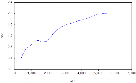
In case of China, the coefficient value of lnGDP is 1.50 which is positive and noteworthy and suggests that 1% addition in lnGDP will add to lnCO2 by 1.02% on average in the long run which proves the fact that the developing economies give more importance to economic growth as compared to environmental protection [63]. Whereas the coefficient value of lnGDP2 is -0.07 which suggests that 1% boost in lnGDP2 will cut per capita carbon emissions by 0.07% on average. These results prove that with a definite level of income is achieved any additional increase in income or economic growth will result in the improvement of environmental quality as environment protection becomes their primary objective. China is playing an active role in order to mitigate the environmental problems.
During last 10 years or so China has achieved a remarkable growth rate of 9.64% (Streets 2006). According to the ministry of Environmental protection (2004-2009) China has spent $240 billion USD over the period of 2003 to 2008 for protecting the environment which has led to decrease in soil erosion, improvement of wildlife habitats, increase in carbon sequestration, and increase in vegetation cover in some areas of the country [64-66]. Moreover, 1.49% of GDP was spent on environment in 2008. A decline of 6.61% and 8.95% in CO2 emissions and SO2 emissions was observed in 2008 as compared to that in 2005. Different environmental policies have been made after the year 2000 like government led standards & enforcements, pure markets, market based pure state whose primary objective is to attain economic growth while protecting the environment [16].
The outcomes of this paper are similar to [58, 67]. Furthermore, the landmark of GDP per capita estimated for China is $1071 USD. Figure 1 and Figure 2 show the graphical representation of the association among economic growth and CO2 discharges from 1970 to 2014. It is observed an inverted U shaped affiliation among two variables thus confirming the existence of EKC for China and India.
Moreover, the coefficient of domestic credit to private sector is positive as well as statistically significant for both countries. In China’s case, the coefficient value of 0.12% indicates that 1% increase in lnDCPS will enhance per capita carbon emissions by 0.12% on average in the long term. These results suggest that the loans provided by the banking sector to the enterprises or individuals are used in such projects and schemes that are damaging to the environment and result in air, land, and water pollution [68]. Sadorsky [39] explained that the loan provided by banking sector to households and private firms also results in the enhancement of CO2 emissions because the demand for good that require more energy increases like automobiles, air conditioners, and other household items while the private firms can invest in such businesses that are harmful for the environment. These results are also supported by [40, 44, 69].
Similarly, in case of India coefficient value of 0.26 is positive and significant suggests that 1% rise in lnDCPS will increase lnCO2 by 0.26% on average so we can conclude that credit provided to private sector has contributed towards CO2 discharges in long term. The results are consistent with [40].
Furthermore, the coefficient of energy use (lnEU) in case of China is 1.51 which is positive & significant. It suggests that 1% raise in lnEU will increase lnCO2 by 1.51% on average in the long term. According to Fang and Zeng (2007) coal, which is the major energy source in China, is responsible of producing 67% of nitrogen oxide (NO2), 90% of Sulphur dioxide (SO2) and 70% of the total Carbon CO2 in China. The coefficient of energy use is also positive & statistically significant in case of India which is an indication that energy use has a positive effect on the carbon emissions. The coefficient value of 2.90 suggests that 1% add to energy use will enhance carbon emissions by 2.90% on average in the long term. The results are consistent with [41, 58].
EKC (INDIA)
Figure 1. Relationship between Economic Growth and CO2 emissions (India)
EKC (CHINA)
Figure 2. Relationship between Economic Growth and CO2 emissions (China)
Additionally, in India’s case the coefficient of urbanization is positive and significant. This indicates that urbanization has resulted in higher carbon emissions. The coefficient value of 3.83 suggests that 1% escalation in urban population will escalate the per capita carbon emissions by 3.83% on average. According to Parikh and Shukla [42] urbanization increases direct & indirect demand of energy consumption which results in higher CO2emissions and environmental degradation. These results have support of [25]. However, the estimated model shows that coefficient of total population is positive but insignificant. China on the contrary, shows that the coefficient of urbanization is negative indicating that urbanization has not resulted in the increase of carbon emissions rather it has helped in controlling it in the long run while in the short term urbanization has found to have a positive impact on carbon discharges. The long term coefficient value of -2.07 suggests that 1% increase in urbanization will decrease CO2 discharge by 2.07% on average in the long term.
According to Poumanyvong and Kaneko [43] the sign of urbanizations coefficient depends upon the country’s developmental stage. If a country has high level of GDP per capita and the share of services sector is higher than manufacturing sector, then urbanization tends to improve the environmental conditions [70]. As the real per capita GDP of China grew at a rate of 8.16% over 1978 to 2004, structural transformation is also observed as the employment rate of agriculture sector has reduced from 69 to 33%. Our results are in line with [44]. However, positive and significant results are obtained for the coefficient of total population. The coefficient value of 1.26 explains that 1% boost in total population will enlarge CO2 discharges by 1.26% in the longer period of time. The results are in compliance with [43, 47].
The results of China show that the symbol of the ECM is negative and significant as desired for the co integration to exist. The value of -1.60 suggests that the previous year shocks that disturbed per capita CO2 emissions from its equilibrium value will be adjusted in the coming year. Similarly, the ECM term in case of India is -1.32 which is also negative and significant implying that the shocks that lead to the deviation of per capita carbon emissions from its equilibrium value will be adjusted inside the first year which means that the pace of shock regulation is really fast.
Figure 3. CUSUM and CUSUMSQ Test (India)
Figure 4. CUSUM and CUSUMSQ Test (China)
The last step in the ARDL is to check whether the model is stable or not. It is applied stability and diagnostic tests on our models. The results of serial correlation LM test is given in Table 5. Similarly, the plots show the results of the CUSUM and the square of Cumulative Sum Control Chart (CUSUMSQ) test for the model estimated for India and China. Figure 3 shows the plots for India which are within the critical bound values so we can conclude that the ECM variables are stable in this case. Similarly, Figure 4 shows the plot for China. The plots are within the critical bound values we conclude that every variable in the ECM is stable.
The primary aim of this study is to test whether EKC hypothesis holds or not with respect to India and Chin. Furthermore, the impact of population, financial development, urbanization and energy use on the per capita carbon emissions was also analyzed for both countries using STIRPAT framework. A time series analysis was done from 1980 to 2019. The results reveal that the EKC exists in case of India and China. The results are encouraging as it proves that economic growth is not as harmful as it could have been because it eventually results in the improvement of environmental quality. So no specific policy measures are required to be taken by the policy makers. Since, Nasir and Rehman [19] described that the EKC as an indicator specific phenomenon; the process of economic growth should be conducted in a carefully planned and cleverly organized manner.
On the contrary the results confirm that use of energy has a positive effect on CO2 discharges for both countries which is a serious issue and a point of concerns for policy makers. Strict laws must be enforced to replace the use of inefficient production methods and technologies which results in higher carbon emissions with environmental friendly technologies. For example, wind, solar, and hydrothermal sources should be used to generate electricity rather than coal. Similarly, environment friendly technologies in automobiles should be introduced in the market as cheaper and reliable substitute of the environmentally harmful technology.
Population has found to have a positive effect on the discharges for China but no significant impact was found in case of India. Increase in population increases the demand of electricity, buildings, automobiles, and food supply which are all energy driven causing an increase in the carbon emissions. Policies regarding population control need be executed until and unless it is switched towards environmental friendly processes. Moreover, the results show that financial development in India and China has resulted in environmental degradation. Sadorsky [39] explained that due to high household loans the demand of energy intensive goods like air conditioners, refrigerators, and vehicles are increasing which causes the per capita carbon emissions to increase. The policy makers are suggested to develop such policies so as to ensure provision of funds for the research and development on clean technologies in order to lowering the per capita carbon discharges.
Our findings further suggest that urbanization has caused increase of carbon discharges in case of India. So the policies regarding the process of urbanization should be made in a way that can affect the environment in the minimum possible manner by developing an eco-efficient urban infrastructure. Different projects such as plantation of trees especially in urban settlements must be initiated for the purpose of reduction in the CO2 emissions. Moreover, government should collaborate with the non-governmental organizations to create awareness among the people at national as well as regional level especially the new generation through advertisements, different campaigns, and social media about environmental protection. In case of China, results indicate that urbanization has not resulted in environmental degradation rather it has improved the environmental quality. Fang [70] explained that when a country achieves high per capita income and shifts towards a services based economy, growth of urbanization is not harmful for the environmental conditions which is true for China. Neither economic growth nor environmental conditions can be compromised, Ahmed and Long [71] maintained that our goal should be sustainable and environmental friendly economic development. We need to switch to eco-efficient process for protecting the environment but it will play an essential role in preserving the scarce natural resources and economic development through production efficiency.
[1] Fuglestvedt, J., Rogelj, J., Millar, R.J., Allen, M., Boucher, O., Cain, M., Forster, P.M., Kriegler, E., Shindell, D. (2018). Implications of possible interpretations of ‘greenhouse gas balance’ in the Paris Agreement. Philosophical Transactions of the Royal Society A: Mathematical, Physical and Engineering Sciences, 376(2119): 20160445. https://doi.org/10.1098/rsta.2016.0445
[2] Foster, G.L., Royer, D.L., Lunt, D.J. (2017). Future climate forcing potentially without precedent in the last 420 million years. Nature Communications, 8. http://www.cambridge.org/catalogue/catalogue.asp?isbn=9780521705967.
[3] Ozturk, I., Acaravci, A. (2010). CO2 emissions, energy consumption and economic growth in Turkey. Renewable and Sustainable Energy Reviews, 14(9): 3220-3225. https://doi.org/10.1016/j.rser.2010.07.005
[4] Ring, M.J., Lindner, D., Cross, E.F., Schlesinger, E.M. (2012). Causes of the global warming observed since the 19th century. Atmospheric and Climate Sciences, 2(4): 401-415. https://doi.org/10.4236/acs.2012.24035
[5] Dinda, S. (2004). Environmental Kuznets curve hypothesis: A survey. Ecological Economics, 49(4): 431-455. https://doi.org/10.1016/j.ecolecon.2004.02.011
[6] Kuznets, S. (2019). Economic growth and income inequality. The Gap Between Rich and Poor, 25-37. https://doi.org/10.4324/9780429311208-4
[7] Furuoka, F. (2015). Financial development and energy consumption: Evidence from a heterogeneous panel of Asian countries. Renewable and Sustainable Energy Reviews, 52: 430-444. https://doi.org/10.1016/j.rser.2015.07.120
[8] Tamazian, A., Bhaskara Rao, B. (2010). Do economic, financial and institutional developments matter for environmental degradation? Evidence from transitional economies. Energy Economics, 32(1): 137-145. https://doi.org/10.1016/j.eneco.2009.04.004
[9] Zhang, Y.J., Liu, Z., Zhang, H., Tan, T.D. (2014). The impact of economic growth, industrial structure and urbanization on carbon emission intensity in China. Natural Hazards, 73(2): 579-595. https://doi.org/10.1007/s11069-014-1091-x
[10] Frankel, J., Romer, D. (1999). Does trade cause growth? American Economic Review, 89(3): 379-299. https://doi.org/10.1257/aer.89.3.379
[11] Haseeb, A., Xia, E., Danish, Baloch, M.A., Abbas, K. (2018). Financial development, globalization, and CO2 emission in the presence of EKC: Evidence from BRICS countries. Environmental Science and Pollution Research, 25(31): 31283-31296. https://doi.org/10.1007/s11356-018-3034-7
[12] Zhang, J., Wang, L., Wang, S. (2012). Financial development and economic growth: Recent evidence from China. Journal of Comparative Economics, 40(3): 393-412. https://doi.org/10.1016/j.jce.2012.01.001
[13] Cohen, B. (2006). Urbanization in developing countries: Current trends, future projections, and key challenges for sustainability. Technology in Society, 28(1-2): 63-80. https://doi.org/10.1016/j.techsoc.2005.10.005
[14] Goldstone, J.A. (2002). Population and security: How demographic change can lead to violent conflict. Journal of International Affairs, 56(1): 3-21 https://doi.org/10.7551/mitpress/8210.003.0011
[15] Ali, H.S., Abdul-Rahim, A., Ribadu, M.B. (2016). Urbanization and carbon dioxide emissions in Singapore: evidence from the ARDL approach. Environmental Science and Pollution Research, 24(2): 1967-1974. https://doi.org/10.1007/s11356-016-7935-z
[16] Zhang, K., Wen, Z., Peng, L. (2007). Environmental policies in China: Evolvement, features and evaluation. China Population, Resources and Environment, 17(2): 1-7. https://doi.org/10.1016/s1872-583x(07)60006-0
[17] Zheng, G., Shi, S., Tang, H. (2005). Population development and the value of children in the People’s Republic of China. The Value of Children in Cross-Cultural Perspective: Case Studies from Eight Societies, 239-281. https://www.researchgate.net/profile/Bernhard-Nauck/publication/260369214_The_value_of_children_in_cross-cultural_perspective_Case_studies_in_eight_societies/links/56d6eb7308aee1aa5f75ad46/The-value-of-children-in-cross-cultural-perspective-Case-studies-in-eight-societies.pdf#page=235.
[18] Chaturvedi, V., Eom, J., Clarke, L.E., Shukla, P.R. (2014). Long term building energy demand for India: Disaggregating end use energy services in an integrated assessment modeling framework. Energy Policy, 64: 226-242. https://doi.org/10.1016/j.enpol.2012.11.021
[19] Nasir, M., Ur Rehman, F. (2011). Environmental Kuznets Curve for carbon emissions in Pakistan: An empirical investigation. Energy Policy, 39(3): 1857-1864. https://doi.org/10.1016/j.enpol.2011.01.025
[20] Grossman, G.M., Krueger, A.B. (1991) Environmental impacts of the North American free trade agreement. NBER, Working Paper 3914. https://doi.org/10.3386/w3914
[21] Panayotou, T. (1995). Environmental degradation at different stages of economic development. ILO Working Papers 992927783402676, International Labour Organization.
[22] Selden, T.M., Song, D. (1994). Environmental quality and development: Is there a Kuznets curve for air pollution emissions? Journal of Environmental Economics and Management, 27(2): 147-162. https://doi.org/10.1006/jeem.1994.1031
[23] Grossman, G., Krueger, A. (1995). Economic environment and the economic growth. Quarterly Journal of Economics, 110(2): 353-377 https://doi.org/10.2307/2118443
[24] Waslekar, S. (2012). Asia-Potential for Green Economy. University Grant Commission Sponsored, Ramnarain Ruia College.
[25] Kijima, M., Nishide, K., Ohyama, A. (2010). Economic models for the environmental Kuznets curve: A survey. Journal of Economic Dynamics and Control, 34(7): 1187-1201. https://doi.org/10.1016/j.jedc.2010.03.010
[26] Stern, D.I. (2004). The rise and fall of the environmental Kuznets curve. World Development, 32(8): 1419-1439. https://doi.org/10.1016/j.worlddev.2004.03.004
[27] Wang, Q.C. (2013) Analysis of the effects of population policy on carbon emissions in China. St. Decis., 13: 105-108. https://doi.org/10.3390/su10072458
[28] Alam, M.M., Murad, W., Noman, A.H.M., Ozturk, I. (2019). Relationships among Carbon Emissions, Economic Growth, Energy Consumption and Population Growth: Testing Environmental Kuznets Curve Hypothesis for Brazil, China, India and Indonesia, 70: 477-479. https://doi.org/10.31235/osf.io/8hq6z
[29] Pal, D., Mitra, S.K. (2017). The environmental Kuznets curve for carbon dioxide in India and China: Growth and pollution at crossroad. Journal of Policy Modeling, 39(2): 371-385. https://doi.org/10.1016/j.jpolmod.2017.03.005
[30] Kanjilal, K., Ghosh, S. (2013). Environmental Kuznet’s curve for India: Evidence from tests for cointegration with unknown structural breaks. Energy Policy, 56: 509-515. https://doi.org/10.1016/j.enpol.2013.01.015
[31] Boutabba, M.A. (2014). The impact of financial development, income, energy and trade on carbon emissions: Evidence from the Indian economy. Economic Modelling, 40: 33-41. https://doi.org/10.1016/j.econmod.2014.03.005
[32] Tamazian, A., Chousa, J.P., Vadlamannati, K.C. (2009). Does higher economic and financial development lead to environmental degradation: Evidence from BRIC countries. Energy Policy, 37(1): 246-253. https://doi.org/10.1016/j.enpol.2008.08.025
[33] Claessens, S., Feijen, E. (2007). Financial sector development and the millennium development goals. World Bank Working Papers. https://doi.org/10.1596/978-0-8213-6865-7
[34] Birdsall, N., Wheeler, D. (1993). Trade policy and industrial pollution in Latin America: Where are the pollution havens? The Journal of Environment & Development, 2(1): 137-149. https://doi.org/10.1177/107049659300200107
[35] King, R.G., Levine, R. (1993). Finance, entrepreneurship and growth. Journal of Monetary Economics, 32(3): 513-542. https://doi.org/10.1016/0304-3932(93)90028-e
[36] Shahbaz, M., Kumar Tiwari, A., Nasir, M. (2013). The effects of financial development, economic growth, coal consumption and trade openness on CO2 emissions in South Africa. Energy Policy, 61: 1452-1459. https://doi.org/10.1016/j.enpol.2013.07.006
[37] Jensen, V. (1996). The pollution haven hypothesis and the industrial flight hypothesis: some perspectives on theory and empirics. Centre for Development and the Environment, University of Oslo.
[38] Zhang, Y.J. (2011). The impact of financial development on carbon emissions: An empirical analysis in China. Energy Policy, 39(4): 2197-2203. https://doi.org/10.1016/j.enpol.2011.02.026
[39] Sadorsky, P. (2010). The impact of financial development on energy consumption in emerging economies. Energy Policy, 38(5): 2528-2535. https://doi.org/10.1016/j.enpol.2009.12.048
[40] Shahbaz, M., Loganathan, N., Muzaffar, A.T., Ahmed, K., Ali Jabran, M. (2016). How urbanization affects CO2 emissions in Malaysia? The application of STIRPAT model. Renewable and Sustainable Energy Reviews, 57: 83-93. https://doi.org/10.1016/j.rser.2015.12.096
[41] Jalil, A., Feridun, M. (2011). The impact of growth, energy and financial development on the environment in China: A cointegration analysis. Energy Economics, 33(2): 284-291. https://doi.org/10.1016/j.eneco.2010.10.003
[42] Parikh, J., Shukla, V. (1995). Urbanization, energy use and greenhouse effects in economic development. Global Environmental Change, 5(2): 87-103. https://doi.org/10.1016/0959-3780(95)00015-g
[43] Poumanyvong, P., Kaneko, S. (2010). Does urbanization lead to less energy use and lower CO2 emissions? A cross-country analysis. Ecological Economics, 70(2): 434-444. https://doi.org/10.1016/j.ecolecon.2010.09.029
[44] Zhang, N., Yu, K., Chen, Z. (2017). How does urbanization affect carbon dioxide emissions? A cross-country panel data analysis. Energy Policy, 107: 678-687. https://doi.org/10.1016/j.enpol.2017.03.072
[45] Al-mulali Usama, Weng-Wai, C., Sheau-Ting, L., Mohammed, A.H. (2015). Investigating the environmental Kuznets curve (EKC) hypothesis by utilizing the ecological footprint as an indicator of environmental degradation. Ecological Indicators, 48: 315-323. https://doi.org/10.1016/j.ecolind.2014.08.029
[46] Shahbaz, M., Shahzad, S.J.H., Ahmad, N., Alam, S. (2016). Financial development and environmental quality: The way forward. Energy Policy, 98: 353-364. https://doi.org/10.1016/j.enpol.2016.09.002
[47] He Z, Xu S, Shen W, Long R, Chen H (2017) Impact of urbanization on energy related CO2 emissions at different development levels: regional difference in china based on panel estimations. Journal of Cleaner Production, 140: 1719-1730. https://doi.org/10.1016/j.jclepro.2016.08.155
[48] Zarzoso, I., Maruotti, A. (2011). The impact of urbanization on CO2 emissions: Evidence from developing countries. Ecological Economics, 70(7): 1344-1353. https://doi.org/10.1016/j.ecolecon.2011.02.009
[49] Li, T., Wang, Y., Zhao, D. (2016). Environmental Kuznets Curve in China: New evidence from dynamic panel analysis. Energy Policy, 91: 138-147. https://doi.org/10.1016/j.enpol.2016.01.002
[50] Ehrlich, P.R., Holdren, J.P. (1971). Impact of population growth. Science, 171(3977): 1212-1217. https://doi.org/10.1126/science.171.3977.1212
[51] Dietz, T., Rosa, E.A. (1997). Effects of population and affluence on CO2 emissions. Proceedings of the National Academy of Sciences, 94(1): 175-179. https://doi.org/10.1073/pnas.94.1.175
[52] Dietz, T., Rosa, E.A. (1994). Rethinking the environmental impacts of population, affluence and technology. Human Ecology Review, 1(1994): 277-300. https://doi.org/10.1023/A:1017512325580
[53] York, R., Rosa, E.A., Dietz, T. (2003). STIRPAT, IPAT and impact: Analytic tools for unpacking the driving forces of environmental impacts. Ecological Economics, 46(3): 351-365. https://doi.org/10.1016/s0921-8009(03)00188-5
[54] Fu, B., Wu, M., Che, Y., Wang, M., Huang, Y.C., Bai, Y. (2005). The strategy of a low carbon economy based on the STIRPAT and SD models. Acta Ecological Sinica, 35(4): 76-82. https://doi.org/10.1016/j.chnaes.2015.06.008
[55] Diener, B.J., Frank, W.P. (2010). The China-India challenge: A comparison of causes and effects of global warming. International Business & Economics Research Journal (IBER), 9(3). https://doi.org/10.19030/iber.v9i3.533
[56] Phillips, P.C.B. (1986). Understanding spurious regressions in econometrics. Journal of Econometrics, 33(3): 311-340. https://doi.org/10.1016/0304-4076(86)90001-1
[57] Granger, C.W.J., Newbold, P. (1974). Spurious regression in Econometrics. Journal of Econometrics, 2(2): 111-120. https://doi.org/10.1016/0304-4076(74)90034-7
[58] Jalil, A., Mahmud, S.F. (2009). Environment Kuznets curve for CO2 emissions: A cointegration analysis for China. Energy Policy, 37(12): 5167-5172. https://doi.org/10.1016/j.enpol.2009.07.044
[59] Pesaran, M.H., Pesaran, B. (1997). Working with Microfit 4.0: Interactive Econometric Analysis. Oxford University Press, Oxford.
[60] Pesaran, M.H., Shin, Y. (1999). An autoregressive distributed-lag modelling approach to cointegration analysis. Econometrics and Economic Theory in the 20th Century, pp. 371-413. https://doi.org/10.1017/cbo9781139052221.011
[61] Pesaran, M.H., Shin, Y., Smith, R.J. (2001). Bounds testing approaches to the analysis of level relationships. Journal of Applied Econometrics, 16(3): 289-326. https://doi.org/10.1002/jae.616
[62] Jayanthakumaran, K., Verma, R., Liu, Y. (2012). CO2 emissions, energy consumption, trade and income: A comparative analysis of China and India. Energy Policy, 42: 450-460. https://doi.org/10.1016/j.enpol.2011.12.010
[63] Beckerman, W. (1992). Economic growth and the environment: Whose growth? whose environment? World Development, 20(4): 481-496. https://doi.org/10.1016/0305-750x(92)90038-w
[64] Cao, S. (2008). Why large-scale afforestation efforts in china have failed to solve the desertification problem. Environmental Science & Technology, 42(6): 1826-1831. https://doi.org/10.1021/es0870597
[65] Piao, S., Fang, J., Ciais, P., Peylin, P., Huang, Y., Sitch, S., Wang, T. (2009). The carbon balance of terrestrial ecosystems in China. Nature, 458(7241): 1009-1013. https://doi.org/10.1038/nature07944
[66] Liu, J. (2008) Ecological and socioeconomic effects of China’s policies for ecosystem services. Proc Natl Acad Sci USA, 105(28): 9477-9482 https://doi.org/10.1073/pnas.0706436105
[67] Song, T., Zheng, T., Tong, L. (2008). An empirical test of the environmental Kuznets curve in China: A panel cointegration approach. China Economic Review, 19(3): 381-392. https://doi.org/10.1016/j.chieco.2007.10.001
[68] Wang, C.M., Lin, Z.L. (2010). Environmental policies in china over the past 10 years: Progress, problems and prospects. Procedia Environmental Sciences, 2: 1701-1712. https://doi.org/10.1016/j.proenv.2010.10.181
[69] Javid, M., Sharif, F. (2016). Environmental Kuznets curve and financial development in Pakistan. Renewable and Sustainable Energy Reviews, 54: 406-414. https://doi.org/10.1016/j.rser.2015.10.019
[70] Fang, Y., Zeng, Y. (2007). Balancing energy and environment: The effect and perspective of management instruments in China. Energy, 32(12): 2247-2261. https://doi.org/10.1016/j.energy.2007.07.016
[71] Ahmed, K., Long, W. (2012). Environmental Kuznets curve and Pakistan: An empirical analysis. Procedia Economics and Finance, 1: 4-13. https://doi.org/10.1016/s2212-5671(12)00003-2