Gerusa C. Rodrigues | Giulio Lorenzini* | Lucas C. Victoria | Igor S. Vaz | Luiz A.O. Rocha | Elizaldo D. dos Santos | Michel K. Rodrigues | Emanuel da S. D. Estrada | Liércio A. Isoldi
© 2021 IIETA. This article is published by IIETA and is licensed under the CC BY 4.0 license (http://creativecommons.org/licenses/by/4.0/).
OPEN ACCESS
An Earth-Air Heat Exchanger (EAHE) is a device that consists of one or more buried ducts through which air is forced to flow. The surrounding soil is responsible for enabling thermal exchanges along with the installation, making the temperature at the outlet milder than the inlet. The objective of this work is to ally a numerical-analytical approach with the Constructal Design method and Exhaustive Search technique to minimize the soil volume occupation (V), minimize the air flow pressure drop (PD), and maximize the thermal potential (TP) of a T-shaped EAHE. Starting from a conventional EAHE composed of a straight duct, called Reference Installation (RI), two degrees of freedom (DOF) were considered: the ratio between the length of the bifurcated branch and the length of the main branch (L1/L0) and the ratio between the diameter of the bifurcated branch and the diameter of the main branch (D1/D0). Comparing with RI, different T-shaped EAHE geometries were identified to reduce V by 23% and PD by 62% and to increase TP by 21%; and when these three performance parameters were concomitantly considered another T-shaped EAHE geometric configuration allowed to reach an improvement of around 27% when compared with the RI.
constructal design, computational fluid dynamics (CFD), earth-air heat exchanger (EAHE), finite volume method (FVM), numerical simulation, thermal comfort
Energy consumption is an important factor to be taken into account in engineering projects. Regarding the Civil Construction industry, one of the main concerns of the market players is to develop products with low electrical energy usage to provide comfort to its users. Studies show that 10% of global energy expenditure results from traditional air conditioning systems, cooling, or heating devices [1], and it can reach levels of 20 to 40 % in developed countries [2, 3].
In Brazil, it is possible to notice the rise in electricity consumption due to air conditioners within the last years. A local company was able to estimate this growth as being three times the levels of consumption of 2006 due to the expanding rate of these equipment sales, taken a 9% increase each year for the period of 2005 to 2017 [4].
As a consequence of this demand, the development of technologies to reach acceptable comfort levels with less electricity consumption has increasingly become a focus of various studies. Another course of action for solving this problem is investigating ways to use renewable energies instead of an electrical one. It is known that the radiation emitted by the Sun is the main source of clean energy [5] and, in Vaz et al. [6, 7], one can note that the soil can be used as a reservoir of thermal energy with the adoption of Earth-Air Heat Exchangers (EAHE) to reduce the usage of traditional air conditioning systems. These devices are relatively simple to build and install, mainly in new buildings, since their materials can be easily found on the market and no specialized workforce is needed to put them into service. In addition to this, its operating principle is also simple: the air is forced to flow into buried ducts exchanging heat with the surrounding soil, resulting in a milder air temperature at the EAHE outlet when compared to its inlet temperature.
Many studies were carried out aiming to investigate the EAHE thermo-fluid-dynamic behavior using different approaches, such as experimental [7-10], analytical [11-13], and numerical [14-18]. Since experimental research is time-consuming and financially onerous, in reason of the period needed to be monitored to achieve a good level of knowledge of its behavior – taken as one entire year to embrace all seasons, other approaches appear as the best way to fulfill this necessity of studies. Hence, the numerical method, usually solved with the help of computers, is the faster way to develop new research concerning its geometry optimization and operational parametric analysis.
Regarding the numerical researches, two main streams can be identified in the literature. On one side, it stands up for the implementation of one-dimensional analytical studies, such as given by Papakostas et al. [19], Benkert et al. [20], and De Paepe and Janssens [21]. This methodology is considered adequate for a preliminary project and designing aspects since it is quickly solved and generates satisfactory results. However, it is only appropriate for simpler installations, such as straight duct buried on non-stratified soil. For more complex geometric configurations and soil stratifications, the two and three-dimensional models are usually adopted, being this the other stream of studies. In this particular type of work, the full soil thermo-physical properties, such as density, specific heat, and thermal conductivity, are taken into account, and the air flow inside ducts are considered unsteady, turbulent, and incompressible, in contrast to the laminar modeling adopted by some 1-D studies.
Vaz et al. [6, 7] carried out a pioneer experimental study for an EAHE installed in the city of Viamão, in the south of Brazil. It was developed a complex geometry with multiple ducts, and the air and soil temperatures were monitored every 30 min throughout the year 2007. The study also included experiments in determining the thermo-physical properties of the soil and the air, aiming to reproduce computationally the thermo-fluid-dynamic behavior observed in loco. Since that, other works took place to improve the computational model developed in Vaz et al. [6], like in Brum et al. [15], where it was validated using a reduced model, making it possible to simulate the EAHE operation with less computational effort. After that, in Rodrigues et al. [16], it was proposed to enhance this model with the employment of a simpler turbulence model, allowing a reduction in processing time with no accuracy loss.
Another widely used approach for the analysis of Heat Transfer systems consists in the application of the Constructal Design method in association with the computational modeling, as in Adewumi et al. [22] and Gulotta et al. [23]; being this approach also used for the study of EAHE, as in Rodrigues et al. [16] and Brum et al. [24].
The Constructal Design is based on the Constructal Law theory developed by Bejan [25], which states that "for a finite-size flow system to persist in time (to live) it must evolve such that it provides greater and greater access to the currents that flow through it."
In this context, the present article aims to study a T-shaped EAHE for the city of Viamão, in the central region of the state of Rio Grande do Sul, in southern Brazil. The Constructal Design was applied to propose different EAHE T-shaped geometries that can be properly compared to each other. In other words, the Constructal Design was adopted to define the search space. In sequence, the thermal behavior of each EAHE configuration was numerically simulated, while its soil volume occupation and air flow pressure drop were analytically determined. Then, using the Exhaustive Search technique, it was possible to identify the best T-shaped EAHE geometric configurations that maximize the thermal potential (TP), minimize the soil volume occupation (V), and minimize the air flow pressure drop (PD). Finally, considering these three performance parameters concomitantly and performing a vector analysis, it was possible to indicate the optimized geometry for the T-shaped EAHE.
It is important to highlight that the contribution of the present work if compared with other studies, as [6, 7, 15, 16, 24], relies on the analysis of the T-shaped geometry for an EAHE (having one inlet and two outlets); allowing to investigate the influence of two degrees of freedom (DOF) over the EAHE performance: The ratio between the length of the bifurcated branches and the length of the main branch (L1/L0); and the ratio between the diameter of the bifurcated branches and the diameter of the main branch (D1/D0).
The Constructal Design application starts based on an EAHE adopted as a reference and composed of a straight duct 30 m long and 110 mm in diameter, having one inlet and one outlet for the air flow. This case, called Reference Installation (RI), is depicted in Figure 1, being buried at a depth of 3 m on a 15 m high portion of the soil, as recommended in Brum et al. [15].
From RI, the T-shaped EAHE geometric configurations were defined, having the aspect indicated in Figure 2.
Figure 1. Reference Installation (RI)
Figure 2. T-shaped EAHE: (a) perspective; and (b) superior view
The T-shaped geometries were generated respecting the following constraints (see Figure 2b): The total duct length (LTotal) given by:
$L_{T o t a l}=L_{R I}=L_{0}+2 L_{1}=30 \mathrm{~m}$ (1)
where, LRI is the length of the RI duct (in m, see Figure 1), L0 is the length of the main branch (m), and L1 is the length of the bifurcated branch (m); so the total duct volume (VDuct) is defined as:
$V_{\text {Duct }}=\frac{\pi}{4} L_{R I} D_{R I}^{2}=\frac{\pi}{4} L_{0} D_{0}^{2}+\frac{\pi}{4} L_{1} D_{1}^{2}=0.285 \mathrm{~m}^{3}$ (2)
being DRI the RI diameter (in m, see Figure 1), D0 the diameter of the main branch (m), and D1 the diameter of the bifurcated branch (m). As in RI (see Figure 1), for the T-shaped geometries, the installation depth is h = 3 m, and the soil portion height is H = 15 m (see Figure 2a).
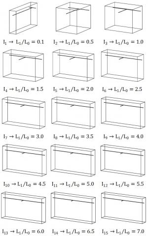
In addition to these constraints, the two degrees of freedom (DOF) were varied. The first DOF was the ratio L1/L0, varying in a range from 0.1 to 7.0 and generating the installation I1 to I15, as illustrated in Figure 3.
Figure 3. T-shaped EAHE obtained due to the L1/L0 variation
The ducts length for the main and bifurcated branches of the EAHEs depicted in Figure 3 are in Table A of the Appendix.
The second varied DOF was the ratio D1/D0. Initially, its value was assumed to be equal to 1.00, being D1 = D0 = 110 mm (i.e., the same diameter of RI). Thereafter, variations in this DOF were stipulated, considering contractions when D0 > D1 (D1/D0 = 0.50 and D1/D0 = 0.75 - see Table B of Appendix) and expansions when D0 < D1 (D1/D0 = 1.25 and D1/D0 = 1.50 - see Table C of Appendix).
Therefore, considering the variations of the ratios L1/L0 and D1/D0, a total of 75 T-shaped EAHE installations were proposed to form the search space of this analysis.
In sequence, the RI and the 75 T-shaped installations were analyzed. To do so, the thermal behavior of these EAHE was numerically simulated through a computational model in the Fluent software, which is based on the Finite Volume Method (FVM), allowing to define the thermal potential (TP) of each installation. In its turn, the soil volume (V) occupied for each installation and its air pressure drop (PD) were analytically defined.
2.1 Numerical approach
The employed computational model was previously verified and validated by Brum et al. [15] and Rodrigues et al. [16] by means the numerical and experimental results of Vaz et al. [6, 7]. So, for brevity, the computational model verification and validation were not presented here in detail.
It is important to mention that regardless of the L1/L0 and D1/D0 values, the distance d between the ducts and the domain wall (see Figure 2b) was equal to 2 m. The reason behind it is to avoid jeopardized results due to boundary conditions set in these walls [16].
From this, and considering the Constructal Design method application, the geometry of the computational domains of the RI (see Figure 1) and the T-shaped EAHEs (see Figures 2 and 3) were defined. The spatial discretization of these computational domains was generated according to Rodrigues et al. [16], being the mesh composed of tetrahedral computational cells with a size equivalent to 3D for the soil, while in the duct the size of computational cells was D/3. Remembering that D is the EAHE duct diameter which due to the variation of the DOF D1/D0 can assume different values, but always being the smallest diameter adopted to promote the domain discretization. Moreover, to avoid mesh generation issues, the ducts' thickness and material properties were disregarded. Consequently, the air is considered to pass through the boreholes in the soil portion, being this simplification widely adopted in EAHE numerical simulations, as in Vaz et al. [6], Brum et al. [15, 24], and Rodrigues et al. [16].
The numerical simulations were performed by solving the energy equation for the soil [26]:
$\frac{\partial T}{\partial t}=\frac{\partial}{\partial x_{j}}\left(\alpha_{s} \frac{\partial T}{\partial x_{j}}\right)$ (3)
where, T is the soil temperature field (K), t is the time (s), $x_{j}$ represents the spatial coordinates (m), as is the soil thermal diffusivity (m²/s), and j = 1, 2, and 3; in addition to the conservation equations of mass, momentum, and energy for the transient, incompressible, and turbulent forced convective air flow inside the EAHE duct, respectively, given by [26, 27]:
$\frac{\partial \overline{v_{i}}}{\partial x_{i}}=0$ (4)
$\frac{\partial \overline{v_{i}}}{\partial t}+\frac{\partial\left(\overline{v_{i} v_{j}}\right)}{\partial x_{j}}=-\frac{1}{\bar{\rho}} \frac{\partial \bar{p}}{\partial x_{j}} \delta_{i j}+\frac{\partial}{\partial x_{j}}\left[v\left(\frac{\partial \overline{v_{i}}}{\partial x_{j}}+\frac{\partial \overline{v_{j}}}{\partial x_{i}}\right)-\tau_{i j}\right]$ (5)
$\frac{\partial \bar{T}}{\partial t}+\frac{\partial}{\partial x_{j}}\left(\overline{v_{j} T}\right)=\frac{\partial}{\partial x_{j}}\left(\alpha \frac{\partial \bar{T}}{\partial x_{j}}-q_{j}\right)$ (6)
where, the over line represents the time-averaged terms, xi are the spatial coordinates (m), vi are the velocity in Cartesian directions (m/s), dij is the Kronecker delta, p is the pressure (Pa), u is the air kinematic viscosity (m²/s), a is the air thermal diffusivity (m²/s), and i, j = 1, 2, 3. The terms tij and qj that arise in the filtering process of the momentum and energy conservation equation, respectively, need to be modeled and can be written as [28]:
$\tau_{i j}=\overline{v_{i}^{\prime}} \overline{v_{j}^{\prime}}$ (7)
$q_{j}=\overline{v_{i}^{\prime}} \overline{T^{\prime}}$ (8)
where, the (') indicates the time varying fluctuating component.
To deal with the closure problem, the RANS k-ε model is employed, which is based on the solution of two additional transport equations. For incompressible flows, the closure terms of Eqns. (7) and (8) are given by [28]:
$\tau_{i j}=v_{t}\left(\frac{\partial \bar{v}_{i}}{\partial x_{j}}+\frac{\partial \bar{v}_{j}}{\partial x_{i}}\right)-\frac{2}{3} k \delta_{i j}$ (9)
$q_{j}=\alpha_{t} \frac{\partial \bar{T}}{\partial x_{j}}$ (10)
where, ut is the kinematic eddy viscosity (m2/s), k is the turbulent kinetic energy (m2/s2) and at is the thermal eddy diffusivity (m2/s). The values of ut and at can be defined as:
$v_{t}=C_{\mu} \frac{k^{2}}{\varepsilon}$ (11)
$\alpha_{t}=\frac{v_{t}}{\operatorname{Pr}_{t}}$ (12)
where, Cμ = 0.09 and Prt = 1.00. The turbulent kinetic energy (k) and turbulent dissipation (ε) are, respectively [28]:
$\frac{\partial k}{\partial t}+\bar{v}_{j} \frac{\partial k}{\partial x_{j}}=\tau_{i j} \frac{\partial \bar{v}_{i}}{\partial x_{j}}+\frac{\partial}{\partial x_{j}}\left[\left(v+\frac{v_{t}}{\sigma_{k}}\right) \frac{\partial k}{\partial x_{j}}\right]-\varepsilon$ (13)
$\frac{\partial \varepsilon}{\partial t}+\bar{v}_{j} \frac{\partial \varepsilon}{\partial x_{j}}=\frac{\partial}{\partial x_{j}}\left[\left(v+\frac{v_{t}}{\sigma_{\varepsilon}}\right) \frac{\partial \varepsilon}{\partial x_{j}}\right]+C_{\varepsilon 1} \frac{\varepsilon}{k} \tau_{i j} \frac{\partial \bar{v}_{i}}{\partial x_{j}}-C_{\varepsilon 2} \frac{\varepsilon^{2}}{k}$ (14)
being Cε1 = 1.44 and Cε2 = 1.92.
In the current study, the mathematical model was numerically solved through the FVM with the aid of the Fluent software, where a transient and pressure-based solution was performed. The first-order upwind scheme was set to deal with the arising instabilities of the advective terms. In relation to the pressure-velocity coupling, the SIMPLE algorithm was used. Concerning the convergence criteria, the residues for the mass, momentum, and energy were considered converged when the residues between two consecutive iterations are lower than 1×10⁻³, 1×10⁻³, and 1×10⁻⁶, respectively. The processing time was equivalent to two simulated years for all the simulations, totaling 17520 time steps of 3600 s (1 h) each. However, the first simulated year is neglected to avoid interference of the initial conditions in the results.
As in Vaz et al. [6] and Brum et al. [15], for each numerical simulation, the initial temperature condition of the entire domain is assumed equal to the average soil temperature of 291.70 K (18.70℃).
Regarding the boundary conditions, also based on Vaz et al. [6] and Brum et al. [15], the inlet air prescribed velocity is 3.3 m/s; and the prescribed annual temperature variation at the air inlet, Tin(t), and at the superior soil surface, Tss(t), are, respectively, given by:
$T_{i n}(t)=296.18+6.92 \cdot \sin \left(200 \times 10^{-9} \cdot t+26.42\right)$ (15)
$T_{s s}(t)=291.70+6.28 \cdot \sin \left(200 \times 10^{-9} \cdot t+26.24\right)$ (16)
The transient functions presented in Eqns. (15) and (16) were generated from the adjustment of the experimental data monitored during 2007 in the city of Viamão [7]. The other soil surfaces of the computational domain were considered thermally insulated (qʺ = 0 W/m²), while a manometric pressure was assumed at the EAHE outlets (pout = 0 Pa) and non-slip and impermeability conditions were imposed at the duct walls.
Moreover, the soil and air thermo-physical properties were considered the same way as in Vaz et al. [7]. The geotechnical profile of Viamão soil is homogeneous and with clayey characteristics, being its density (r), thermal conductivity (l), and specific heat (cp) assumed as isotropic and constant [29]. Concerning the air, these properties, together with its absolute viscosity (m), were assumed as constants in agreement with Brum et al. [15] and Lee et al. [30]. The values of the thermo-physical properties for the soil and the air are presented in Table 1.
Table 1. Thermo-physical properties for the air and the soil
|
Material |
r (kg/m3) |
l (W/m·K) |
cp (J/kg·K) |
m (kg/m·s) |
|
Soil |
1,800 |
2.1 |
1,780 |
- |
|
Air |
1.16 |
0.0242 |
1,010 |
1.798×10⁻⁵ |
2.2 Performance parameters
As previously stated, three different performance parameters were evaluated for this study: the occupied soil volume (V), the air pressure drop (PD), and the EAHE thermal potential (PT). The performance parameters were normalized through the Reference Installation (RI) results to perform a geometric optimization using the Exhaustive Search technique to the T-shaped EAHE geometric configurations proposed by the Constructal Design method.
Therefore, the normalized soil volume occupied by the T-shaped EAHEs is obtained as:
$V_{N}=\frac{V_{T}}{V_{R I}}=\frac{W \cdot L \cdot H}{V_{R I}}$ (17)
being VT, W, L, and H, respectively, the volume, width, length, and high of the T-shaped soil portion (see Figure 2b), and VRI = 2,250 m3 is the RI soil volume (see Figure 1). Wherefore, as H is kept constant and equal to 15 m, VT depends directly on the L1/L0 value, since this ratio changes the values of L and W of the soil portion.
In its turn, the pressure drop (PD) in the forced turbulent air flow inside the EAHE duct comprises distributed losses in its straight stretches (PDd) and localized losses related to the flow discontinuities (PDl), being defined as [31]:
$P D=\sum P D_{d}+\sum P D_{l}$ (18)
where:
$P D_{d}=f \cdot \frac{L_{d}}{D} \cdot \frac{v^{2}}{2 g}$ (19)
and
$P D_{l}=K_{l} \cdot \frac{v^{2}}{2 g}$ (20)
being ƒ the friction factor; Ld the length of the straight duct (m); v the air velocity (m/s); D the duct diameter (m); g the gravitational acceleration (9.81 m/s2); and Kl the localized loss coefficient. It is possible to obtain the friction factor f with a correlation developed by Petukhov [32]:
$f=\left(0.79 \ln \operatorname{Re}_{D}-1.64\right)^{2}$ (21)
where, ReD is the air flow Reynolds number, given by [27]:
$\operatorname{Re}_{D}=\frac{\rho \cdot v \cdot D}{\mu}$ (22)
Concerning Eq. (20), for the T-shaped EAHEs, the T-joint was considered having a Kl = 1.8; while the contractions or expansions due to the D1/D0 variations were defined as indicated in [31] for the loss coefficients for flow through sudden area changes, being Kl = 0.40; 0.16; 0.12; and 0.30, respectively, for D1/D0 = 0.50; 0.75; 1.25; and 1.50.
From this, the normalized pressure drop (PDN) for the T-shaped EAHE installations was obtained as:
$P D_{N}=\frac{P D_{T}}{P D_{R I}}$ (23)
where, PDT is the pressure drop of the T-shaped EAHE and PDRI = 3.81 m is the pressure drop of the RI.
Finally, the Thermal Potential (TP) was adopted to the thermal performance of the EAHEs, being determined from an annual averaged air temperature. The TP of the EAHE installation can be expressed by [15, 16]:
$T P=\sqrt{\frac{\sum_{i=1}^{1460}\left(T(t)_{i}^{o u t}-T(t)_{i}^{i n}\right)^{2}}{1460}}$ (24)
where, T(t)out is the transient air temperature (in K or ℃) at the duct outlet; T(t)in is the transient air temperature (in K or ℃) at the duct inlet (prescribed temperature condition), and i varies from 1 to 1460 representing the outlet temperature measurements performed every 21,600 s during the second year of the numerical simulation. Thereby, the normalized TP (TPN) is given by:
$T P_{N}=\frac{T P_{T}}{T P_{R I}}$ (25)
being TPTthe thermal potential of the T-shaped EAHE and TPRI = 3.35℃ the thermal potential of the RI.
It is important to highlight that to reach the superior EAHE performance, while VN and PDN should be minimized, TPN must be maximized. When these parameters are analyzed individually, there is no problem; however, for a global analysis taking into account concomitantly the three performance parameters, it was necessary to consider the minimization of $T P_{N}^{-1}$ Therefore, for the global evaluation it was adopted a vector approach, given by:
$\mid$ Performance $\mid=\sqrt{\left(V N_{N}\right)^{2}+\left(P D_{N}\right)^{2}+\left(T P_{N}^{-1}\right)^{2}}$ (26)
From Eq. (26), an ideal hypothetical EAHE would have a null value for the $\mid$ Performance $\mid$ achieved with a VN = 0, PDN = 0, and $T P_{N}^{-1}=0$. Hence, the T-shaped EAHE having the lowest value of $\mid$ Performance$\mid$ will be the one with the best overall performance.
2.3 Geometric optimization
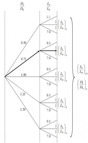
Figure 4. Constructal design associated with Exhaustive Search procedure
As earlier mentioned, the Constructal Design application allows defining the geometric configurations of the T-shaped EAHE, forming the search space. In addition to that, these cases were compared among each other, promoting a geometric optimization using the Exhaustive Search technique.
Figure 4 illustrates the steps of the optimization procedure. For each of the five values of D1/D0, fifteen values for the ratio L1/L0 were adopted (see Figure 3). From this, it was possible to identify the optimal value of L1/L0, (L1/L0)o, being the once optimized geometric configuration that leads to the superior performance of the T-shaped EAHE. After that, it was defined the twice optimized L1/L0, (L1/L0)2o, and the once optimized D1/D0, (D1/D0)o, reaching the superior performance among all cases of the search space.
This optimization procedure was employed for each performance parameter, i.e., by means Eqns. (17), (23), and (25); as well as concomitantly for the tree performance parameters through Eq. (26).
As previously indicated, a Reference Installation (RI) was adopted to normalize the T-shaped EAHEs performance. The thermal behavior of RI was presented in Fig. 5, showing the consistency of the numerical results generated with the computational model.
From Figure 5, the annual air variation of the RI outlet air is in perfect agreement with the results of Brum et al. [15] and Rodrigues et al. [16]. Since the computational model was verified and validated in these references, it is possible to prove the coherence of the numerical results generated in the present work. One can note in Figure 5 that the EAHE RI can provide milder temperatures almost every year. It can reach up to approximately -8℃ during the summer (months of January and December) and around +2℃ during the winter (months of June and July).
Besides, the annual averaged thermal potential for the RI was TPRI = 3.35℃, while the soil volume occupation and the pressure drop for The RI were, respectively, VRI = 2,250 m3 and PDRI = 3.81 m. Hence, these values were used as a normalizing factor in the T-shaped EAHE cases.
So, with the Constructal Design and Exhaustive Search association (see Figure 4), it is possible to perform a geometric evaluation and a geometric optimization, i.e., in addition to defining the optimized geometry that leads to the superior performance of the T-shaped EAHE, it was also possible to evaluate the influence of the degrees of freedom over the performance parameters.
Taking that into account, the results obtained individually and concomitantly for the three performance parameters are presented in sequence.
3.1 Occupied soil volume
From Eq. (17), the normalized soil volume occupied for each T-shaped EAHE of Figure 3 was defined and shown in Figure 6 for the five values of D1/D0.
Figure 6 shows the influence of the ratio L1/L0 between the length of the main and bifurcated branches on the normalized soil volume occupation, with the curves for the different values of D1/D0 practically superimposed. This no relevant influence of the D1/D0 DOF was already expected because the soil portion does not suffer significant change due to D1/D0 variation. On the other hand, regarding the L1/L0 DOF effect, one can assume that the minimization of the occupied soil occurs when L1 >> L0, since in all studied cases resulted in installation 15 as the best option. Therefore, the best ratio for soil occupation parameter was taken as (L1/L0)o = 7.0, reaching reductions around 23 % and 94 % if compared with RI and the worst T-shaped geometry (with L1/L0 = 0.5), respectively.
Despite the small influence of the D1/D0, following the optimization procedure (see Figure 4), Figure 7 presents the values of (L1/L0)o as a function of the D1/D0 variation.
As earlier observed, the effect of D1/D0 is no significant. A reduction of less than 0.4 % is achieved between the twice optimized configuration, with (L1/L0)2o = 7.0 and (D1/D0)o = 0.50, and the worst geometry of Fig. 7, with (L1/L0)o = 7.0 and D1/D0 = 1.50.
Figure 5. Annual air temperature variation for the RI
Figure 6. Influence of L1/L0 over VN, for each D1/D0
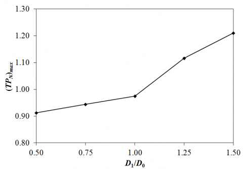
Figure 7. Influence of D1/D0 over (VN)min, from (L1/L0)o values
In summary, it is possible to reach out that the minimum soil occupation was achieved by the installation (L1/L0)oo = 7.0 and (D1/D0)o = 0.50, with a twice minimized volume of (VN)2min = 0.765 (representing a soil volume of 1,721.25 m3).
3.2 Pressure drop
Regarding the pressure drop imposed on the EAHE air flow, it was analytically calculated in its normalized version, according to Eq. (23). The effect of the ratio L1/L0 over the normalized pressure drop (PDN) is presented in Figure 8 for the five ratios of D1/D0.
One can infer in Figure 8 that the L1/L0 DOF has a low influence over the pressure drop, being the main difference a consequence of the D1/D0 DOF. However, it is possible to highlight L1/L0 = 7.0 as the once optimized geometric configuration to minimize the pressure drop among these configurations. If compared the performances of the best and worst T-shaped EAHE geometries for each D1/D0, improvements of 14.90 %, 19.25 %, 58.16 %, 67.66 %, and 66.67 % were, respectively, achieved. Moreover, in a general way, only the cases with D1/D0 ≥ 1.00 and L1/L0 ≥ 1.0 lead to a reduction in pressure drop compared to RI.
Figure 8. Influence of L1/L0 over PDN, for each D1/D0
Figure 9. Influence of D1/D0 over (PDN)min, from (L1/L0)o values
Another aspect indicated by Figure 8 is that from D1/D0 = 1.00 and L1/L0 = 2.0 is possible to observe a practically linear behavior for the pressure drop; while for D1/D0 values less than 1.00 fluctuations occur in the pressure drop magnitude due to the L1/L0 variation.
In sequence, the optimized values of L1/L0 that conduct to the once minimized PDN (identified in Figure 8) were plotted as a function of D1/D0 ratio in Figure 9.
The results of Figure 9 indicate that for D1/D0 = 1.00, 1.25, and 1.50, the values of (PDN)min are similar, being 0.47, 0.38, and 0.44, respectively, allowing a decrease of pressure drop in relation to RI; whereas for D1/D0 = 0.50 and 0.75, a pressure drop augmentation occurred. From this, the optimized T-shaped EAHE considering the both DOF is defined by (L1/L0)oo = 7.0 and (D1/D0)o = 1.25, which reaches a (PDN)2min = 0.38 (representing a pressure drop of 1.45 m) being a performance 62% superior to RI.
3.3 Thermal potential
The thermal potential is taken as the difference between the air temperature at the outlet and the inlet of the EAHE, measuring its capability to provide or remove heat from the air flow. So, as defined by Eq. (25), Figure 10 presents the normalized thermal potential of the T-shaped EAHEs according to the L1/L0 variation for all studied D1/D0.
Analyzing Figure 10 and remembering that the thermal potential should be maximized, it is possible to infer that the superior performances for the T-shaped EAHEs were achieved for small values of L1/L0. When D1/D0 = 0.50, 0.75, and 1.00, (L1/L0)o = 0.1; and when D1/D0 = 1.25 and 1.50, (L1/L0)o = 0.5. Besides, in a general way, the effect of L1/L0 variation over TPN is more pronounced as D1/D0 decreases. This fact is proved if the best and worst geometries for D1/D0 = 0.50 and D1/D0 = 1.50 are compared. In the last situation a difference of around only 15% occurs, while in the first one a difference of almost 50% is reached.
After the first stage of the optimization procedure (see Figure 4) regarding the thermal potential performance, the influence of D1/D0 DOF over the (L1/L0)o was evaluated in Figure 11.
Figure 10. Influence of L1/L0 over TPN, for each D1/D0
Figure 11. Influence of D1/D0 over (TPN)min, from (L1/L0)o values
One can note in Figure 11, as well as in Figure 10, that only the geometries with D1/D0 = 1.25 and 1.50 reached superior performances than the RI. The T-shaped EAHE geometry with (L1/L0)oo = 0.5 and (D1/D0)o = 1.50 achieves a (TPN)2max = 1.21 (representing a thermal potential of 4.05℃), being 21% better than the RI.
3.4 Global performance
Finally, the three performance parameters already individually analyzed were concomitantly taken into account. The goal here was to identify the optimized T-shaped EAHE that at the same time reduces the soil volume and pressure drop and increases the thermal potential. Eq. (26) was employed to the 75 T-shaped EAHE, and its results can be viewed in Figure 12 as a function of L1/L0 variation.
The results of Figure 12 indicate that the best geometric configuration was always obtained with L1/L0 = 7.0, regardless of the value of D1/D0.
Besides, one can observe in Fig. 12 that the T-shaped EAHE installations with D1/D0 = 0.75 and mainly D1/D0 = 0.50 presented inferior performances, since the smallest values in the vector analysis indicate the superior global performance. This result was already expected, once these cases have the worst performance regarding the pressure drop (see Figure 8) and thermal potential (see Figure 10) evaluations. Because of that, these geometries were removed from Figure 12, allowing in Figure 13 a better visualization. In addition, the result of Eq. (26) to the RI was also included in Figure 13, making possible a more comprehensive discussion.
Figure 12. Influence of L1/L0 in the vector analysis, for each D1/D0
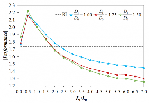
Figure 13. Influence of L1/L0 in the vector analysis, for the RI and the T-shaped EAHE with D1/D0 ≥ 1.00
Figure 14. Influence of D1/D0 over |Performance|min, from (L1/L0)o values
It is possible to infer in Figure 13 that thirty-two installations of T-shaped EAHE achieved an overall performance better than RI, being the ones with L1/L0 ≥ 2.5 for D1/D0 = 1.00 and with L1/L0 ≥ 2.0 for D1/D0 ≥ 1.25. This is an important finding since several T-shaped configurations can be used with superior performance than the traditional EAHE with a straight duct.
After that, the effect of D1/D0 variation over the (L1/L0)o of Figure 12 concerning the vector analysis is depicted in Figure 14, together with the RI.
Figure 14 shows that as D1/D0 increases, the overall performance becomes better. Hence, the global optimized T-shaped EAHE geometric configuration is obtained, having (L1/L0)oo = 7.0 and (D1/D0)o = 1.50. This geometry was able to improve the overall performance by 27.26 % when compared with the RI. However, the geometries reached relevant global improvements having D1/D0 = 1.0 and D1/D0 = 1.25, with (L1/L0)o = 7.0 in both cases, being 16.29% and 24.95%, respectively, also in comparison with RI.
In this work, it was presented an investigation about a T-shaped EAHE combining the analytical approach for the evaluation of the soil volume occupation (V) and air flow pressure drop (PD), while the thermal potential (TP) was numerically analyzed. Employing the Constructal Design and the Exhaustive Search, it was possible to compare 75 different configurations under the same operational parameters, distinguishing themselves by the ratio of the lengths of bifurcated and main branches (L1/L0) together with the variation of the ratio of the diameters between both (D1/D0). These T-shaped geometric configurations were proposed based on an EAHE with a straight duct, named Reference Installation (RI). Also, the results for the T-shaped EAHEs were normalized based on the RI results.
Firstly, the three performance parameters were individually considered. After that, they were taken into account in a concomitant way. So, it was possible to identify a specific optimized T-shaped geometric configuration for each performance parameter, and the optimized geometry, indicated to improve all performance parameters at the same time.
Concerning the soil volume occupation, as expected, the effect of D1/D0 variation was insignificant, unlike the L1/L0 ratio that has a significant influence on the minimization of V. The optimized geometry was obtained with (L1/L0)o = 7.0, regardless of D1/D0, reaching a reduction in soil volume around 23% if compared with RI. For the air flow pressure drop analysis, a significant reduction in relation to RI of 62% was achieved by the T-shaped EAHE with (L1/L0)oo = 7.0 and (D1/D0)o = 1.25, having the L1/L0 ratio a lower influence than D1/D0 over the PD minimization. In its turn, the thermal performance was maximized when (L1/L0)oo = 0.5 and (D1/D0)o = 1.50, reaching an improvement of 21 % in comparison with RI, being relevant to the influence of L1/L0 and D1/D0. Finally, in the global performance parameters analysis, the T-shaped EAHE geometry defined by (L1/L0)oo = 7.0 and (D1/D0)o = 1.50 conduct to an overall performance about 27% superior to RI.
These findings clearly show the importance of performing geometric evaluations to identify the configurations that conduct to the superior performance regarding the EAHE devices. In addition, the Constructal Design method proved to be a suitable tool to understand the influence of the degrees of freedom over the EAHE performance.
The T-shaped EAHE can be indicated to be used instead of the traditional EAHE composed by a straight duct due to its better performance in all performed investigations. Highlighting that in urban areas, the use o T-shaped EAHE brings additional advantages due to its minor soil volume occupation and capability of attending two build environments simultaneously.
G.C. Rodrigues thanks to CAPES (Coordenação de Aperfeiçoamento de Pessoal de Nível Superior, Brazil) for master's scholarship (Finance Code 001). L.C. Victoria thanks to CNPq (Conselho Nacional de Desenvolvimento Científico e Tecnológico, Brazil) and I.S. Vaz thanks to FAPERGS (Fundação de Amparo à Pesquisa do Rio Grande do Sul, Brazil) for academic scolarships. E.D. Dos Santos, L.A. Isoldi and L.A.O. Rocha thank CNPq for research grants (306024/2017-9, 306012/2017-0, 307791/2019-0). The authors also thank to FAPERGS by the financial support (Edital 02/2017 - PqG - 17/2551-0001111-2).
|
cp |
specific heat, J/kg·K |
|
D |
diameter, m |
|
d |
distance, m |
|
f |
friction factor |
|
g |
gravitational acceleration, m/s2 |
|
H |
height, m |
|
h |
depth, m |
|
K |
loss coefficient |
|
k |
turbulent kinetic energy, m2/s2 |
|
L |
length, m |
|
PD |
pressure drop, m |
|
Re |
Reynolds number |
|
T |
temperature, K (or °C) |
|
TP |
thermal Potential, K (or °C) |
|
t |
time, s |
|
V |
volume, m3 |
|
v |
velocity, m/s |
|
x |
spatial coordinates, m |
|
Greek symbols |
|
|
$\alpha$ |
thermal diffusivity, m2/s |
|
$\varepsilon$ |
turbulent dissipation rate, J/kg·K |
|
$\lambda$ |
thermal conductivity, W/m·K |
|
$\rho$ |
density, kg/m3 |
|
$\mu$ |
absolute viscosity, kg/m·s |
|
Subscripts and Superscripts |
|
|
0 |
main branch |
|
1 |
bifurcated branch |
|
Duct |
duct |
|
d |
straight stretch |
|
i |
indicial notation |
|
in |
inlet |
|
j |
indicial notation |
|
l |
localized loss |
|
N |
normalized |
|
RI |
reference installation |
|
s |
soil |
|
T |
T-shaped |
|
t |
thermal |
|
Total |
total |
|
out |
outlet |
Table A. Ducts length of the T-shaped EAHE
|
L1/L0 |
L0 (m) |
L1 (m) |
|
0.1 |
25.00 |
2.50 |
|
0.5 |
15.00 |
7.50 |
|
1.0 |
10.00 |
10.00 |
|
1.5 |
7.50 |
11.25 |
|
2.0 |
6.00 |
12.00 |
|
2.5 |
5.00 |
12.50 |
|
3.0 |
4.28 |
12.84 |
|
3.5 |
3.75 |
13.12 |
|
4.0 |
3.33 |
13.32 |
|
4.5 |
3.00 |
13.50 |
|
5.0 |
2.73 |
13.63 |
|
5.5 |
2.50 |
13.75 |
|
6.0 |
2.31 |
13.84 |
|
6.5 |
2.14 |
13.92 |
|
7.0 |
2.00 |
14.00 |
Table B. Ducts diameter of the T-shaped EAHE (D0 > D1)
|
|
D1/D0 = 0.5 |
D1/D0 = 0.75 |
||
|
L1/L0 |
D0 (m) |
D1 (m) |
D0 (m) |
D1 (m) |
|
0.1 |
0.1180 |
0.0590 |
0.1140 |
0.0860 |
|
0.5 |
0.1400 |
0.0700 |
0.1244 |
0.0933 |
|
1.0 |
0.1560 |
0.0780 |
0.1307 |
0.0980 |
|
1.5 |
0.1660 |
0.0830 |
0.1342 |
0.1006 |
|
2.0 |
0.1740 |
0.0870 |
0.1360 |
0.1020 |
|
2.5 |
0.1800 |
0.0900 |
0.1380 |
0.1035 |
|
3.0 |
0.1840 |
0.0920 |
0.1392 |
0.1044 |
|
3.5 |
0.1880 |
0.0940 |
0.1400 |
0.1050 |
|
4.0 |
0.1910 |
0.0955 |
0.1408 |
0.1056 |
|
4.5 |
0.1930 |
0.0965 |
0.1413 |
0.1059 |
|
5.0 |
0.1950 |
0.0975 |
0.1416 |
0.1062 |
|
5.5 |
0.1970 |
0.0985 |
0.1421 |
0.1066 |
|
6.0 |
0.1980 |
0.0990 |
0.1424 |
0.1068 |
|
6.5 |
0.2000 |
0.1000 |
0.1428 |
0.1071 |
|
7.0 |
0.2010 |
0.1005 |
0.1430 |
0.1072 |
Table C. Ducts diameter of the T-shaped EAHE (D0 < D1)
|
|
D1/D0 = 1.25 |
D1/D0 = 1.50 |
||
|
L1/L0 |
D0 (m) |
D1 (m) |
D0 (m) |
D1 (m) |
|
0.1 |
0.1052 |
0.1315 |
0.1000 |
0.1500 |
|
0.5 |
0.0880 |
0.1100 |
0.0733 |
0.1100 |
|
1.0 |
0.0938 |
0.1172 |
0.0812 |
0.1218 |
|
1.5 |
0.0920 |
0.1150 |
0.0790 |
0.1185 |
|
2.0 |
0.0913 |
0.1142 |
0.0778 |
0.1167 |
|
2.5 |
0.0907 |
0.1134 |
0.0770 |
0.1155 |
|
3.0 |
0.0904 |
0.1130 |
0.0765 |
0.1147 |
|
3.5 |
0.0900 |
0.1125 |
0.0760 |
0.1140 |
|
4.0 |
0.0898 |
0.1123 |
0.0757 |
0.1136 |
|
4.5 |
0.0896 |
0.1120 |
0.0754 |
0.1132 |
|
5.0 |
0.0894 |
0.1118 |
0.0752 |
0.1128 |
|
5.5 |
0.0893 |
0.1117 |
0.0751 |
0.1126 |
|
6.0 |
0.0892 |
0.1115 |
0.0749 |
0.1124 |
|
6.5 |
0.0892 |
0.0114 |
0.0748 |
0.1123 |
|
7.0 |
0.0891 |
0.1113 |
0.0747 |
0.1121 |
[1] Dias, R. (2021). Consumo do Ar Condicionado e seu futuro. CubiEnergia. https://www.cubienergia.com/consumo-ar-condicionado-seu-futuro/, accessed on Feb. 15, 2021.
[2] Osterman, E., Tyagi, V.V., Butala, V., Rahim, N.A., Stritih, U. (2012). Review of PCM based cooling technologies for buildings. Energy and Buildings, 49: 37-49. https://doi.org/10.1016/j.enbuild.2012.03.022
[3] Soares, N., Costa, J.J., Gaspar, A.R., Santos, P. (2013). Review of passive PCM latent heat thermal energy storage systems towards buildings energy efficiency. Energy and Buildings, 59: 82-103. https://doi.org/10.1016/j.enbuild.2012.12.042
[4] Luna, D. Consumo de energia por ar condicionado triplica. Empresa de Pesquisa Energética. (2021). https://www.epe.gov.br/pt/imprensa/noticias/consumo-de-energia-por-ar-condicionado-triplica/, accessed on Mar. 20, 2021.
[5] Sen, Z. (2008). Solar energy fundamentals and modeling techniques: atmosphere, environment, climate change and renewable energy. Springer Science & Business Media.
[6] Vaz, J., Sattler, M.A., Dos Santos, E.D., Isoldi, L.A. (2011). Experimental and numerical analysis of an Earth-Air Heat Exchanger. Energy and Buildings, 43(9): 2476-2482. https://doi.org/10.1016/j.enbuild.2011.06.003
[7] Vaz, J., Sattler, M.A., Dos Santos, E.D., Isoldi, L.A. (2014). An experimental study on the use of Earth-Air Heat Exchanger. Energy and Buildings, 72: 122-131. https://doi.org/10.1016/j.enbuild.2013.12.009
[8] Agrawal, K.K., Agrawal, G., Misra, R., Bhardwaj, M., Jamuwa, D.K. (2018). A review on effect of geometrical, flow and soil properties on the performance of earth air tunnel heat exchanger. Energy and Buildings. 176(1): 120-134. https://doi.org/10.1016/j.enbuild.2018.07.035
[9] Durmaz, U., Yalcinkaya, O. (2019). Experimental investigation on the ground heat exchanger with air fluid. International Journal of Environmental Science and Technology, 16(1): 5213-5218. https://doi.org/10.1007/s13762-019-02205-w
[10] Sakhri, N., Menni, Y., Chamkha, A.J., Salmi, M., Ameur, H. (2020). Earth to air heat exchanger and its applications in arid regions - an updated review. Italian Journal of Engineering Science, 64(1): 83-90. https://doi.org/10.18280/ti-ijes.640113
[11] Mihalakakou, G., Santamouris, M., Lewia, J.O., Asimakopoulos, D.N. (1997). On the application of the energy balance equation to predict ground temperature profiles. Solar Energy, 60(3/4): 181-190. https://doi.org/10.1016/S0038-092X(97)00012-1
[12] Bisoniya, T.S. (2015). Design of earth–air heat exchanger system. Geothermal Energy, 3(18): 1-10 https://doi.org/10.1186/s40517-015-0036-2
[13] Estrada, E.S.D., Labat, M., Lorente, S., Rocha, L.A.O. (2018). The impact of latent heat exchanges on the design of earth air heat exchangers. Applied Thermal Engineering, 129(1): 306-317. https://doi.org/10.1016/j.applthermaleng.2017.10.007
[14] Rouag, A., Benchabane, A., Mehdid, C. (2018). Thermal design of Earth-to-Air Heat Exchanger - Part I a new transient semi-analytical model for determining soil temperature. Journal of Cleaner Production, 182(1): 538-544. https://doi.org/10.1016/j.jclepro.2018.02.089
[15] Brum, R.S., Vaz, J., Rocha, L.A.O., Dos Santos, E.D., Isoldi, L.A. (2013). A new computational modeling to predict the behavior of earth-air heat exchangers. Energy and Buildings, 64(1): 395-402. https://doi.org/10.1016/j.enbuild.2013.05.032
[16] Rodrigues, M.K., Brum, R.S., Vaz, J., Rocha, L.A.O., Dos Santos, E.D., Isoldi, L.A. (2015). Numerical investigation about the improvement of the thermal potential of an Earth-Air Heat Exchanger (EAHE) employing the Constructal Design method. Renewable Energy, 80(1): 538-551. https://doi.org/10.1016/j.renene.2015.02.041
[17] Taşdelen, F., Dağtekin, İ. (2019). A numerical investigation of thermal performance of earth–air heat exchanger. Arabian Journal for Science and Engineering, 44(1): 1151-1163. https://doi.org/10.1007/s13369-018-3437-2
[18] Belloufi, Y., Brima, A., Zerouali, S., Atmani, R., Aissaoui, F., Rouag, A., Moummi, N. (2017). Numerical and experimental investigation on the transient behavior of an earth air heat exchanger in continuous operation mode. International Journal of Heat and Technology, 35(2): 279-288. https://doi.org/10.18280/ijht.350208
[19] Papakostas, K.T., Tsamitros, A., Martinopoulos, G. (2019). Validation of modified one-dimensional models simulating the thermal behavior of earth-to-air heat exchangers — Comparative analysis of modelling and experimental results. Geothermics, 82: 1-6. https://doi.org/10.1016/j.geothermics.2019.05.013
[20] St Benkert, F.D., Heidt, D.S. (1997). Calculation Tool for earth Heat Exchanges GAEA. University of Siegen. Germany.
[21] De Paepe, M.A., Janssens, A. (2003). Thermo-hydraulic design of earth-air heat exchangers. Energy and Buildings, 35: 389-397. https://doi.org/10.1016/S0378-7788(02)00113-5
[22] Adewumi, O.O., Bello-Ochende, T., Meyer, J.P. (2016). Constructal design of single microchannel heat sink with varying axial length and temperature-dependent fluid properties. International Journal of Heat and Technology, 34(1): S167-S172. http://dx.doi.org/10.18280/ijht.34S122
[23] Gulotta, T.M., Guarino, F., Cellura, M., Lorenzini, G. (2017). Constructal law optimization of a boiler. International Journal of Heat and Technology, 35(1): S261-S269. http://dx.doi.org/10.18280/ijht.35Sp0136
[24] Brum, R.S., Ramalho, J.V.A., Rodrigues, M.K., Rocha, L.A.O., Isoldi, L.A., Dos Santos, E.D. (2019). Design evaluation of Earth-Air Heat Exchangers with multiple ducts. Renewable Energy, 135: 1371-1385. https://doi.org/10.1016/j.renene.2018.09.063
[25] Bejan, A. (1996). Constructal-theory network of conducting paths for cooling a heat generating volume. International Journal of Heat and Mass Transfer, 40(4): 799-811, 813-816. https://doi.org/10.1016/0017-9310(96)00175-5.
[26] Bejan, A. (2013). Convection Heat Transfer, John Wiley & Sons Inc.
[27] Versteeg, H.K., Malalasekera, W. (2007). An Introduction to Computational Fluid Dynamics: The Finite Volume Method. Pearson.
[28] Launder, B.E., Spalding, D.B. (1972). Lectures in Mathematical Models of Turbulence. Academic Press.
[29] Incropera, F.P. (2011). Fundamentals of Heat and Mass Transfer. John Wiley.
[30] Lee, C., Gil, H., Choi, H., Kang, S.H. (2010). Numerical characterization of heat transfer in closed-loop vertical ground heat exchanger. Science in China Series E: Technological Sciences, 53: 111-116 https://doi.org/10.1007/s11431-009-0414-8
[31] Pritchard, P.J., Mitchell, J.W. (2011). Fox and McDonald’s Introduction to Fluid Mechanics. John Wiley & Sons.
[32] Dhar, P.L. (2017). Thermal System Design and Simulation. Elsevier.